Sub-minute prediction of brain temperature based on sleep–wake state in the mouse
Figures
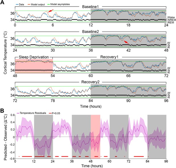
Results of Model 0 with constant asymptotes.
(A) A representative example of a 96-hr recording in one mouse of brain temperature (blue) and simulated data (orange). Green lines represent the model's lower and upper asymptotes. The 4-s hypnogram of wake (W), non–rapid-eye-movement sleep (N), and rapid-eye-movement sleep (R) appears above the lower asymptote. White/gray backgrounds represent 12 hr light–dark periods, respectively, and the salmon background starting at 48 hr indicates the 6 hr of sleep deprivation. Red arrows point to examples of over/under estimation of the model in the light–dark periods, respectively. (B) Hourly differences (mean ± STD) between simulation output and data. Red marks below the graph represent significant differences, tested by paired t-tests and false discovery rates corrected at p<0.05. Hourly values are plotted at the interval midpoint. White/gray/salmon backgrounds as in (A).
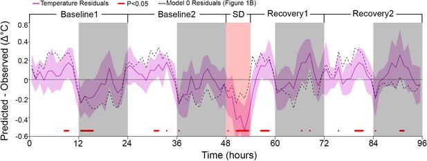
Residuals of the model in which both asymptotes were modulated according to a circadian rhythm.
Residuals (as in Figure 1B) of the basic model after adding a circadian element by modulating both asymptotes according to a sine-wave function with amplitude and phase as free parameters (the period was set to 24 hr). Note the ~0.5°C underestimation during sleep deprivation (SD). Median residual RMS over all mice and hours amounted to 0.32°C. White/gray/salmon backgrounds in both panels indicate light/dark/SD periods, respectively. Dashed lines mark the mean temperature residuals of Model 0, from Figure 1B.
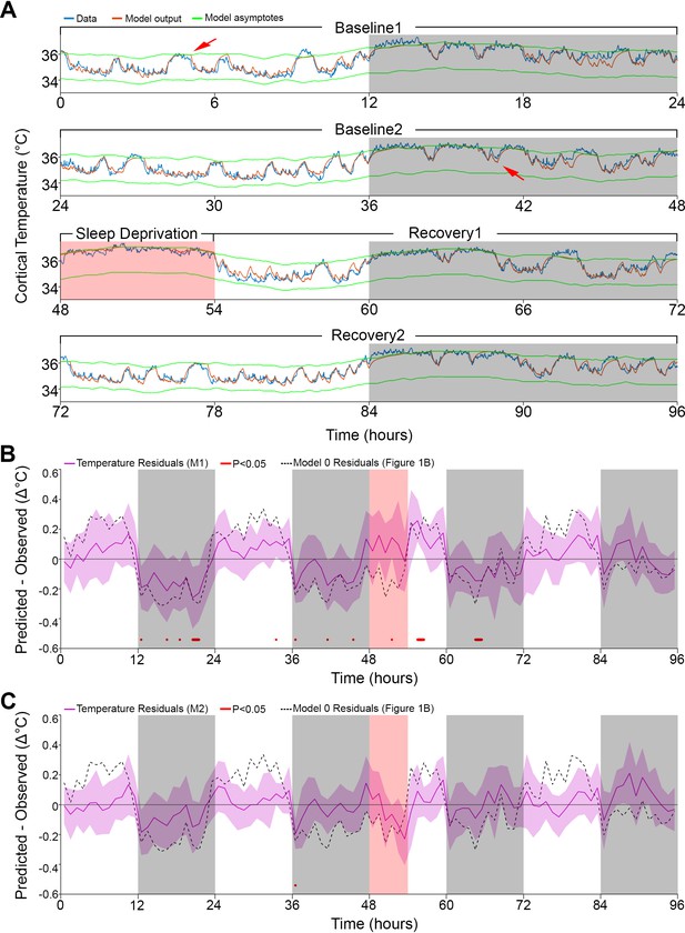
Results of models 1 and 2 with modulation of asymptotes.
(A). Simulation fit (orange) after incorporating prior wake prevalence (Model 1). Note that both asymptotes (green) are modulated in parallel, recorded data (blue line) are of the same animal as in Figure 1, and previous over- and under-estimations marked by red arrows are diminished. White/gray/salmon backgrounds indicate light/dark/SD periods, respectively. (B,C). Residuals of models 1 and 2, as in Figure 1B, after the addition of prior wake prevalence (B, Model 1, M1) and with an additional circadian rhythm modulation of both asymptotes (C, Model 2, M2). Dashed lines mark the mean temperature residuals of Model 0, from Figure 1B. Red marks indicate significant deviations from zero. Note the reduction in the number of red marks from Figure 1B, to Figure 2B to Figure 2C.
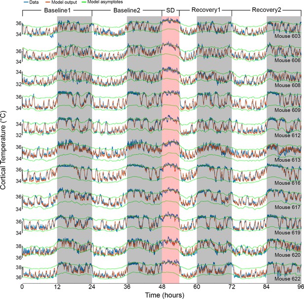
Results of Model 2 for all individual mice.
The graphs show the fit (orange) of the final model to the data (blue) of all 11 animals (ordered as in Table 1). Example data in Figures 1A and 2A correspond to mouse number 617 in the 8th row. White/gray/salmon backgrounds indicate light/dark/sleep deprivation (SD) periods, respectively.
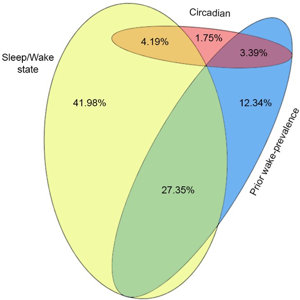
Proportional Venn diagram of the variance explained by each of the three factors in Model 2.
Yellow (41.98%), blue (12.34%), and red (1.75%) areas correspond to the unique explained variance of the sleep–wake state, prior wake-prevalence, and circadian factors, respectively. The overlapping areas in orange (4.19%), green (27.35%), and purple (3.39%) indicate the shared explained variance for any two factors. Note that the explained variance shared by all three factors was zero.
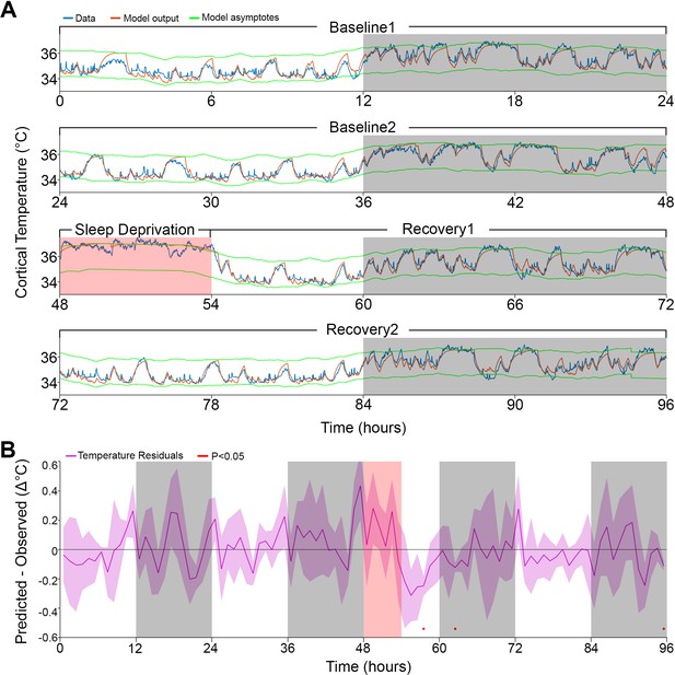
Model fit to a novel dataset.
(A) Representative example of the Model 2 fit (orange) to novel raw data (blue) not used for optimization, using the median of the optimized parameters from the original dataset (Table 1). (B) Temperature residuals of Model 2 (mean ± STD) across all animals in the novel dataset. Notice the small number of red markers, indicating significant deviations from zero. White/gray/salmon backgrounds in both panels indicate light/dark/sleep deprivation periods, respectively.
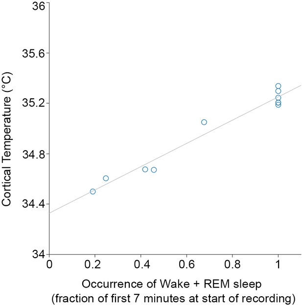
Correlation between initial temperature to wake and rapid-eye-movement (REM) sleep prevalence.
The average of the normalized temperatures (see 'Materials and methods') in the first 7 min of the recording (i.e., light onset of baseline 1) is plotted against the fraction of occurrence of wake and REM sleep in the same time window for the 11 individual recordings from the main experiment. The high correlation justifies predicting the temperature values of further sessions from sleep–wake state sequences alone.
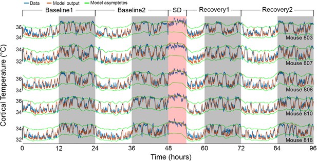
Results of Model 2 for each mouse of the independent cohort.
The graphs show the fit (orange) according to Model 2, for an additional set of five animals (data in blue), based on the median parameters of our main group of mice (Table 1). Mouse number 810 in the fourth row appears also in Figure 4A. White/gray/salmon backgrounds in both panels indicate light/dark/sleep deprivation (SD) periods, respectively.
Tables
Model 2 parameters for each animal.
Optimized values for each of the model parameters, and additional three descriptive variables: the difference between the upper and lower asymptotes (fourth column), the root mean squared error, and the correlation coefficient (two last columns). Columns 7–9 list the parameters of the prior wake-prevalence window: ‘Size’ refers to the window size, ‘Shift’ to the interval between the end of the window and the time point being evaluated, and ‘Scale’ to the conversion from % waking within the window to its temperature modulation of the asymptotes. Column 11 lists the phase of the 24-hr sinewave modulating the asymptotes (starting at zero) relative to ZT0. The last row summarizes the median value for each parameter, except for the correlation coefficient which is averaged after a Fisher transformation. Asterisks indicate KO mice.
| Animal | Asymptotes (°C) | Time constants (hr) | Prior wake prevalence | Circadian | RMS error (°C) | Correlation | ||||||
|---|---|---|---|---|---|---|---|---|---|---|---|---|
| Lower | Upper | Difference | Wake/REM | NREM | Size (hr) | Shift (hr) | Scale (°C) | Amplitude (°C) | Phase (hr) | |||
| 603 | 34.26 | 35.82 | 1.56 | 0.21 | 0.06 | 4.75 | −1.90 | 1.02 | 0.13 | 0.86 | 0.28 | 0.94 |
| 606 | 34.74 | 36.59 | 1.85 | 0.23 | 0.10 | 2.75 | −1.30 | 1.01 | 0.25 | −0.71 | 0.26 | 0.95 |
| 608 | 32.28 | 33.77 | 1.49 | 0.22 | 0.08 | 2.75 | −1.40 | 0.92 | 0.25 | −0.41 | 0.23 | 0.95 |
| 609 | 34.04 | 36.28 | 2.24 | 0.22 | 0.11 | 1.75 | −1.10 | 0.68 | 0.19 | −2.66 | 0.25 | 0.97 |
| 612 | 32.60 | 34.45 | 1.85 | 0.23 | 0.11 | 1.50 | −0.90 | 0.73 | 0.18 | −0.63 | 0.24 | 0.97 |
| 613 | 34.15 | 36.07 | 1.92 | 0.11 | 0.17 | 3.25 | −1.00 | 1.12 | 0.26 | −0.83 | 0.30 | 0.93 |
| 616* | 34.01 | 36.11 | 2.10 | 0.17 | 0.14 | 5.50 | −2.70 | 1.05 | 0.11 | 9.59 | 0.26 | 0.97 |
| 617* | 34.54 | 36.30 | 1.76 | 0.16 | 0.16 | 3.25 | −1.00 | 1.01 | 0.17 | −1.17 | 0.23 | 0.96 |
| 619* | 34.53 | 36.40 | 1.87 | 0.21 | 0.11 | 3.00 | −1.60 | 0.62 | 0.06 | −1.07 | 0.25 | 0.96 |
| 620* | 36.89 | 38.21 | 1.32 | 0.12 | 0.05 | 2.75 | −1.40 | 1.16 | 0.22 | 1.29 | 0.29 | 0.95 |
| 622 | 36.14 | 38.11 | 1.97 | 0.20 | 0.09 | 4.75 | −2.00 | 1.02 | 0.19 | −0.41 | 0.31 | 0.95 |
| Median | 34.26 | 36.28 | 1.85 | 0.21 | 0.11 | 3.00 | −1.40 | 1.01 | 0.19 | −0.63 | 0.26 | 0.96 |
Additional files
-
Source code 1
A Matlab code for the brain temperature simulation based on sleep scoring data.
- https://cdn.elifesciences.org/articles/62073/elife-62073-code1-v1.zip
-
Source code 2
A Matlab code for optimization of the parameters needed for simulation of brain temperature, by minimizing the mean squared error of the difference between the model and the temperature recorded.
- https://cdn.elifesciences.org/articles/62073/elife-62073-code2-v1.zip
-
Source code 3
A Matlab code of an example for simulating brain temperature using Source Code File 1.
The code uses the data example in Source Code File 5.
- https://cdn.elifesciences.org/articles/62073/elife-62073-code3-v1.zip
-
Source code 4
A Matlab code of an example for parameters optimization using Source Code File 2.
The code uses the data example in Source Code File 5.
- https://cdn.elifesciences.org/articles/62073/elife-62073-code4-v1.zip
-
Source code 5
A Matlab file that includes example data (recorded temperature and respective sleep scoring) from one mouse, for running the example code files (Source Code Files 3 and 4).
- https://cdn.elifesciences.org/articles/62073/elife-62073-code5-v1.zip
-
Supplementary file 1
Model 0 parameters for each animal.
A table showing the optimized values for each of the four parameters of Model 0 without modulation of asymptotes, and the three additional descriptive variables, as in Table 1.
- https://cdn.elifesciences.org/articles/62073/elife-62073-supp1-v1.docx
-
Supplementary file 2
Model 1 parameters for each animal.
A table showing the optimized values for each of the parameters of the model after introducing a modulation of both asymptotes according to the prior wake-prevalence in the window preceding the assessment of temperature. Further details as in Table 1.
- https://cdn.elifesciences.org/articles/62073/elife-62073-supp2-v1.docx
-
Supplementary file 3
Performance of Model 2 for additional sleep deprivation (SD) experiments of the same animals.
The table shows the Pearson’s correlation coefficient (r) and root mean squared (RMS) error for five animals from the main experiment, after undergoing additional SD of shorter duration. Due to technical problems, the 2 hr SD experiment is missing for mouse number 622. See Table 1 for the individual optimized parameters used (asterisks denote KO mice).
- https://cdn.elifesciences.org/articles/62073/elife-62073-supp3-v1.docx
-
Supplementary file 4
An Excel file documenting the recorded and simulated data for all 11 animals of the main experiment, in 4 s resolution.
The data include the sleep scoring, the recorded temperature, and the simulated temperature for each of the three models.
- https://cdn.elifesciences.org/articles/62073/elife-62073-supp4-v1.xlsx
-
Transparent reporting form
- https://cdn.elifesciences.org/articles/62073/elife-62073-transrepform-v1.pdf


