Figures and data in Topographic gradients of intrinsic dynamics across neocortex

Figures
Additional files

6 figures and 5 additional files

Figures

Figure 1

Download asset Open asset

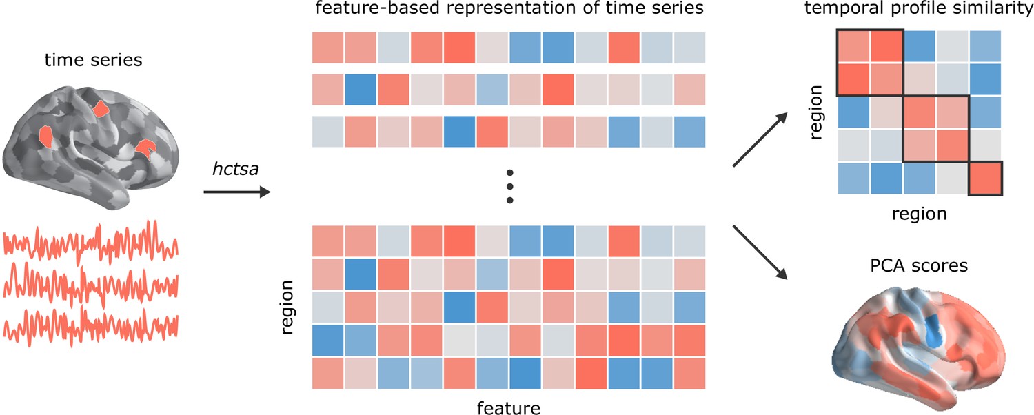
Temporal phenotyping of regional dynamics.

The highly comparative time-series analysis toolbox, *hctsa* (Fulcher et al., 2013; Fulcher and Jones, 2017), was used to extract 6441 time-series features of the parcellated time-series for each brain region and participant, including measures of autocorrelation, variance, spectral power, entropy, etc. Regional time-series profiles were then entered into two types of analyses. In the first analysis, pairs of regional time-series feature vectors were correlated to generate a region × region temporal profile similarity network. In the second analysis, principal component analysis (PCA) was performed to identify orthogonal linear combinations of time-series features that vary maximally across the cortex.

Figure 2 with 2 supplements

Download asset Open asset

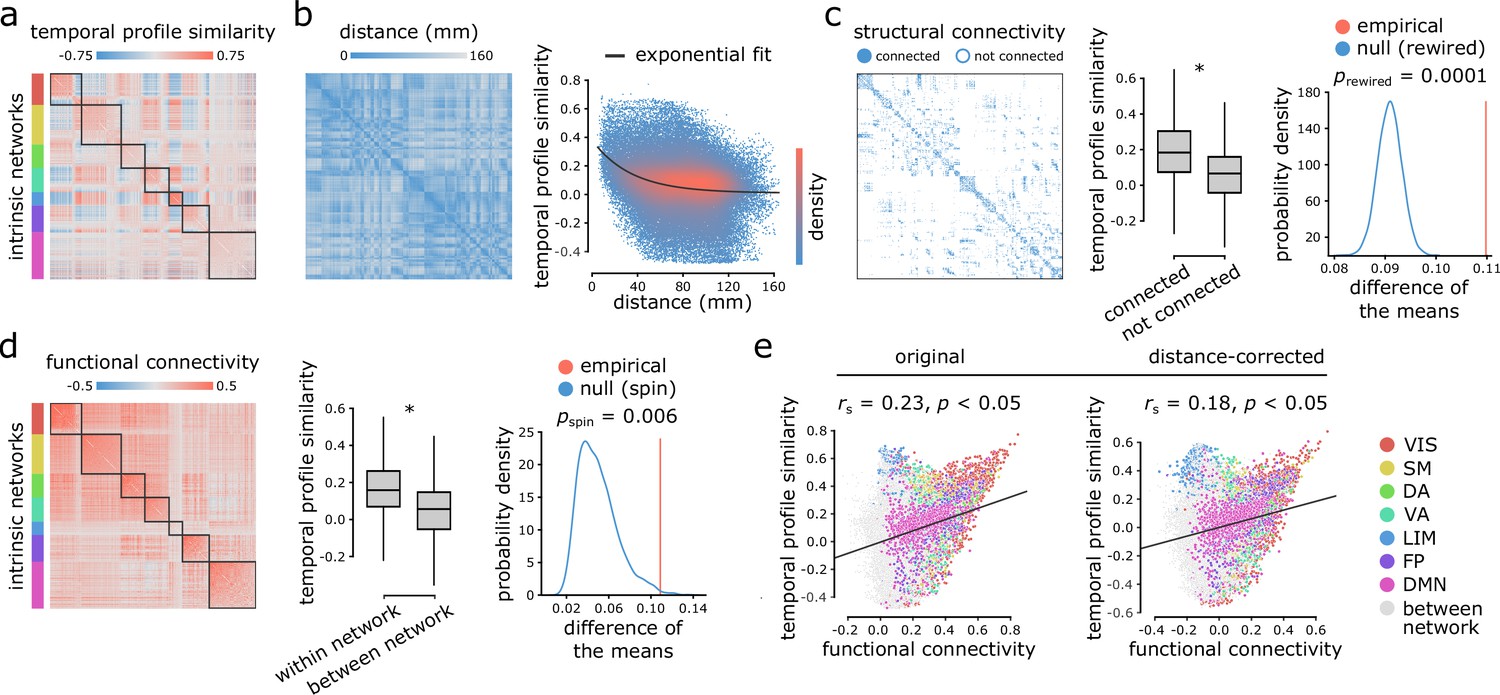
Inter-regional temporal profile similarity reflects network geometry and topology.

(a) Temporal profile similarity networks are constructed by correlating pairs of regional time-series feature vectors. Brain regions are ordered based on their intrinsic functional network assignments (Yeo et al., 2011; Schaefer et al., 2018). (b) Temporal profile similarity between regions significantly decreases as a function of Euclidean distance between them. The black line represents an exponential fit as $y = 0.37 e^{- 0.03 x} + 0.01$ , where y is temporal profile similarity and x is Euclidean distance. (**c, d**) Regional time-series features are compared between pairs of cortical areas using their structural and functional connectivity profiles. Pairwise temporal profile similarity is significantly higher among structurally-connected areas (c), and among regions that belong to the same intrinsic functional networks (d). Asterisks denote a statistically significant difference of the means (two-tailed t-test; $p \approx 0$ ). For structural networks, statistical significance of the difference of the mean temporal profile similarity of connected and unconnected node pairs is also assessed against a null distribution of differences generated from a population degree- and edge length-preserving rewired networks (Betzel and Bassett, 2018) (c, right-most panel). For functional networks, statistical significance of the difference of the mean temporal profile similarity of within and between intrinsic networks is also assessed against a null distribution of differences generated by spatial autocorrelation-preserving label permutation (‘spin tests’; Alexander-Bloch et al., 2018) (d, right-most panel). (e) Temporal profile similarity is positively correlated with functional connectivity. This relationship remains after partialling out Euclidean distance between regions from both measures using exponential trends. $r_{s}$ denotes the Spearman rank correlation coefficient; linear regression lines are added to the scatter plots for visualization purposes only. Connections are color-coded based on the intrinsic network assignments (Yeo et al., 2011; Schaefer et al., 2018). VIS = visual, SM = somatomotor, DA = dorsal attention, VA = ventral attention, LIM = limbic, FP = fronto parietal, DMN = default mode.

Figure 2—figure supplement 1

Download asset Open asset

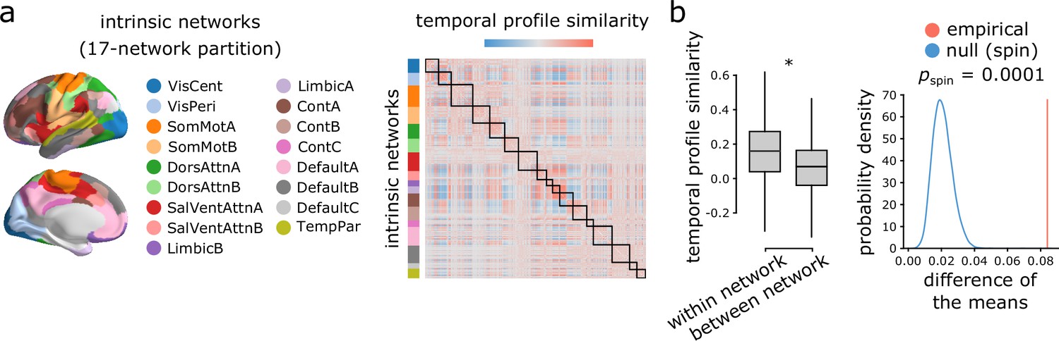
Intrinsic networks: 17 network partition.

(a) Regional time-series features are compared between pairs of cortical areas using their functional connectivity profiles. Cortical areas are ordered based on their intrinsic network assignments (17-network partition) (Yeo et al., 2011; Schaefer et al., 2018). (b) Pairwise temporal profile similarity is significantly higher among regions that belong to the same intrinsic functional networks. Asterisk denotes a statistically significant difference of the mean temporal profile similarity (two-tailed t-test; $t (79, 798) = 31.151$ ; $p \approx 0$ ). The results are consistent when the distance effect is regressed out from temporal profile similarity using the exponential trend identified in Figure 2b (two-tailed t-test; $t (79, 798) = 21.193$ ; $p \approx 0$ ). Statistical significance of the difference of the mean temporal profile similarity of within and between intrinsic networks is also assessed against a null distribution of differences generated by spatial autocorrelation-preserving label permutation (‘spin tests’; Alexander-Bloch et al., 2018) (10,000 spatial permutations; right-most panel).

Figure 2—figure supplement 2

Download asset Open asset

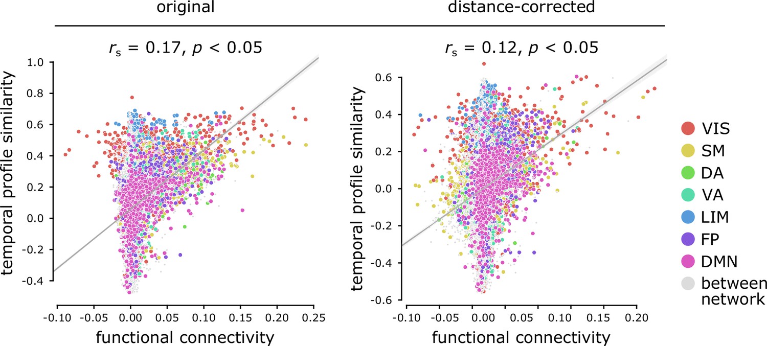
Functional connectivity measured by partial correlations.

For completeness, all functional connectivity analyses were repeated using partial correlations, as implemented in *Nilearn* (Abraham et al., 2014). Temporal profile similarity is positively correlated with functional connectivity estimated using partial correlations. This relationship remains after partialling out Euclidean distance between regions from both measures using exponential trends. $r_{s}$ denotes Spearman rank correlation coefficients; linear regression lines are added to the scatter plots for visualization purposes only. Connections are color-coded based on the intrinsic network assignments (Yeo et al., 2011; Schaefer et al., 2018). VIS = visual, SM = somatomotor, DA = dorsal attention, VA = ventral attention, LIM = limbic, FP = fronto parietal, DMN = default mode.

Figure 3 with 1 supplement

Download asset Open asset

Topographic gradients of intrinsic dynamics.

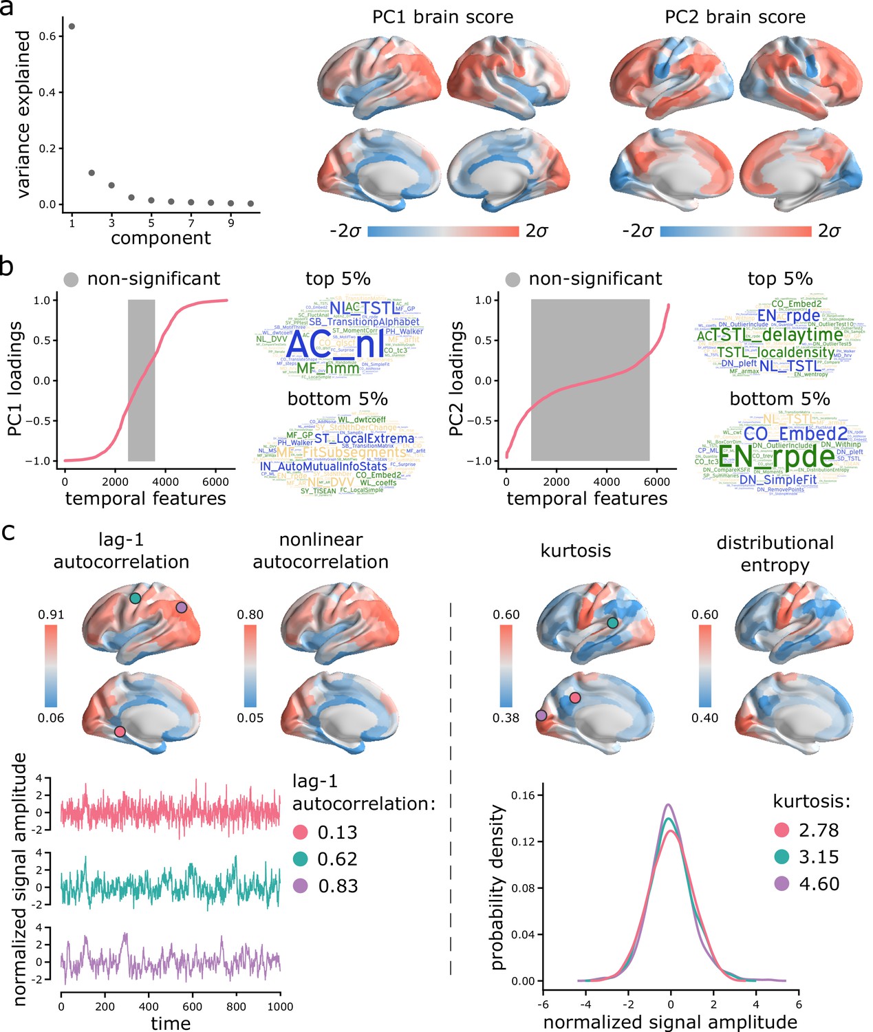
(a) PCA analysis identified linear combinations of hctsa time-series features with maximum variance across the cortex. Collectively, the first two components (PC1 and PC2) account for 75% of the total variance in time-series features of BOLD dynamics. To estimate the extent to which cortical regions display the patterns of intrinsic dynamics captured by each component, *hctsa* matrices were projected back onto the PC weights (eigenvectors), yielding spatial maps of brain scores for each component. Spatial maps are depicted based on the standard deviation $σ$ of their respective brain score distributions. (b) To understand the feature composition of the intrinsic dynamic patterns captured by PC1 and PC2, feature loadings were computed by correlating individual *hctsa* feature vectors with the PC score maps. PC loadings thus estimate the shared spatial variance between an individual time-series feature and the composite intrinsic dynamic map captured by a PC. time-series features are ordered by their individual loadings. Grey indicates non-significance based on 10,000 spatial permutation tests (FDR correction, $α = 0.001$ ). Features corresponding to the top and bottom 5% of PC1 and PC2 are visualized using word clouds. The complete list of features (ranked by loading), their definitions, correlations and p-values for both components is presented in machine-readable format in Supplementary files 3 and 4. Feature nomenclature in *hctsa* is organized such that the term prefix indicates the broad class of measures (e.g. AC = autocorrelation, DN = distribution) and the term suffix indicates the specific measure (for a complete list, see https://hctsa-users.gitbook.io/hctsa-manual/list-of-included-code-files). (c) The spatial distributions of two high-loading representative time-series features are depicted for each component, including lag-1 linear autocorrelation (AC_1) and lag-[0,2,3] nonlinear autocorrelation (AC_nl_023, estimated as average $< x_{t}^{2} x_{t - 2} x_{t - 3} >$ across time-series x) for PC1; and kurtosis (DN_Moments_4) and entropy (EN_DistributionEntropy_ks__02) of the time-series points distribution for PC2. To build intuition about what each component reflects about regional signals, three regional time-series from one participant are selected based on their lag-1 autocorrelation and kurtosis (circles on the brain surface: pink = 5th percentile, green = 50th percentile, purple = 95th percentile). Going from low-ranked to high-ranked regions results in a slowing down of BOLD fluctuations for the former and increasingly heavier symmetric tails of the signal amplitude distributions for the latter. Note that normalized feature values are shown in the first row, whereas the raw feature values are shown in the second row.

Figure 3—figure supplement 1

Download asset Open asset

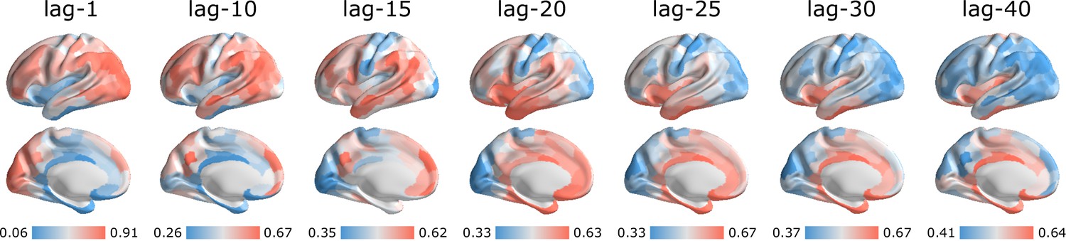
Linear autocorrelation function.

Linear autocorrelation function is depicted on the brain surface at varying time lags. The autocorrelation values are normalized between 0 and 1 using an outlier-robust sigmoidal transform and spatial maps are depicted based on the standard deviation σ of their respective distributions. Short-lag autocorrelation measures load positively on PC1, while long-lag autocorrelation measures load negatively, consistent with the notion that autocorrelation decays with increasing time lag (Figure 3).

Figure 4 with 2 supplements

Download asset Open asset

Hierarchical organization of intrinsic dynamics.

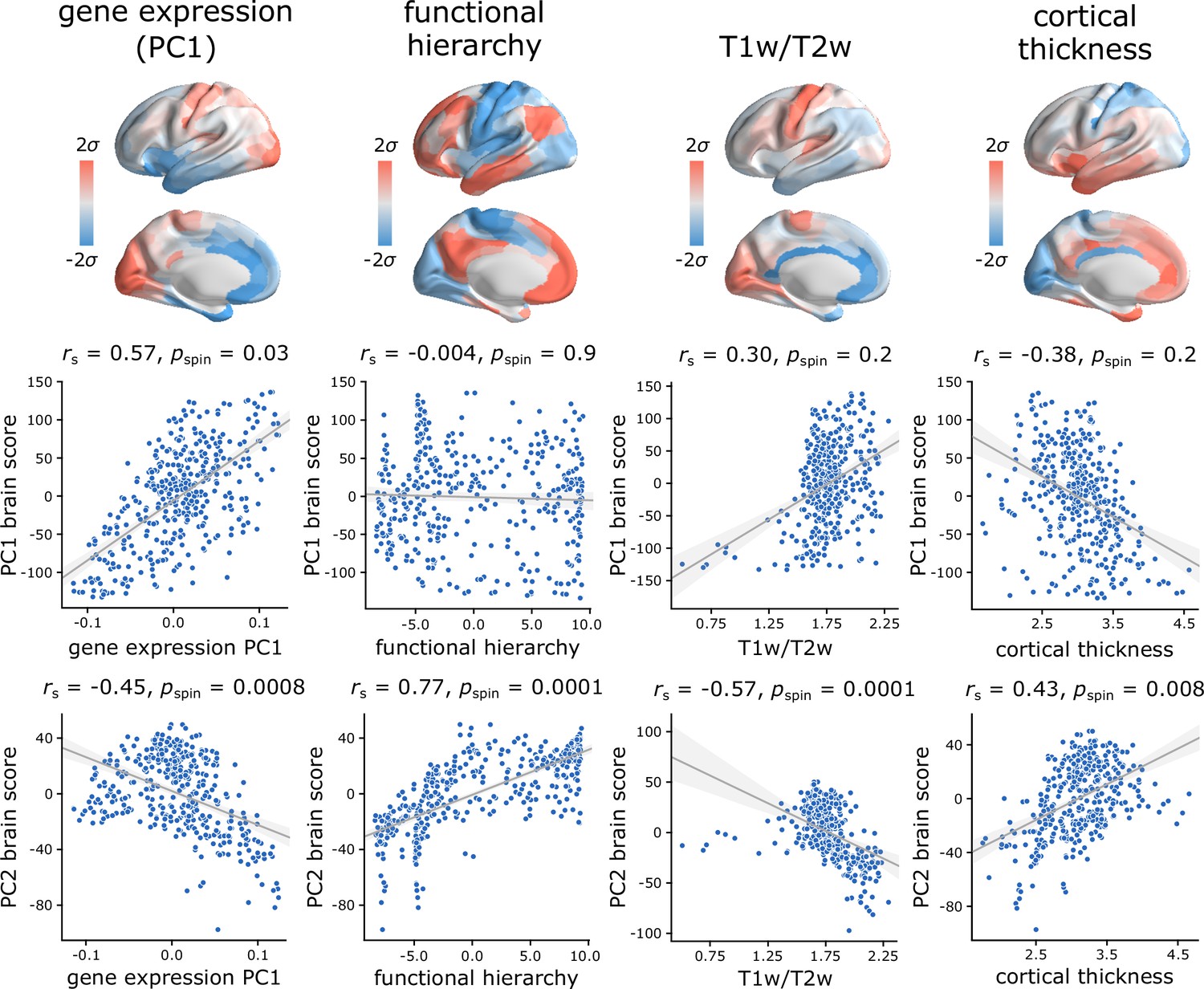
PC1 and PC2 brain score patterns are compared with four molecular, microstructural and functional maps. These maps include the first principal component of microarray gene expression data from the Allen Human Brain Atlas (Hawrylycz et al., 2012; Burt et al., 2018), the first (principal) gradient of functional connectivity estimated using diffusion map embedding (Margulies et al., 2016; Coifman et al., 2005; Langs et al., 2015), group-average T1w/T2w ratio, and group-average cortical thickness. The three latter indices were computed from the HCP dataset (Van Essen et al., 2013). Statistical significance of the reported Spearman rank correlation $r_{s}$ is assessed using 10,000 spatial permutations tests, preserving the spatial autocorrelation in the data (‘spin tests’; Alexander-Bloch et al., 2018). Linear regression lines are added to the scatter plots for visualization purposes only.

Figure 4—figure supplement 1

Download asset Open asset

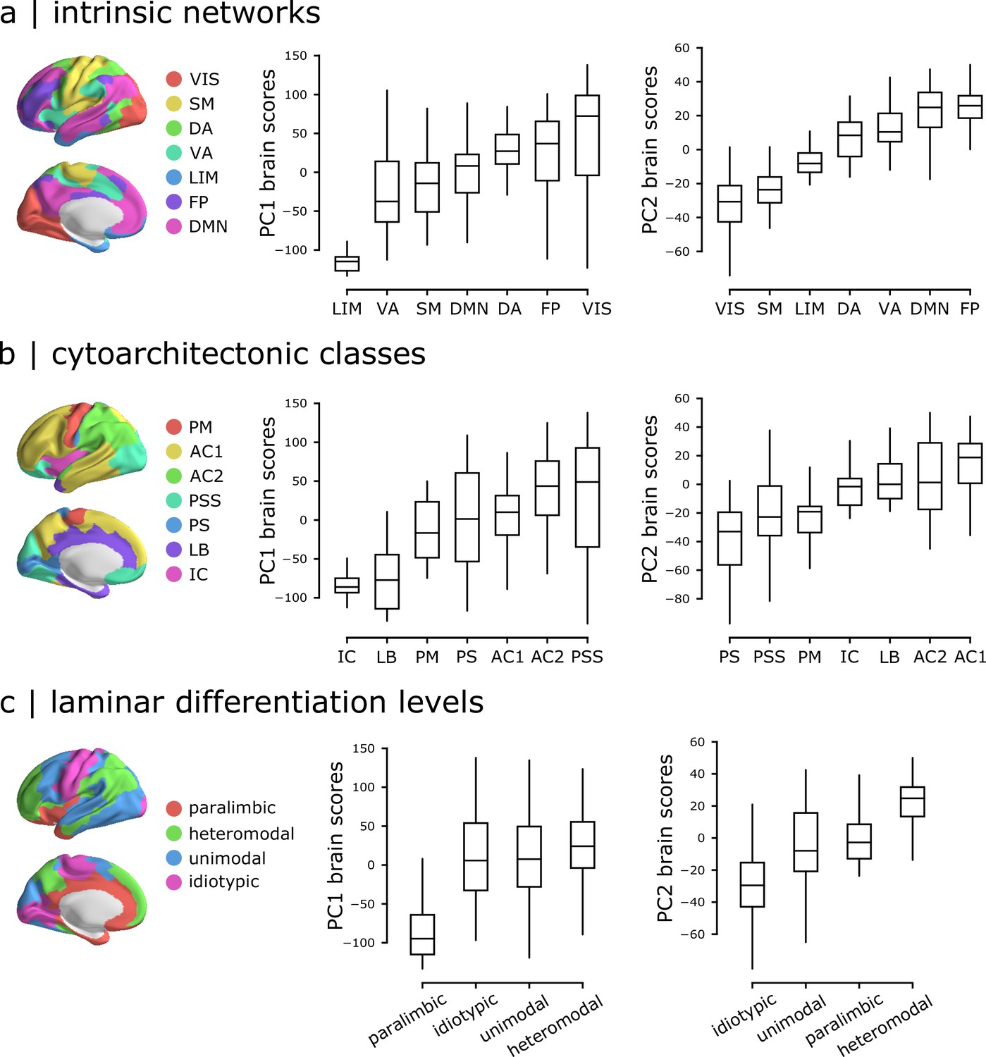
Intrinsic dynamics across intrinsic networks, cytoarchitectonic classes and laminar differentiation levels.

Mean PC1 and PC2 scores were computed for the constituent classes in three commonly used anatomical and functional partitions of the brain: (a) intrinsic fMRI networks (Yeo et al., 2011; Schaefer et al., 2018), (b) cytoarchitectonic classes (von Economo and Koskinas, 1925; von Economo et al., 2008; Vértes et al., 2016), laminar differentiation levels (Mesulam, 2000). Intrinsic networks: VIS = visual, SM = somatomotor, DA = dorsal attention, VA = ventral attention, LIM = limbic, FP = fronto parietal, DMN = default mode. Cytoarchitectonic classes: PM = primary motor cortex, AC1 = association cortex, AC2 = association cortex, PSS = primary/secondary sensory, PS = primary sensory cortex, LB = limbic regions, IC = insular cortex.

Figure 4—figure supplement 2

Download asset Open asset

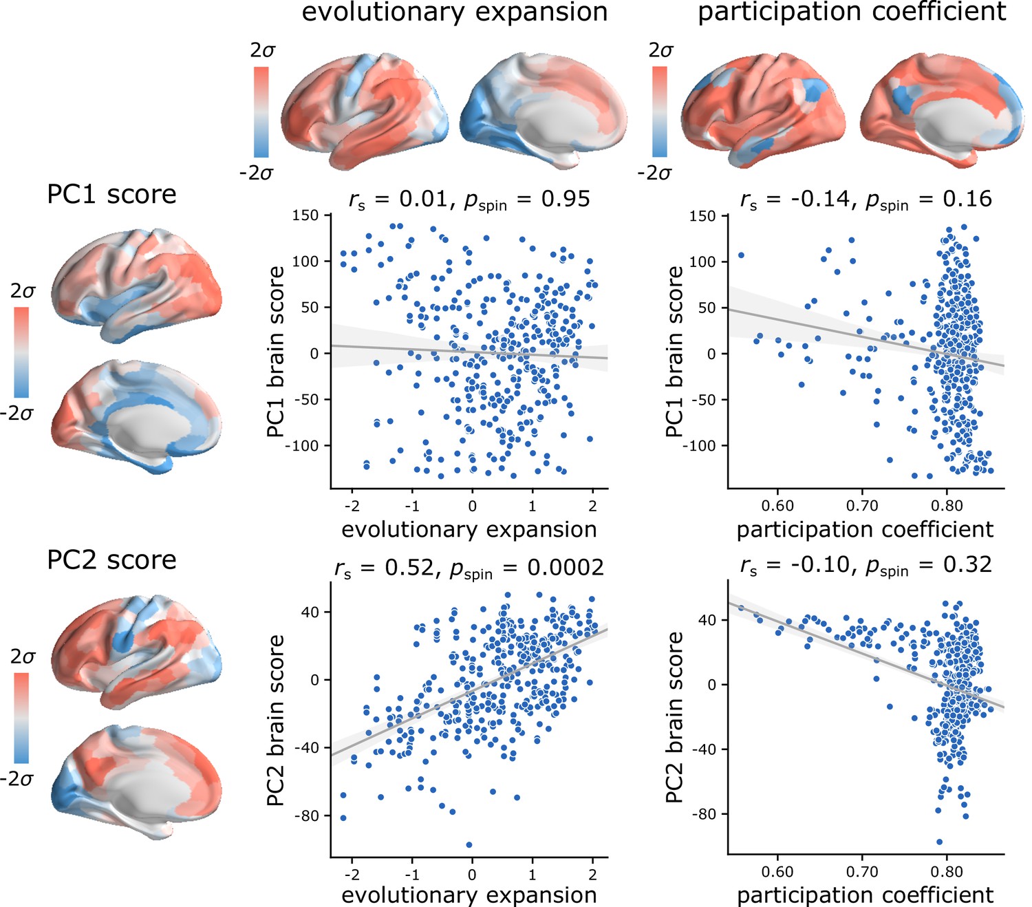
Topographic organization of intrinsic dynamics compared to evolutionary expansion and participation coefficient.

The evolutionary expansion map (Hill et al., 2010; Baum et al., 2020) was obtained through https://github.com/PennLINC/Brain_Organization and parcellated into 400 cortical areas using the Schaefer parcellation (Schaefer et al., 2018). Regional weighted participation coefficients (*Brain Connectivity Toolbox* [Rubinov and Sporns, 2010]) were estimated from functional connectivity graphs with respect to the 7-network partition of intrinsic networks (Yeo et al., 2011; Schaefer et al., 2018). We then compared the maps to the PC1 and PC2 brain score patterns. The evolutionary expansion map was significantly correlated with PC2 topography, but not PC1 topography. The regional participation coefficient map was not significantly correlated with either PC1 or PC2 topography. Statistical significance of the reported Spearman rank correlation $r_{s}$ is assessed using 10,000 spatial permutations tests, preserving the spatial autocorrelation in the data (‘spin tests’; Alexander-Bloch et al., 2018). Linear regression lines are added to the scatter plots for visualization purposes only.

Figure 5

Download asset Open asset

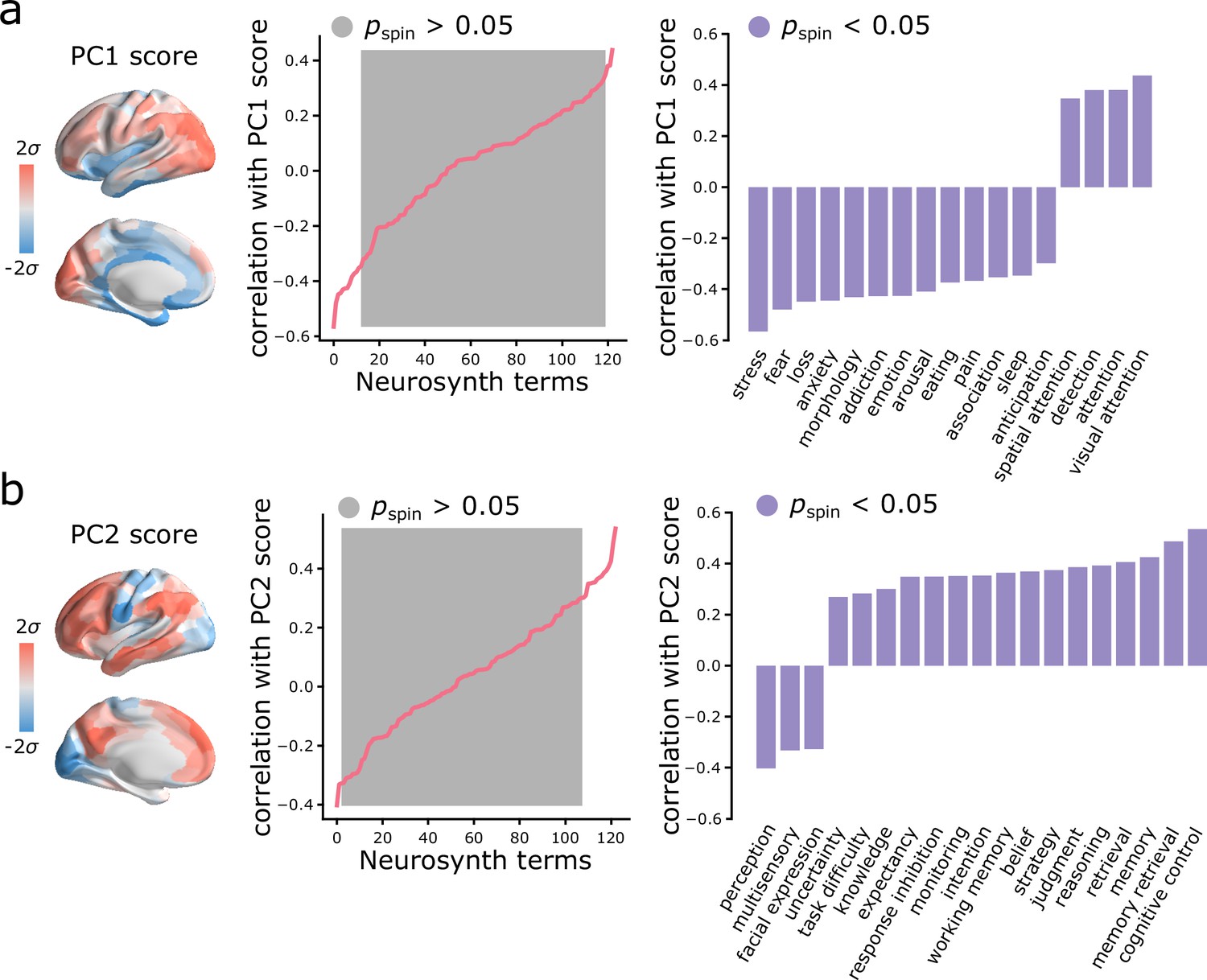
Spatial gradients of intrinsic dynamics support distinct functional activations.

We used Neurosynth to derive probability maps for multiple psychological terms (Yarkoni et al., 2011). The term set was restricted to those in the intersection of terms reported in Neurosynth and in the Cognitive Atlas (Poldrack et al., 2011), yielding a total of 123 terms (Supplementary file 2). Each term map was correlated with the PC1 (a) and PC2 (b) score maps to identify topographic distributions of psychological terms that most closely correspond to patterns of intrinsic dynamics. Grey indicates non-significance based on 10,000 spatial permutation tests (Bonferroni correction, $α = 0.05$ ). Statistically significant terms are shown on the right.

Figure 6

Download asset Open asset

Sensitivity and replication analyses.

For all comparisons, we correlated PC1 and PC2 scores and weights obtained in the original analysis and in each new analysis. Significance was assessed using spatial autocorrelation preserving nulls. Specific analyses include: (a) comparing group-level and individual subject-level results, (b) comparing data with and without grey-matter signal regression, (c) comparing functional (Schaefer) and anatomical parcellations (Desikan-Killiany), (d) comparing HCP *Discovery* and *Validation* datasets, (e) comparing HCP *Discovery* and Midnight Scan Club datasets.

Additional files

Supplementary file 1 Dominance analysis. Dominance Analysis was used to quantify the distinct contributions of inter-regional Euclidean distance, structural connectivity, and functional connectivity to temporal profile similarity (Budescu, 1993; Azen and Budescu, 2003) (https://github.com/dominance-analysis/dominance-analysis). Dominance analysis is a method for assessing the relative importance of predictors in regression or classification models. The technique estimates the relative importance of predictors by constructing all possible combinations of predictors and quantifying the relative contribution of each predictor as additional variance explained (i.e. gain in $R^{2}$ ) by adding that predictor to the models. Specifically, for p predictors we have $2^{p} - 1$ models that include all possible combinations of predictors. The incremental $R^{2}$ contribution of each predictor to a given subset model of all the other predictors is then calculated as the increase in $R^{2}$ due to the addition of that predictor to the regression model. Here we first constructed a multiple linear regression model with distance, structural connectivity and functional connectivity as independent variables and temporal profile similarity as the dependent variable to quantify the distinct contribution of each factor using dominance analysis. The total $R^{2}$ is 0.28 for the complete model that includes all variables. The relative importance of each factor is summarized in the table, where each column corresponds to: Interactional Dominance is the incremental $R^{2}$ contribution of the predictor to the complete model. For each variable, interactional dominance is measured as the difference between the $R^{2}$ of the complete model and the $R^{2}$ of the model with all other variables except that variable; Individual Dominance of a predictor is the $R^{2}$ of the model when only that predictor is included as the independent variable in the regression; Average Partial Dominance is the average incremental $R^{2}$ contributions of a given predictor to all possible subset of models except the complete model and the model that only includes that variable; Total Dominance is a summary measure that quantifies the additional contribution of each predictor to all subset models by averaging all the above measures for that predictor; Percentage Relative Importance is the percent value of the Total Dominance.: https://cdn.elifesciences.org/articles/62116/elife-62116-supp1-v2.docx
Download elife-62116-supp1-v2.docx
Supplementary file 2 List of terms used in Neurosynth analyses. The overlapping terms between Neurosynth (Yarkoni et al., 2011) and Cognitive Atlas (Poldrack et al., 2011) corpuses used in the reported analyses are listed below.: https://cdn.elifesciences.org/articles/62116/elife-62116-supp2-v2.docx
Download elife-62116-supp2-v2.docx
Supplementary file 3 List of time-series features corresponding to PC1. The complete list of features (ranked by loading), their definitions, correlations and p-values for PC1 is presented in machine-readable format.: https://cdn.elifesciences.org/articles/62116/elife-62116-supp3-v2.xls
Download elife-62116-supp3-v2.xls
Supplementary file 4 List of time-series features corresponding to PC2. The complete list of features (ranked by loading), their definitions, correlations and p-values for PC2 is presented in machine-readable format.: https://cdn.elifesciences.org/articles/62116/elife-62116-supp4-v2.xls
Download elife-62116-supp4-v2.xls
Transparent reporting form: https://cdn.elifesciences.org/articles/62116/elife-62116-transrepform-v2.docx
Download elife-62116-transrepform-v2.docx