Performance in even a simple perceptual task depends on mouse secondary visual areas
- Unit on Neural Computation and Behavior, National Institute of Mental Health Intramural Program, National Institutes of Health, United States
Figures
Figure 1 with 4 supplements
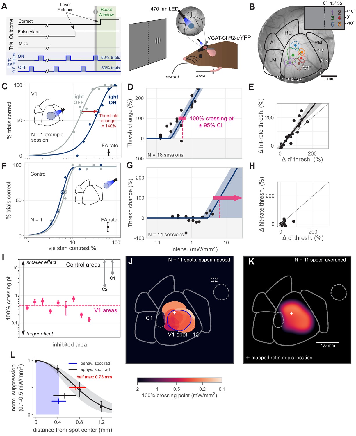
Optogenetic inhibition of V1 confirmed to affect behavior.
(A) Schematic of the visual detection behavior task. Animals release a lever when they detect the onset of a visual stimulus. Stimuli were Gabor patches of varying contrast presented on a neutral gray screen. Cortical activity was suppressed via optogenetic activation of inhibitory neurons (VGAT-ChR2-EYFP mouse line). On each trial, a train of light pulses was applied to the cortex (Materials and methods). Visual stimuli were delivered either during a light pulse (light ON trials) or when the light pulse was off (light OFF trials). (B) Cortical areas were identified using hemodynamic intrinsic imaging of cortical responses to a set of visual stimuli at different positions within visual space (Materials and methods, Figure 1—figure supplement 1). (C) LED stimulation in V1 decreases performance (single session; light intensity = 0.46 mW/mm2; rightward shift indicates decreased performance). Filled circles: performance at one contrast. Open circles: threshold (63% point of fit curve). False alarm (FA) rate is estimated FA hazard rate (Materials and methods). Lower asymptote of psychometric function is fixed at zero. Upper asymptote (lapse rate) is allowed to vary. (D) Piecewise-linear function fit to all sessions from the spot in panel C, measuring the intensity required to double the psychometric threshold (N = 18 sessions, 100% crossing point, pink; mean 0.57, bootstrap 95% CI 0.43–0.71 mW/mm2). Slopes were fit by pooling across stimulation locations and experimental sessions; fitting slope separately for each session produced similar results (Figure 1—figure supplement 3). (E) Change in d′ threshold increase vs change in hit-rate threshold increase, for the spot in panel C. (F) Single session example behavior from LED stimulation in a control area outside of V1 (light intensity = 1.3 mW/mm2), same conventions as panel C. (G) Same as D, fit to sessions from control spot in panel F (N = 14 sessions, mean 100% crossing point 6.6, bootstrap 95% CI 4.3–7.6 mW/mm2). (H) Same as panel E, fit to sessions from the control spot in panel F. (I) 100% crossing points for all V1 spots and two control spots, as determined by regression fits in E and G. Ordering of spots is arbitrary; points are offset along x axis to allow display of confidence intervals for each point. (J) Contours of all V1 spots and controls, color weighted by 100% crossing point. Spot contours are the full width at half-max of the Gaussian light distribution produced by the fibers (N = 11 spots, Figure 1—figure supplement 2). (K) Heatmap of effect size in V1, generated by averaging the 100% crossing point for each spot at each pixel (N = 11 spots). (L) Spatial fall-off of inhibition. Y-axis: suppression of visual responses measured with electrophysiology (silicon probe, four shanks), light intensity between 0.1 and 0.5 mW/mm2 (N = 4 experiments, black line: Gaussian fit, gray: 95% CI via bootstrap; data error bars: SEM, N = 45 single units). Full width at half max of Gaussian fit = 0.73 mm, bootstrap 95% CI 0.61–0.92 (red line). Electrophysiology spot radius: 0.53 ± 0.21 mm (black line, mean ± SD). Behavioral spot radius: 0.42 ± 0.13 mm (blue shaded area and line, mean ± SD, N = 34 inhibitory light spots). Since behavioral spots are smaller on average than what was used for these physiology experiments, the spatial effect of inhibition during behavior is likely more restricted than shown by these suppression data (black curve, red bar).
Figure 1—figure supplement 1
Visual area identification via imaging.
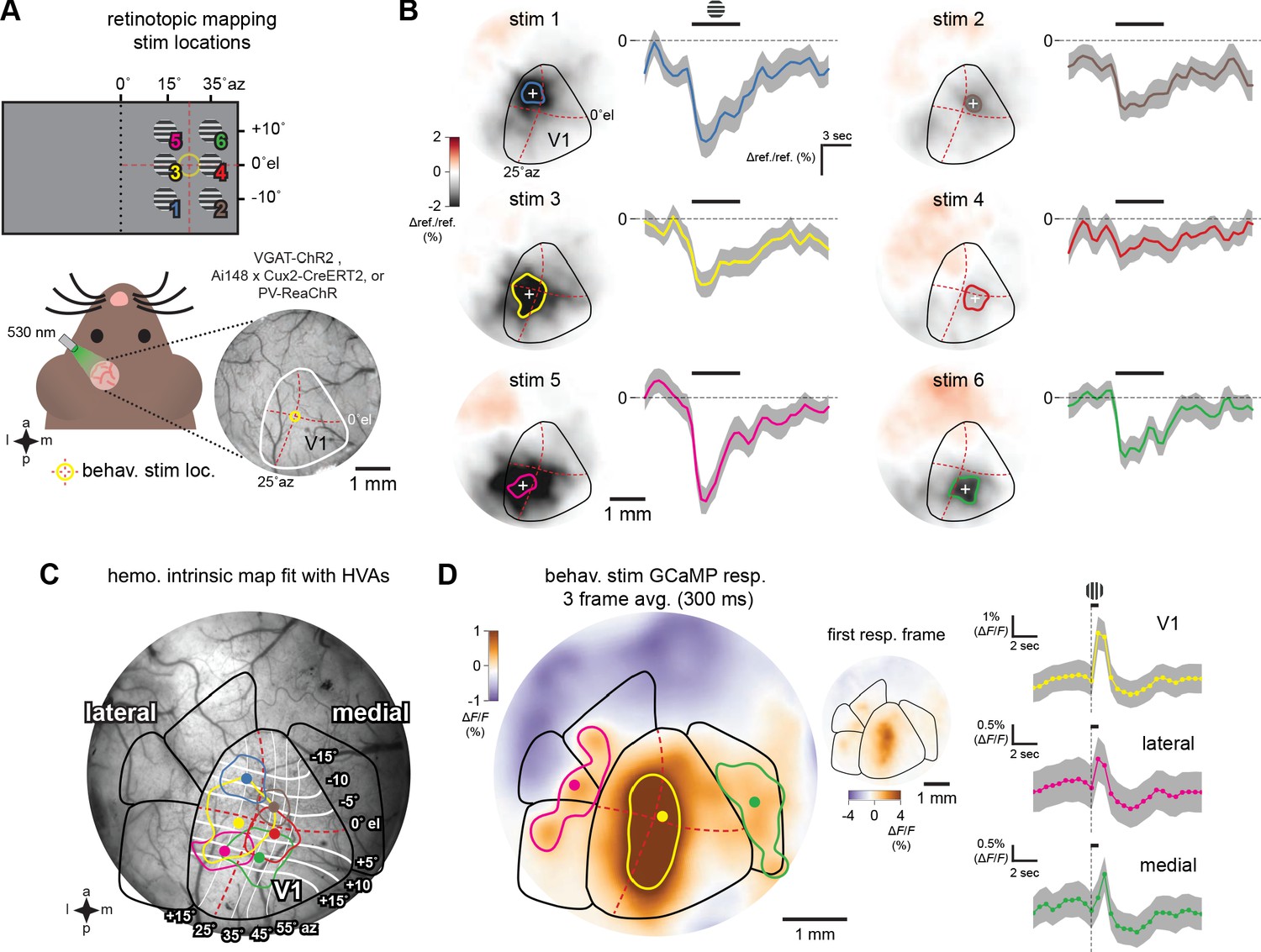
Intrinsic hemodynamic and GCaMP imaging to fit and test visual area maps. (A) Schematic of hemodynamic intrinsic imaging. Gabor stimuli with upward drifting gratings were presented to head-fixed animals randomly at six locations in their right visual field (Materials and methods). Each stimulus was shown to the animal 30 times. The cortical surface was evenly illuminated using a fiber coupled 530 nm LED and imaged at 2 Hz through a bandpass green emission filter. Behavioral visual stimulus location is shown at the center of the hemodynamic map (yellow circle at 25° azimuth (az), 0° elevation (el), red dotted lines). (B) Averaged response map and time course of cortical reflectance change at all six stimulus locations. Increased cortical blood flow due to the visual stimulus results in a drop in reflectance (Δ ref./ref.). The period of maximal change in Δ ref./ref. (%) occurs 2 s after stimulus presentation (Heimel et al., 2007). Colored dot and boundary indicate the centroid and 50% contour. (C) Scaled and rotated retinotopic map of mouse V1 and secondary visual areas positioned using the six hemodynamic response locations in an Ai148; Cux2-CreERT2 animal which expresses GCaMP6f in L2/3 cortical excitatory neurons. Elevation and azimuth contours from Zhuang et al., 2017. (D) GCaMP6f response, averaged over three frames, to the visual stimulus used in the behavioral task (a Gabor) presented for 100 ms with 5 s of 50% gray screen between presentations. GCaMP6f fluorescence increases (ΔF/F) are prominent and well-described by the area map fit to the hemodynamic responses in V1. Colored dot and boundary indicate the centroid and 50% contour. Inset shows single-frame GCaMP6f response. Right, time courses of GCaMP6f responses. PM response latency is noticeably longer compared to either V1 or the lateral areas, consistent with electrophysiology results (Figure 6—figure supplement 1).
Figure 1—figure supplement 2
Light spot size calculations.
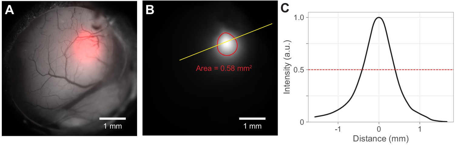
Spot size and contour were calculated from the light spot image on the cortex. (A) Example of fiber-coupled LED output from 400 µm diameter flat-faced fiber cemented over the cranial window (Materials and methods). Light spots (red) were measured by imaging with a camera the light cast by the fiber onto the cortical surface. Light emerging from fibers has a radial profile that is approximately a 2-d Gaussian. (B) To calculate spot size, light spot intensity images (the red channel from A) were filtered with a 2-d Gaussian (result: white image). (While this is the same intensity data as in the red channel that is superimposed on the gray scale window image in A, the details of the intensity distribution are more visible here). Red: 50% intensity contour. The full width at half-max was calculated as the radius of a disk with the same area as enclosed by the 50% contour (here area is 0.58 mm2; corresponding FWHM/diameter is 0.86 mm). This area was used to calculate intensity for optogenetic experiments. The filled version of this contour is used to construct heatmaps (e.g. Figure 3E). (C) Normalized intensity along the yellow line in panel B. The intensity distribution is roughly Gaussian.
Figure 1—figure supplement 3
Slope determination for piecewise-linear function.
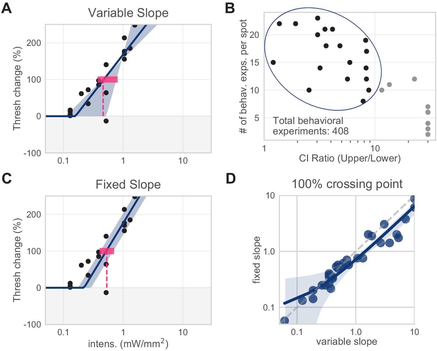
Slopes for piecewise-linear functions were determined via least-squares regression. All spots from all areas were first fit with a variable-slope piecewise-linear function. We averaged the variable slopes of spots with low slope CI ratios to determine the fixed slope used across all spots from all areas to determine 100% crossing points (295.9% threshold change/mW/mm2). (A) Example spot with variable slope fit (N = 18 sessions, mean 100% crossing pt. 0.46, bootstrap 95% CI 0.38–0.81 mW/mm2). (B) Slopes of all spots with low slope CIs. (C) Same example spot as (A), with fixed slope (N = 18 sessions, mean 100% crossing pt. 0.53, bootstrap 95% CI 0.43–0.71 mW/mm2). (D) Fixing the slope did not dramatically affect the 100% crossing points. Spots included here are from all visual areas.
Figure 1—figure supplement 4
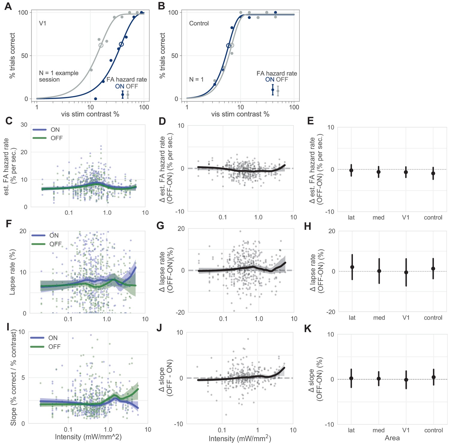
Lapse rate, estimated false alarm (FA) hazard rate, and psychometric function slope vary little with stimulation.
(A and B) Same V1 (A) and control (B) inhibition example session as in Figure 1C,F, here with estimated FA hazard rates plotted separately for each trial type (dark blue = ON trials, gray = OFF trials), showing the FA rates are not different between ON and OFF trials. (Estimated FA hazard rates are total FA rates, or number of trials ending in a false alarm over all trials, divided by average trial length, Materials and methods). (C–E) FA hazard rates are similar with and without optogenetic stimulation. (C) Estimated FA hazard rate (Materials and methods) plotted for each trial type, across intensity (blue = ON, green = OFF; thick line = LOWESS fit, shaded regions = 95% CI via bootstrap). The FA hazard rate does not vary with trial type even though the FA hazard rate changes slightly on light pulses (Figure 2C), likely because the light pulse train has randomized phase across trials. (D) Difference in estimated FA hazard rate across intensity (black, OFF–ON difference within each session, other conventions as in C). (E) Mean difference in estimated FA hazard rate, by inhibited area (error bars = mean ± SD). One pairwise comparison between areas yielded a weak but statistically significant difference: lateral v. control (N = 386 total sessions; Mann–Whitney U; lateral vs control: U = 1773, p = 0.048; all other pairwise comparisons were nonsignificant, U > 1819, p > 0.068, Bonferroni corrected for N = 6 comparisons). (F–H) Same as C–E, but for lapse rate. Little change was seen in lapse rate with stimulation, for differences as a function of intensity, or for differences as a function of area. While the heavy lines in F slightly exit the CI bounds at a moderate intensity, this is unlikely to be a reliable effect, considering that the line spanning different intensities creates multiple comparisons. All pairwise area comparisons nonsignificant; Mann–Whitney U; all comparisons: U > 1839, p > 0.18, Bonferroni corrected. (I–K) Same as C–E but for psychometric function slope (Weibull fit slope) for each trial type. Slope does not vary significantly by area (Mann–Whitney U; U > 1321, p > 0.36).
Figure 2
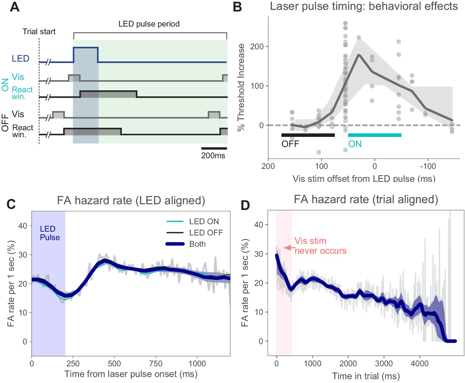
Timing of stimulus relative to pulses and false alarm rates.
(A) Timing of task events within LED pulse period. LED pulse trains were the same on each trial except the onset phase was randomized (uniform distribution, Materials and methods). Light pulse duration 200 ms (dark blue shaded region). Off duration 1000 ms (green shaded region), therefore, pulse period is 1200 ms. Pulse onset timing was chosen based on measured effects on perceptual behavior with ON pulses (panel B). Trials could last for several pulse periods. (B) Threshold increase (%) across visual stimulus offsets. Points indicate changes in perceptual threshold in individual experiments where timing offset between stimulus onset and LED pulse onset was fixed (N = 112 sessions from N = 5 animals). Solid line: LOWESS fit. (C) False alarm hazard function (probability of false alarm given the trial has lasted until that time; calculated over N = 50,382 trials that resulted in false alarms, pooled across animals and light intensities). Since stimulus onset times are randomized in this task, the false alarm hazard function is the measure that parallels hit rates for signal detection theory-based analysis (Macmillan and Creelman, 2004). Here false alarm hazard rates are plotted relative to LED pulse onset time (which is randomized relative to trial onset time). Thin gray line: false alarm hazard computed in 1 ms bins (all hazard rates are normalized to units of false alarm rate per 1 s interval: y-axis). Thick blue line: LOWESS fit. Shaded region (mostly hidden): 95% CI via bootstrap. Thin lines (also largely hidden): false alarm hazard for ON and OFF trials, showing ON and OFF trial types have similar false alarm hazard rates. (D) False alarm hazard function plotted relative to trial start time (same trials as C). Visual stimulus onset time and LED pulse onset time are both randomized relative to trial start in each trial (Materials and methods). While each trial begins with a tone at time 0, the visual stimulus onset never occurs in the first 400 ms; the initial increase in false alarm rates likely reflects subjects’ slight failure to inhibit responses to trial start. For longer times, fewer trials are in the data set and estimates become more variable. Error bars: 95% CI via bootstrap.
Figure 3 with 1 supplement
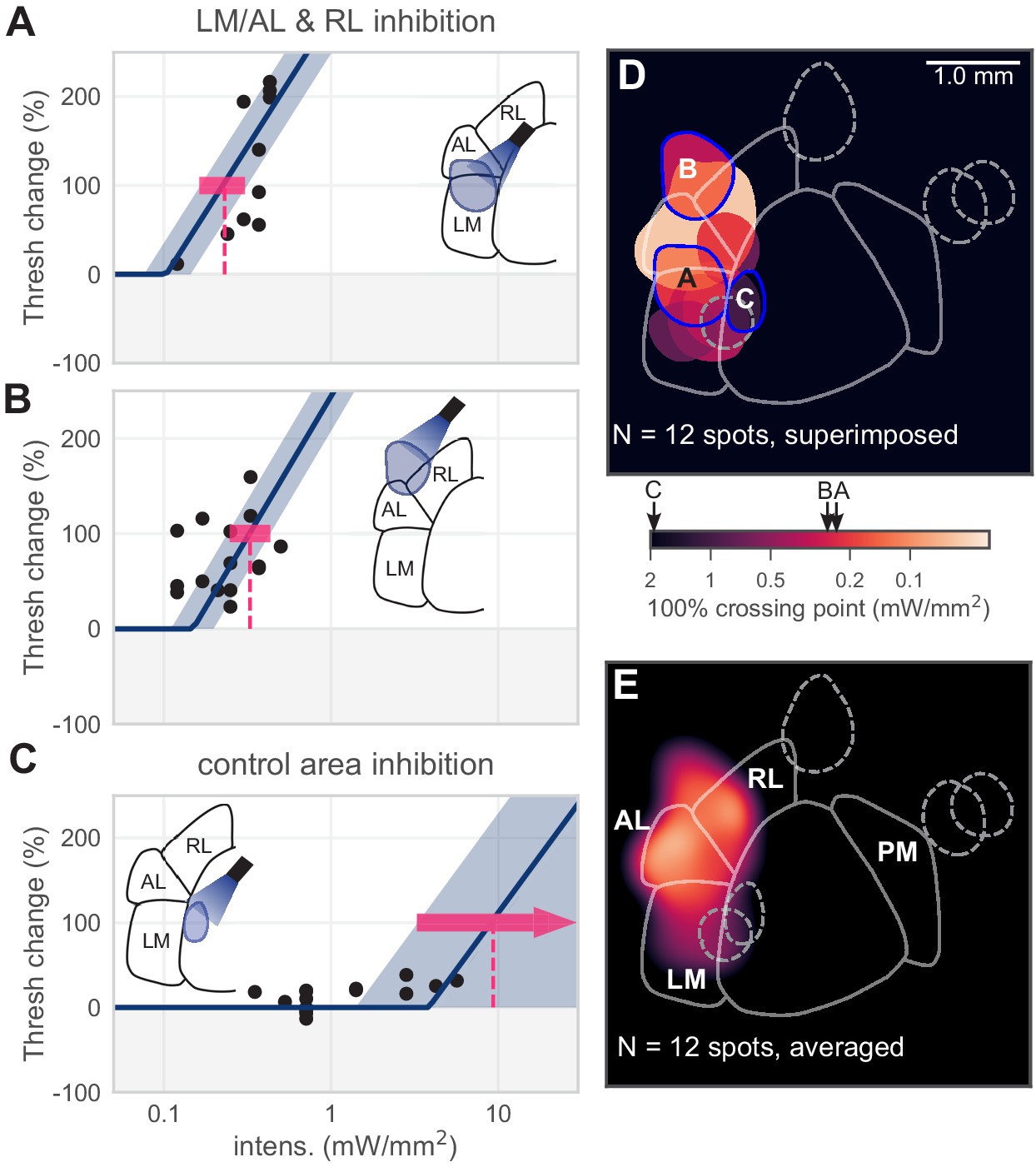
Inhibiting lateral areas degrades contrast-change detection behavior.
(A) All sessions from an example spot on the border of AL and LM, showing a large effect (N = 12 sessions, mean 100% crossing pt. 0.23, bootstrap 95% CI 0.16–0.31 mW/mm2). (B) All sessions from an example spot within RL, showing a large effect (N = 18 sessions, mean 100% crossing pt. 0.33, bootstrap 95% CI 0.25–0.43 mW/mm2). (C) All sessions from a control area between LM and V1, showing no effect even at high intensities (N = 15 sessions, mean 100% crossing pt. 8.7, bootstrap 95% CI 4.6–9.3 mW/mm2). (D) Map of spots within LM/AL/RL and control locations, colored by 100% crossing pt. Crossing points from panels A–C are shown on color bar (black arrows). (Note slight difference for visual display in color bar extents compared to Figure 1J,K). (E) Heatmap of effect size, generated by averaging the 100% crossing point at each pixel; pixels with no data are colored black.
Figure 3—figure supplement 1
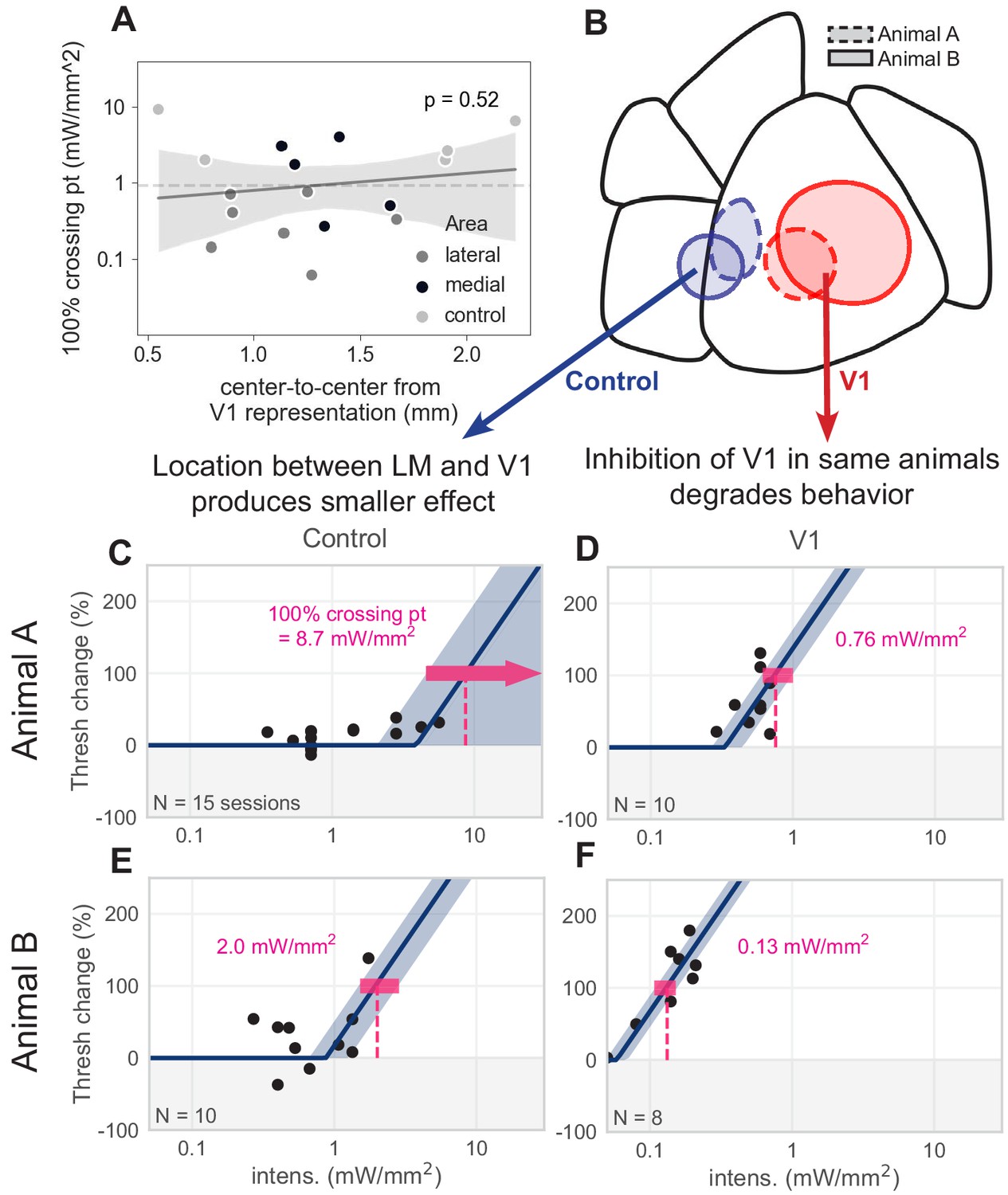
Control spots between V1 and LM.
Effects seen in LM/AL and RL are not explained by distance from V1. (A) Distance between the V1 representation of the stimulus and each spot outside V1 does not predict behavioral effect magnitude. There is no significant relationship between 100% crossing point (i.e., magnitude of effect on perceptual behavior; smaller crossing point is a larger effect on behavior) and proximity to the V1 representation (linear regression, slope not significantly different than zero,, t = 0.66, p = 0.52. Dashed line denotes mean distance from V1 representation, 0.92 mm). (B–F) We placed control spots between LM and V1 in two animals and compared effect sizes to spots placed in V1. In both cases, there was a 10-fold decrease in effect when the light spot was moved from V1 to an area between LM and V1, despite being in close proximity to both the V1 and LM retinotopic representations. (B) Schematic showing two pairs of control spots (blue) between V1 and LM, and two spots within V1 (red); each pair from a separate animal (dashed lines = Animal A, solid lines = Animal B). (C) Piecewise-linear function and 100% crossing point calculation from the control spot between LM and V1 of Animal A (100% crossing pt. = 8.7 mW/mm2, N = 15 sessions). (D) Same as C, for a spot within V1 of Animal A (100% crossing pt. = 0.76 mW/mm2, N = 10 sessions). More than a 10-fold increase in 100% crossing point exists between the effect seen in V1 and the effect seen in the control area. Note that a smaller crossing point is a larger effect of optogenetic inhibition on perceptual threshold. (E) Same, for the control spot between LM and V1 of Animal B (100% crossing pt. = 2.0 mW/mm2, N = 10 sessions). (F) Same, for the spot within V1 of Animal B (100% crossing pt. = 0.13 mW/mm2, N = 8 sessions). More than a 10-fold increase in 100% crossing point exists between the effect seen in V1 and the effect seen in the control area. (The spot shown here produces an effect ≈ 4× larger than the spot in D; this might be explained by larger spot size, or different position on the V1 retinotopic map, or both). Despite these two control spots being very near to the V1 spots, they produce much smaller effects (larger 100% crossing points). In contrast, light spots fully in LM/AL or RL (Figure 3) produce effects comparable to those seen in V1 (Figure 5).
Figure 4 with 1 supplement
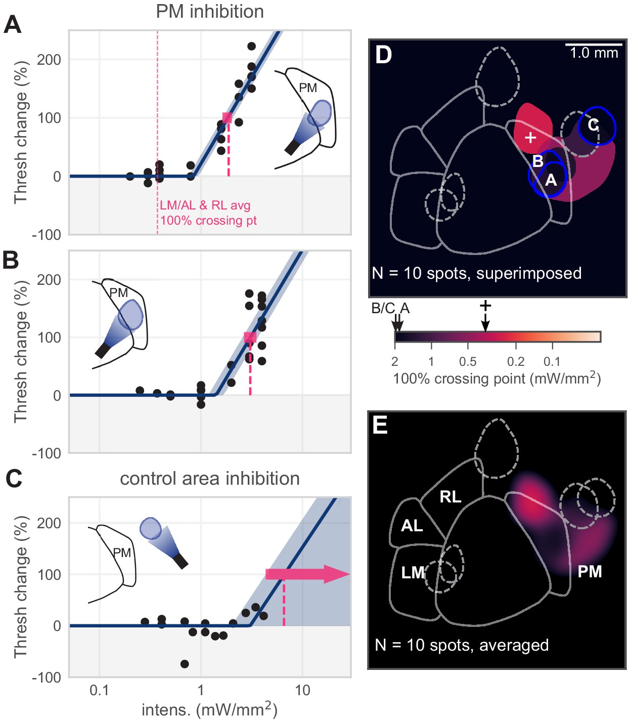
Inhibiting medial areas produces weaker effects on behavior.
(A) All sessions from an example spot within PM, which produced a weak effect (N = 22 sessions, mean 100% crossing pt. 1.9, bootstrap 95% CI 1.6–2.0 mW/mm2). Vertical pink dashed line represents average crossing point from LM/AL and RL (0.37 mW/mm2). (B) All sessions from a second example spot within PM, which also produced a weak effect (N = 23 sessions, mean 100% crossing pt. 3.1, bootstrap 95% CI 2.7–3.5 mW/mm2). (C) All sessions from a control area outside PM, showing very little effect even at high intensities (N = 14 sessions, mean 100% crossing pt. 6.6, bootstrap 95% CI 4.3–7.6 mW/mm2). (D) Map of spots within PM and control locations, colored by 100% crossing point. Crossing points from panels A–C are shown on color bar (black arrows). Black cross on color bar denotes average 100% crossing pt. from LM/AL and RL. (E) Heatmap of effect size, generated by averaging the 100% crossing point at each pixel.
Figure 4—figure supplement 1
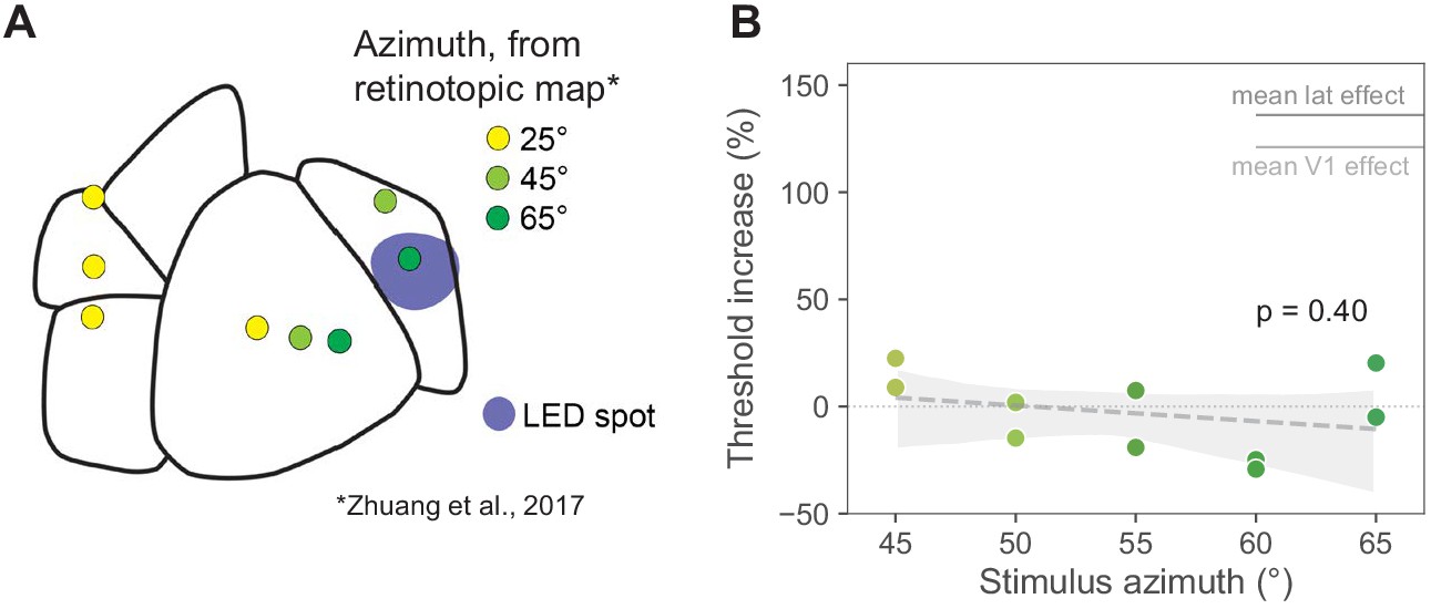
Moving the visual stimulus does not affect PM results.
Stimuli at 0° elevation and 25° azimuth, as we use in most other parts of this work, are represented at the very anterior edge of PM. A stimulus at the same elevation but 45° azimuth is also in the anterior part of PM, just below the PM boundary, and a stimulus at 65° azimuth is closer to the center of PM. All locations based on retinotopic mapping (Zhuang et al., 2017; Garrett et al., 2014). To rule out that PM effects were small because of retinotopic positions, in one animal we performed behavioral inhibition experiments with the stimulus at different positions, ranging from 45° to 65° azimuth, in 5° increments. The results were similar to those seen with a 25° azimuth stimulus: little change in threshold when PM was inhibited, confirming that the small PM effects we found were not due to the retinotopic position of the stimulus. (A) Map of visual areas, LED spot (blue), and predicted retinotopic locations based on Zhuang et al., 2017 and Garrett et al., 2014 (yellow = +25° Az, 0° El; light green = +45° az, 0° el; dark green = +65° az, 0° el). (B) Threshold increases at each stimulus location (N = 2 sessions at each azimuth, N = 10 sessions total). Light intensity was held constant at 0.5 mW/mm2. Average V1 threshold increase at 0.5 mW/mm2 is shown in light gray (111%). Average LM/AL and RL threshold increase at 0.5 mW/mm2 is shown in dark gray (136%). Threshold increase across azimuths (all data shown here) was −3.2 ± 17% (mean ± SD) and did not increase or decrease significantly as the visual stimulus was moved closer to the aligned retinotopic location at +65° azimuth (slope p = 0.40, shaded area: bootstrap 95% CI around least-squares regression). At all azimuths tested in PM, the behavioral effects were significantly smaller than the mean effect observed when inhibiting V1 or lateral areas LM/AL or RL.
Figure 5 with 2 supplements
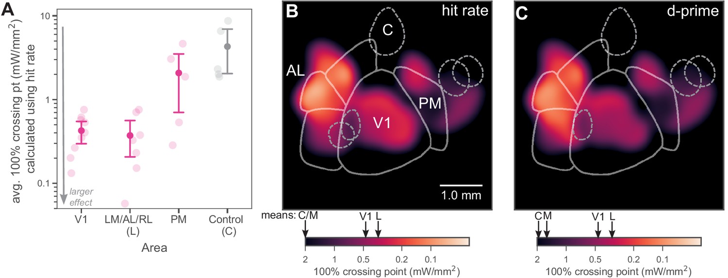
Inhibiting lateral areas produces larger effects than inhibiting PM.
(A) Average 100% crossing point (± bootstrap 95% confidence interval) across all spots within a given area (V1/Lateral/Medial/Control). V1 and lateral areas (LM/AL/RL) require low light intensities to double threshold (mean 0.46, bootstrap 95% CI 0.33–0.58 mW/mm2 and 0.36, CI 0.16–0.59 mW/mm2, respectively). Inhibited areas within PM required much higher intensities (mean 1.7, bootstrap 95% CI 0.67–2.7 mW/mm2) to achieve the same effect, and control areas required even higher intensities (mean 5.1, bootstrap 95% CI 2.3–8.0 mW/mm2). (B) Heatmap of all inhibited spots, colored by hit-rate 100% crossing point. Light intensity required to produce effects in lateral secondary areas is similar to, or larger than, that needed in V1. Mean crossing points from spots within V1, LM/AL, and RL (L), PM (M), and control (C) are represented on color bar with black arrows. (C) Heatmap of all inhibited spots, colored by d′ 100% crossing point. When 100% crossing point is calculated in terms of d′, spots in V1 and lateral areas still require less intensity to double threshold (means 0.68 and 0.48 mW/mm2, respectively) than spots in PM and control areas (means 3.0 and 6.1 mW/mm2, respectively). Mean crossing points, color bar: same notation as in (B).
Figure 5—figure supplement 1
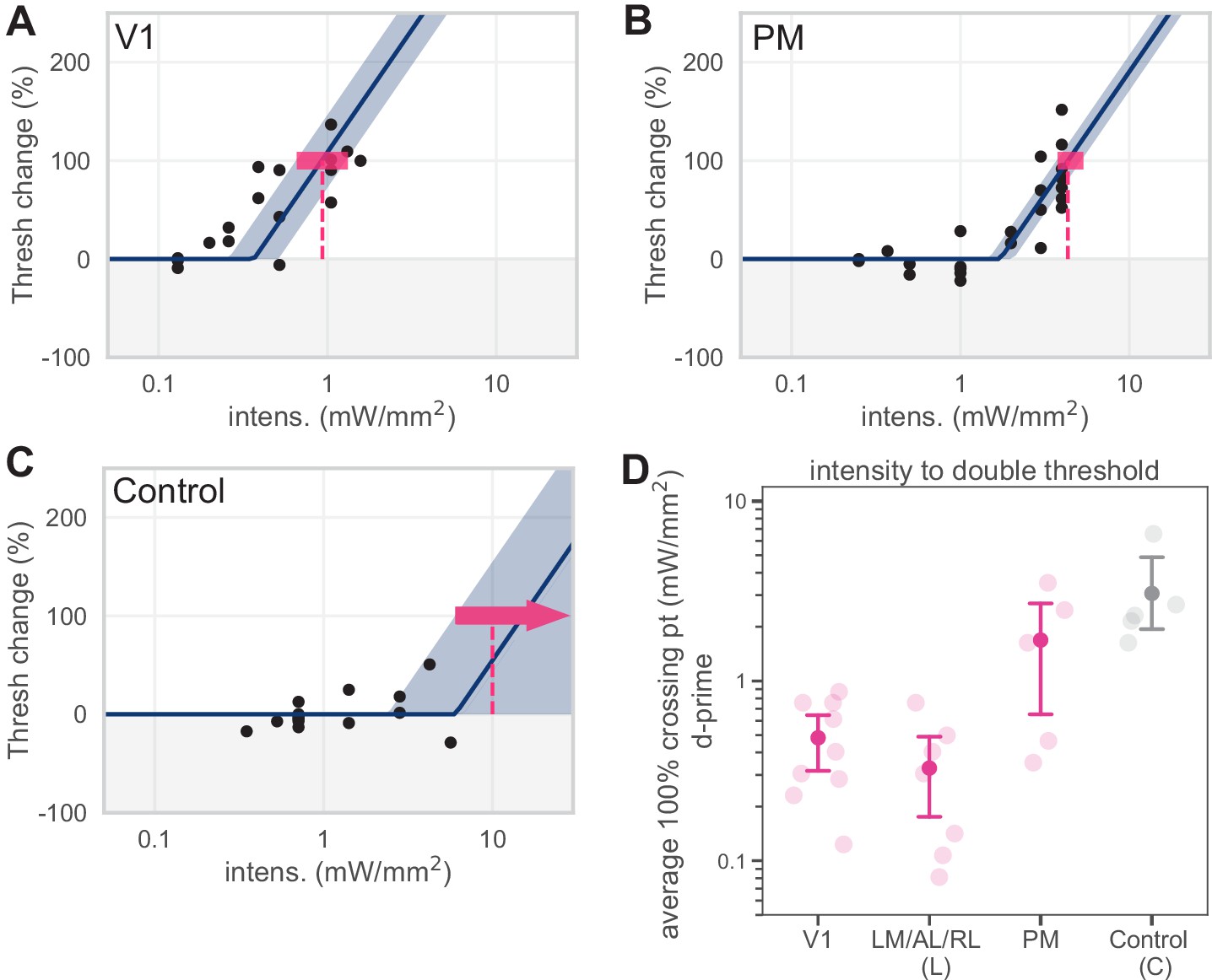
d′ 100% crossing point calculations.
Predicting 100% crossing point using d′ values does not alter behavioral effects. (A–C) Piecewise-linear functions were fit to d′ data in the same manner described in Figure 1—figure supplement 3 to predict the intensity necessary to double sensitivity (the d′ 100% crossing point). (D) Plotting behavioral effects in terms of sensitivity (d′) does not affect our main conclusion that inhibiting lateral areas (LM/AL/RL) produce effects similar to those seen in V1, while inhibiting PM produces effects similar to those seen in control areas.
Figure 5—figure supplement 2
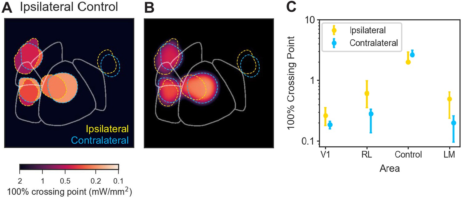
Secondary visual area effects are not motor effects.
Changing the motor response from contralateral to ipsilateral paw produced a similar pattern of behavioral changes. Thus, observed behavioral deficits are primarily sensory, not motor, effects. (A and B) In all other data reported in this work, animals were trained to use the paw contralateral to the inhibited hemisphere to press and release the lever. To determine how effects would change when the motor response modality was changed, we trained one animal to use its ipsilateral paw and inhibited areas matched to those inhibited in a second animal trained to use its contralateral paw. Inhibiting similar areas in the two animals (yellow dashed lines surround spots from animal using its ipsilateral paw, blue dashed lines: contralateral paw) produced similar results. (C) Crossing points (with 95% CIs for the piecewise-linear functions) for the data shown in A and B. There is a trend for the ipsilateral-paw animal to have a mean crossing point larger (i.e. require more power to achieve a similar change in threshold) than the contralateral-paw animal for areas V1, RL, and LM/AL. However, in none of these cases do the thresholds rise to the level of the control data. Therefore, while we cannot rule out that there may be some motor contribution to the inhibition-induced behavioral changes, these experiments show that the effects on performance are primarily non-motor (sensory) effects.
Figure 6 with 3 supplements
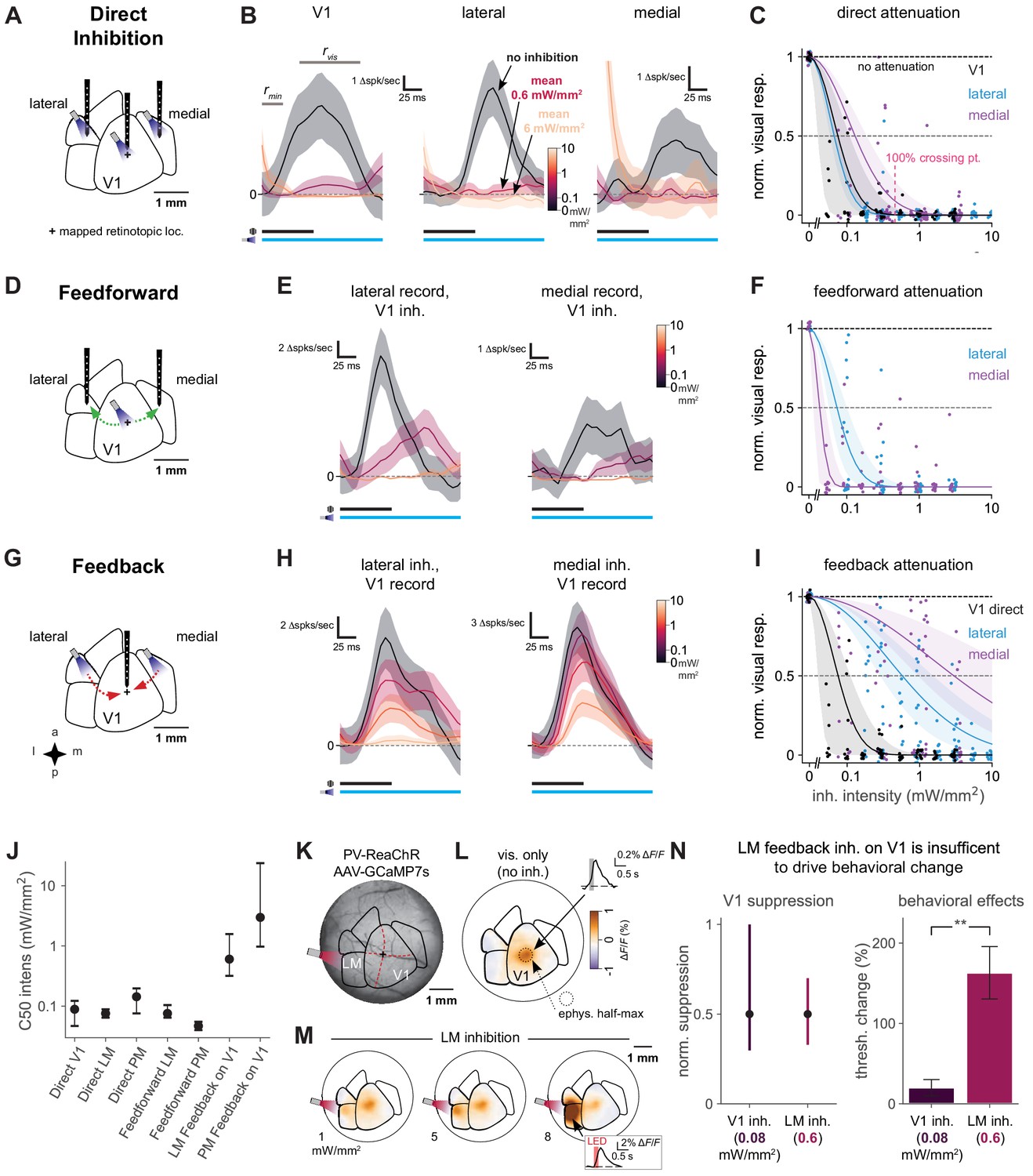
Direct activity reduction in secondary areas, not exclusively feedback suppression onto V1, accounts for degradation of behavioral performance.
(A) Schematic of direct optogenetic inhibition of V1, lateral, and medial areas. Plus sign: visual stimulus at a mapped retinotopic location in V1. (B) Average visual responses in each cortical area with increasing amounts of optogenetic inhibition (0, 0.6, and 6.0 mW/mm2). Responses are subtracted by baseline , a 25 ms period during which optogenetic inhibition has reduced spontaneous neural activity but before visually evoked spikes arrive to the cortex. : visual response period for analysis in C. Black and blue bars: duration of visual stimulus and optogenetic inhibitory stimulus, respectively. Vertical scale bars in panels vary, to more clearly illustrate relative suppression with optogenetic stimulation; quantification in panel C. The rightmost panel shows at the highest power a transient associated with ISN dynamics (Sanzeni et al., 2020, Figure 6—figure supplement 3), which has ended by the time the visual response analysis period begins. V1, lateral, medial panels: N = 14, 6, 7 single units. (C) Summary of direct inhibition effects on visually evoked responses for all intensities. One point is shown for every unit and every intensity level (four to five intensities per unit). Data set for A-I: 11 recording sessions in two animals; 22 electrode penetrations, each with eight recording sites, N = 79 total single units, see Figure 6—figure supplement 3B for electrode positions, see Materials and methods for selection of visually responsive units. Normalized visual response of 1 is no attenuation (black dotted line). Points are jittered slightly in both x and y directions for visual display, including at zero intensity where y = 1 for all points. Pink dotted line: Mean LED intensity for V1 100% behavior threshold change. Solid curves: Gaussian fits, shaded region: 95% CI via bootstrap. 50% suppression level shown by lighter dashed line. (D) Schematic of inhibition of feedforward V1 connections to secondary visual areas (green arrows). (E) Average visual responses measured in lateral areas and PM with increasing optogenetic inhibition applied to V1; conventions as in panel B. Lateral, medial panels: N = 4, 6 single units. (F) Summary of feedforward effects. Conventions as in panel C. (G) Schematic of feedback suppression of V1 during inhibition of secondary visual areas (red arrows). (H) Average visual responses measured in V1 with increasing optogenetic inhibition applied to lateral areas or PM. Lateral, medial panels: N = 26, 16 single units. (I) Summary of direct V1 inhibition versus feedback suppression for all intensities tested. Conventions as in panel C. (J) Intensities (of inhibitory optogenetic stimulus) that generate 50% visual response suppression for all methods of inhibition (direct, feedforward, and feedback) in all areas (V1, lateral areas, and PM). Error bars: 95% CI; all taken from intersection points with colored lines, shaded regions in panels C, F, and I. Higher intensities are required to produce suppression in V1 through feedback than through either direct or feedforward suppression of V1 to other areas. (K) Schematic of GCaMP7s imaging with LM inhibition in a mouse expressing ReaChR in all PV cells (PV-Cre;floxed-ReaChR mouse). (L) GCaMP7s response to flashed Gabor visual stimulus. Fluorescence map image is calculated by taking the frame-by-frame difference, approximating a spike-deconvolution filter; ΔF/F response without differencing is shown in inset. V1 activation (1.9% ΔF/F ± 0.22%, mean ± SEM) is restricted to the retinotopic location of the stimulus. V1 response is significantly greater than zero. (M) Responses to the visual stimulus paired with LM inhibition at three intensities. Increases in activity (orange) in LM/AL likely reflect increased firing of inhibitory neurons expressing ReaChR (inset: LM/AL light response time course has a decay consistent with GCaMP7s offset dynamics). V1 response was not significantly affected by LM inhibition (1.6% ΔF/F ± 0.16%, p for difference = 0.12, Wilcoxon U = 157.0, N1 = 30 trials, N2 = 30, one animal). (N) Intensity of optogenetic stimulation required to suppress V1 activity directly is much less than needed to achieve same suppression by illuminating LM. Intensities in both areas were chosen to produce the same mean suppression. Direct: 0.08 mW/mm2, suppression mean 0.5, 95% CI 0.3–0.9, N = 4 recording sessions. Feedback: 0.6 mW/mm2, suppression mean 0.5, 95% CI 0.4–0.7, N = 6 recording sessions. Behavioral effects at these powers are very different, indicating that behavioral effects of LM suppression arise principally via changing LM responses, not by feedback inhibition of V1 (V1 threshold increase at 0.08 mW/mm2, N = 9 light spots; less than lateral threshold increase at 0.6 mW/mm2, N = 7 spots; Mann–Whitney U = 3.0, one-sided, p < 0.0014). Errorbars in B, E, and H: SEM across trials of average across neurons on each trial.
Figure 6—figure supplement 1
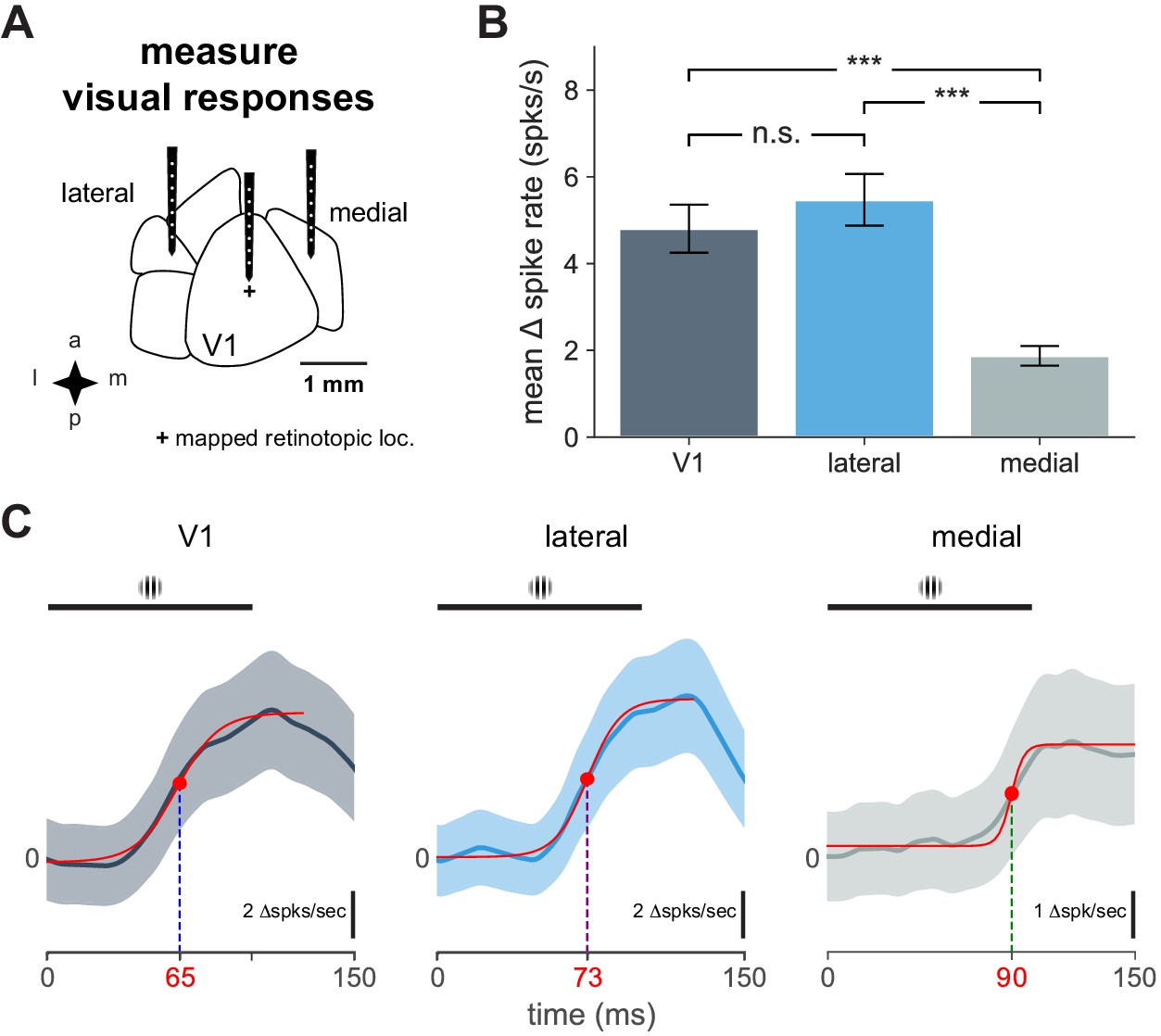
Cortical responses to visual stimulus and response timing.
Characteristics of V1 and secondary visual area cortical responses to visual stimulus and response timing. (A) Schematic of electrophysiological recordings in V1, lateral, and medial areas. ‘+’ indicates visual stimulus at the retinotopic location of the stimulus (identified with hemodynamic imaging) in V1. (B) Mean change in spike rate recorded in indicated cortical area in response to 100 ms flashed Gabor (mean ± SEM: V1, N = 14 units; lateral, N = 10 units; medial, N = 16 units; t-tests: V1-lateral, n.s, t = 0.80, p = 0.49; V1-medial, ***, t = 5.13, p < 0.0001; lateral-medial, ***, t = 6.57, p < 0.0001). (C) Plot of average unit responses (visual stimulus presentation at time = 0) for indicated cortical area with logistic fit (solid red lines). Black bar indicates visual stimulus. Time point for half-maximal response shown for each fit with red dot.
Figure 6—figure supplement 2
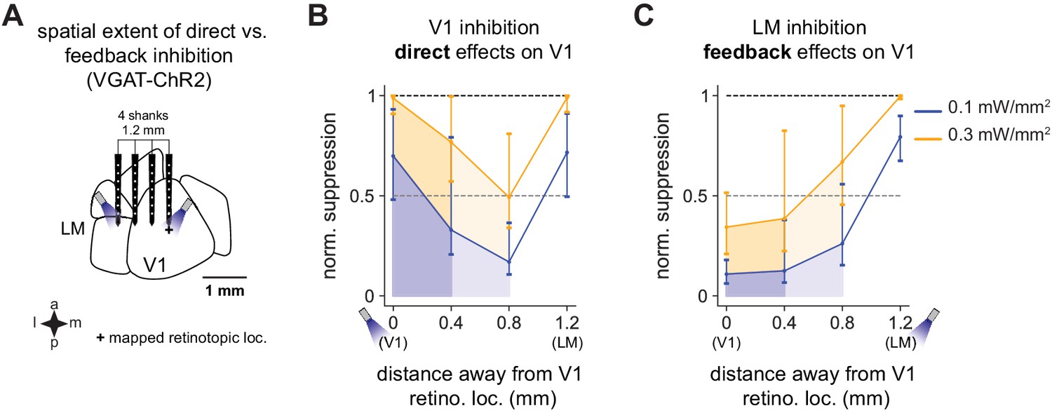
Spatial effects in V1 of feedback vs. direct inhibition.
V1 activity is suppressed substantially more when V1 is directly inhibited than via feedback when LM is inhibited. (A) Schematic of recording setup. A probe with four shanks was placed across V1 and LM. Light was delivered to V1 or LM to cause inhibition, and responses were recorded across all four shanks. (B) Responses in V1 to direct inhibition of V1, showing total normalized suppression (i.e., fraction of the visual response without light that is removed by inhibition; Materials and methods), at distances of 0.4 mm (dark shades) and 0.8 mm (lighter shades) from the recording shank placed at the center of the V1 retinotopic location of the stimulus. Responses are shown at two powers, 0.1 mW/mm2 (blue) and 0.3 mW/mm2 (orange). Responses are normalized to the suppression at the light location (direct suppression) at 0.3 mW/mm2. Normalized suppression increases again at 1.2 mm as the probe crosses into LM and activity is suppressed through inhibition of feedforward connections from V1. (C) Feedback effects on V1 caused by LM inhibition. Same conventions as in B. At all intensities and at all distances, feedback inhibition causes less V1 suppression overall than does direct suppression of V1 (i.e., shaded regions in C versus shaded regions in B).
Figure 6—figure supplement 3
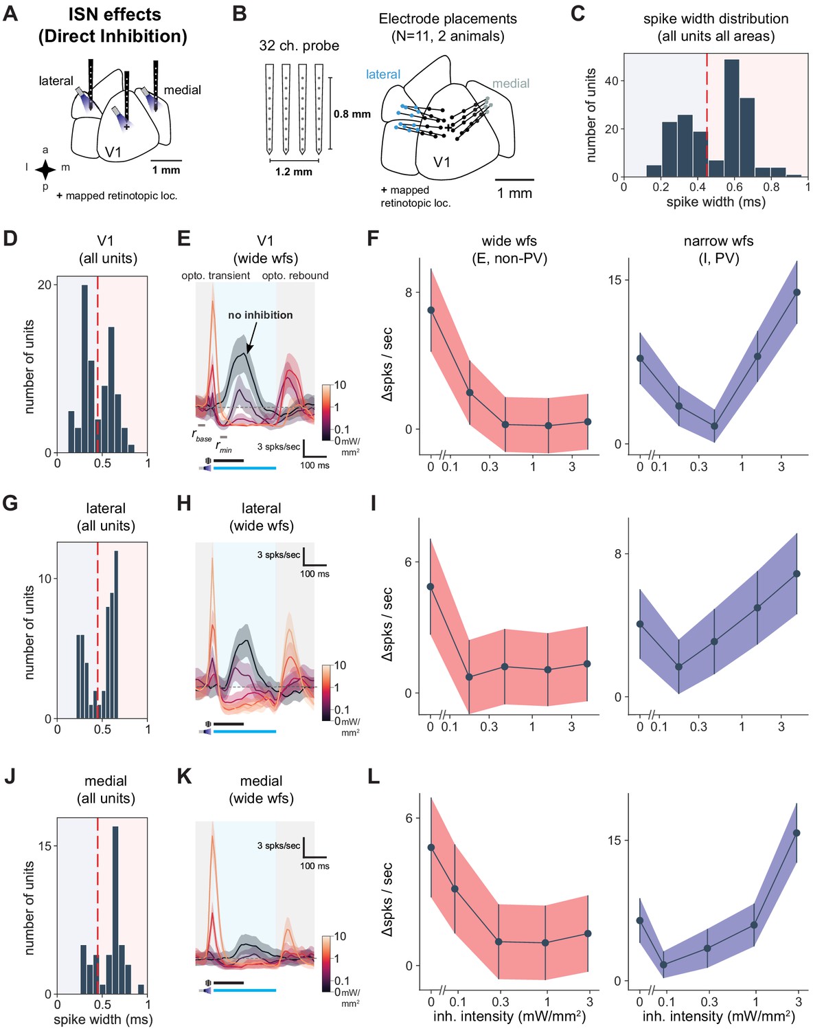
Identification of inhibitory and excitatory units.
V1, lateral areas, and PM display characteristics of inhibition stabilization. (A) Schematic of direct optogenetic inhibition of V1, lateral areas, and PM to examine ISN-related effects. ‘+’ indicates V1 retinotopic location of the visual stimulus, identified with hemodynamic intrinsic imaging (Materials and methods). (B) Schematic of four recording shanks and electrode placements superimposed on cortical area map. Dots: individual shanks. Lines connect shanks recorded in a single experiment. Color: cortical area. (C) Spike width histogram of all units (wide and narrow) across all areas recorded, showing bi-modal distribution, N = 171 units. We used 450 ms as a cutoff between wide and narrow units (red dotted line). The narrow-waveform units reflect mainly inhibitory units, likely dominated by PV+ fast-spiking cells, while wide-waveform units are majority excitatory cells and also some inhibitory neurons (Sanzeni et al., 2020). (D) Spike width histogram of all V1 units (N = 77). (E) Average response of visually responsive wide-waveform (E) V1 units (N = 10) to optogenetic light pulses (blue shaded region) combined with a high-contrast visual stimulus. Some wide-waveform units can be inhibitory (Sanzeni et al., 2020) and would contribute to an initial optogenetic transient (gray shaded region) that rapidly decays. A post-stimulation rebound (gray shaded region) response occurs with the return of cortical activity, especially at high inhibitory stimulation intensities. (F) Average optogenetic responses (Δ spks/s, in panel E) of wide (left, light red) and narrow (right, blue) waveform units recorded in V1 (wide, N = 41 units; narrow, N = 36 units). As expected, wide-waveform (E plus some I) units show little increase at the highest optogenetic power, while narrow-waveform (I) units first decrease, and then increase, their firing rates as inhibitory stimulation intensity is increased. (G) Spike width histogram of all units from lateral sites (N = 51). (H) Average responses of wide-waveform visually responsive lateral units (N = 10 units). Conventions as in E. (I) Optogenetic stimulation responses of wide- (N = 32) and narrow-waveform (N = 19) units in lateral areas. Conventions as in F. (J) Spike width histogram of all units from medial sites (N = 43). (K) Average responses of wide-waveform, visually responsive units in medial areas (N = 8 units). Conventions as in E. (L) Optogenetic stimulation responses of wide- (N = 32) and narrow-waveform (N = 11) units in medial areas. Conventions as in F.
Author response image 1
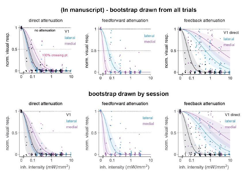
Comparison of 95% confidence intervals when bootstrap groups were drawn from a pool of all trials (top row) or drawn randomly in a nested way: within each individual session holding the unit number within-session constant (bottom row).
Number of bootstrap repetitions in all cases is 10,000. We observed only small differences in error bar sizes among all three classes of inhibition: direct, feedforward, and feedback. Position of points changes from top to bottom row because we randomly jittered each point for display purposes, see Materials and methods.
Tables
Key resources table
| Reagent type (species) or resource | Designation | Source or reference | Identifiers | Additional information |
|---|---|---|---|---|
| Chemical compound, drug | Tamoxifen | Sigma-Aldrich | T5648-5G | |
| Genetic reagent(M. musculus) | VGAT-ChR2-EYFP | The Jackson Laboratory | RRID:IMSR_JAX:014548 | |
| Genetic reagent(M. musculus) | PV-IRES-Cre | The Jackson Laboratory | RRID:IMSR_JAX:008069 | |
| Genetic reagent(M. musculus) | ReaChR-mCitrine | The Jackson Laboratory | RRID:IMSR_JAX:024846 | |
| Genetic reagent(M. musculus) | Ai148 | The Jackson Laboratory | RRID:IMSR_JAX:030328 | |
| Genetic reagent(M. musculus) | Cux2-CreERT2 | MMRRC | RRID:MMRRC_032779-MU | |
| Recombinant DNA reagent | AAV9-hSyn-jGCaMP7s | Addgene | RRID:Addgene_104487 | |
| Software | MWorks | The MWorks Project | mworks.github.io | |
| Other | PEDOT;Poly(3,4-ethylenedioxythiophene) | Sigma-Aldrich | 687553 | |
| Other | PSS;Poly(styrenesulfonate) | Sigma-Aldrich | 243051 | |
| Other | C and B Metabond | Parkell | S380 | |
| Other | Kwik-sil | World Precision Instruments | KWIK-SIL |
Additional files
Download links
A two-part list of links to download the article, or parts of the article, in various formats.
Downloads (link to download the article as PDF)
Open citations (links to open the citations from this article in various online reference manager services)
Cite this article (links to download the citations from this article in formats compatible with various reference manager tools)
Performance in even a simple perceptual task depends on mouse secondary visual areas
eLife 10:e62156.
https://doi.org/10.7554/eLife.62156


