A large accessory protein interactome is rewired across environments
- Department of Biochemistry, Stony Brook University, United States
- Laufer Center for Physical and Quantitative Biology, Stony Brook University, United States
- Joint Initiative for Metrology in Biology, United States
- Department of Genetics, Stanford University, United States
- Department of Applied Mathematics and Statistics, Stony Brook University, United States
- SLAC National Accelerator Laboratory, United States
Figures
Figure 1 with 5 supplements
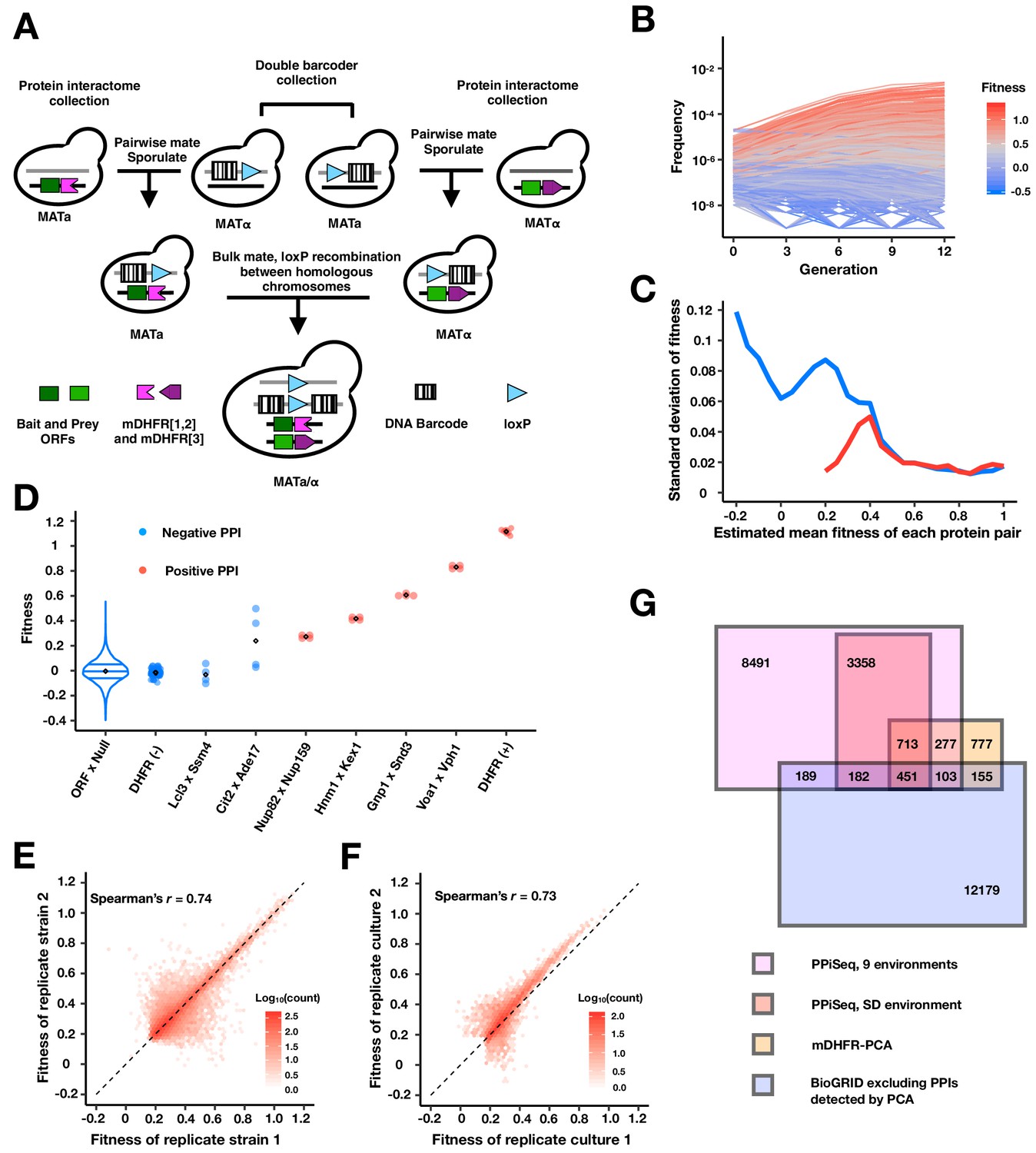
PPiSeq.
(A) A cartoon of PPiSeq yeast library construction. Strains from the protein interactome collection are individually mated to strains from the double barcoder collection and sporulated to recover haploids that contain a mDHFR-tagged protein and a barcode. Haploids are mated as pools. In diploids, expression of Cre recombinase causes recombination between homologous chromosomes at the loxP locus, resulting in a contiguous double barcode that marks the mDHFR-tagged protein pair. (B) Representative double barcode frequency trajectories over twelve generations of competitive growth. Trajectories are used to calculate a quantitative fitness for each double barcoded strain. (C) Standard error of fitness estimates of protein pairs. The blue and red lines represent the median standard error for a sliding window (width = 0.05) of all fitness-ranked protein pairs and of only the positive protein-protein interactions, respectively. (D) Estimated fitness of strains with different double barcodes representing the same protein pair in the same pooled growth. Positive protein pairs are randomly selected within a fitness window. ORF x Null is a violin plot of the fitness distribution of all interactions with a mDHFR fragment that is not tethered to a yeast protein. DHFR(-) is yeast strains that lack any mDHFR fragment. DHFR(+) is yeast strains that contain a full length mDHFR under a strong promoter. (E) Density plot of the fitness of double barcodes that represent the same putative PPI in the same pooled growth. In (B–E), the data in SD environment are used. (F) Density plot of the normalized mean fitness of the same PPI between two pooled growth cultures in SD environment. PPIs detected in either one growth culture are included. (G) Venn diagram of the number of PPIs identified within our search space by PPiSeq in nine environments (magenta), PPiSeq in SD environment (pink), the interactome-scale protein-fragment complementation screen (PCA, yellow), and the BioGRID database excluding any PPIs previously detected by PCA (blue).
Figure 1—figure supplement 1
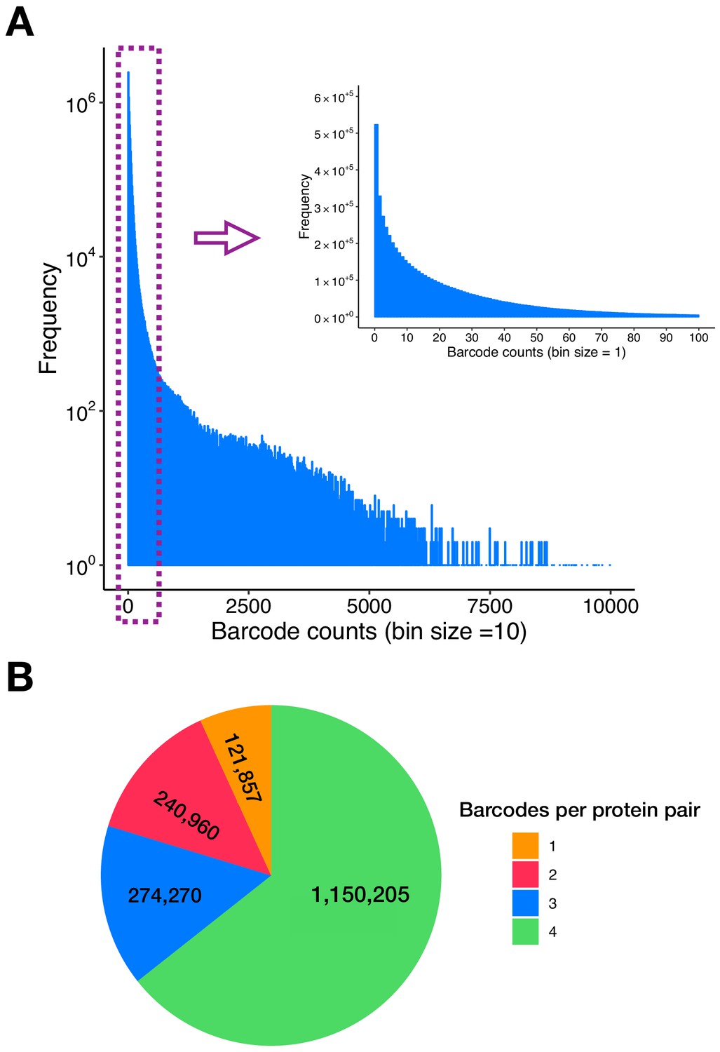
Double barcodes and protein pairs in the PPiSeq library.
(A) Distribution of the initial double barcode count of the PPiSeq library in SD environment at a sequencing depth of 209,899,687 reads. (B) Number of barcodes per protein pair in the PPiSeq library. Spike-in control protein pairs are not included in the plot.
Figure 1—figure supplement 2
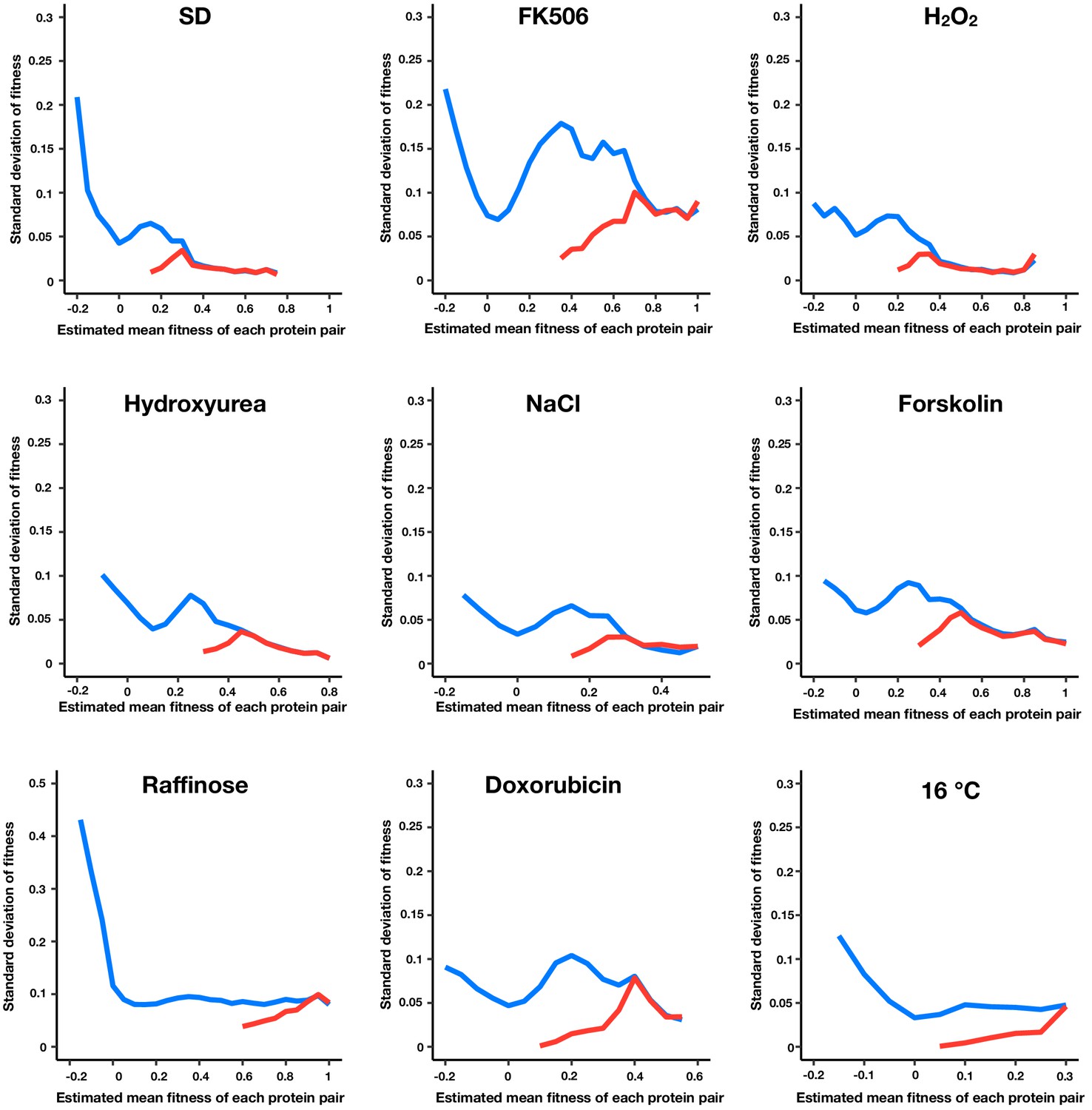
Standard error of fitness estimates of protein pairs in each environment.
The blue and red lines represent the median standard error for a sliding window (width = 0.05) of all fitness ranked protein pairs and of only the positive protein-protein interactions, respectively.
Figure 1—figure supplement 3
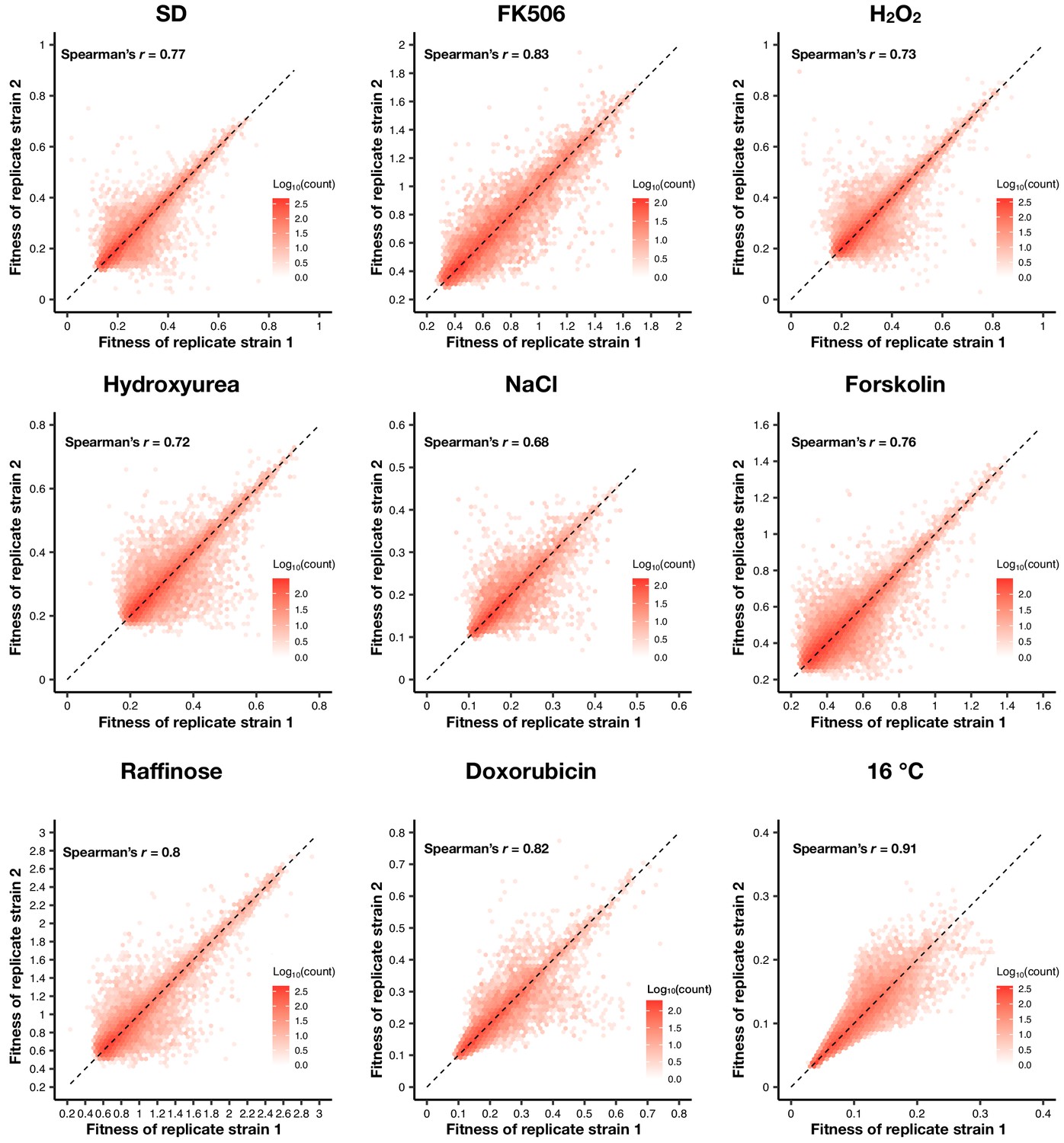
Density plot of the fitness of double barcodes that represent the same positive PPI in the same pooled growth of each environment.
Figure 1—figure supplement 4

Comparison of PPiSeq data in SD condition to other PPI datasets.
(A) Heatmap of overlap coefficients across different datasets. PPiSeq SD1 and PPiSeq SD2 are PPIs identified from two replicate growth cultures. PPiSeq SD-merge is PPIs identfied from the merged data of two replicate growth cultures. PCA is PPIs identified from mDHFR-PCA colony screening (Tarassov et al., 2008). Y2H is PPIs identifed from the latest large-scale yeast-two-hybrid screen (Yu et al., 2008). PRS is a newly constructed ‘bronze standard’ high-confidence positive reference set. Only PPIs within our search space are considered and the numbers are shown under each dataset. (B) Venn diagram of the number of PPIs identified in the two SD PPiSeq replicates and in each of PCA, PRS, or Y2H. (C) Barplot of the overlap coefficients between PPiSeq and other methods for PPIs that do or do not across the two SD PPiSeq replicates.
Figure 1—figure supplement 5

The OD 600 trajectories of DHFR(-) strain in various conditions with and without 0.5 μg/mL methotrexate.
Figure 2
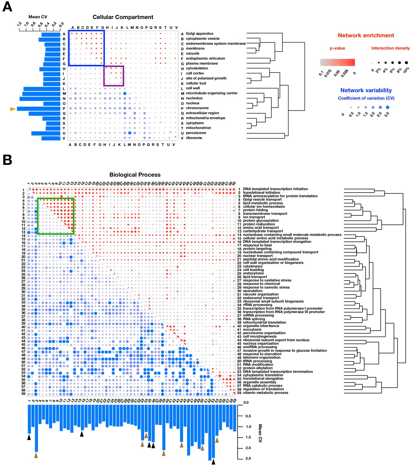
Functional enrichment of PPIs detected by PPiSeq.
PPI enrichment (red) and variability (blue) across environments of gene ontology cellular compartments (A) and biological processes (B). Red node size is the percent of interacting protein pairs (interaction density) observed for a given pair of GO terms and the node color is the p-value of this percent over a random expectation. Blue node size and color are the variability (coefficient of variation, CV) of interaction densities across nine environments tested. GO terms are hierarchically clustered by the interaction density (red dots). Boxes mark frequently interacting and invariable cellular compartments and biological processes involved in membrane transport and protein maturation (blue and green) and cell division (purple). Barplots show the mean CV of interaction densities for each GO term across all other GO terms. Orange, black and brown triangles highlight three different groups of related GO terms: chromosome, transcription, and translation, respectively.
Figure 3 with 6 supplements
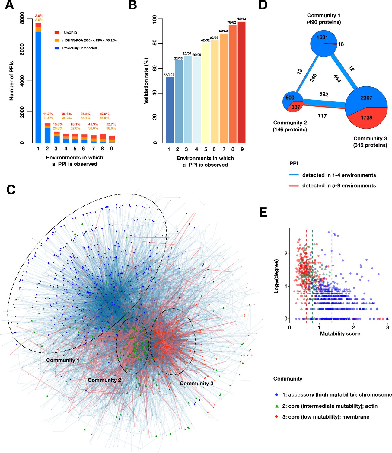
A large accessory protein interactome.
(A) Barplot of PPI number binned by the number of environments in which a PPI is observed. Colors indicate PPIs called by both PPiSeq and BioGRID inclusive of mDHFR-PCA (red), PPIs called by PPiSeq that scored high but were not called by mDHFR-PCA (yellow), and PPIs called by PPiSeq that scored low by mDHFR-PCA (blue). (B) Validation rates of PPIs binned by the number of environments in which a PPI is observed. Validations were performed using OD600 trajectories of clones grown in multi-well plates. (C) Mutable and less mutable PPIs form distinct modules in the network. PPIs that are detected in at least five environments (red edges) form two tight core modules. PPIs that are detected in fewer than five environments (blue edges) form a less connected accessory module. Proteins in different modules are labeled with different shapes and colors. The network uses an edge-weighted spring embedded layout. (D) Number of PPIs within and between each community. PPIs detected in at least or fewer than five environments are shown in red and blue, respectively. The size of the square or circle is proportional to the number of PPIs. The number below each community is the number of proteins within each community. (E) Scatter plot of degrees and mutability scores of proteins in each community.
Figure 3—figure supplement 1
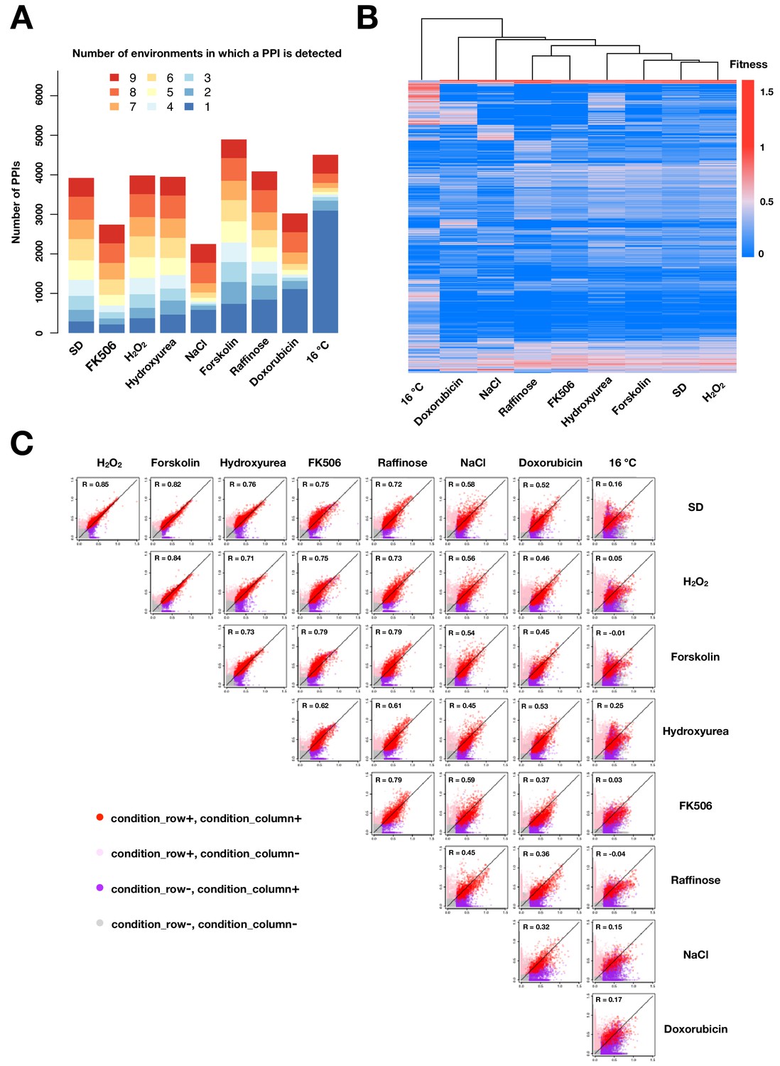
PPIs across conditions.
(A) Barplot of number of PPIs in each environment binned by the number of environments in which a PPI is observed. (B) Heatmap of fitness values of all detected PPIs across different environments. PPIs (rows) and environments (columns) are hierarchically clustered by the fitness values across environments. (C) Scatter plot of mean fitness values of the same PPI across two different growth conditions. Colors indicate in which condition(s) PPIs are called. PPIs that have been detected in at least one environment are shown in (B) and (C). Negative values and missing measurements are replaced with zeros.
Figure 3—figure supplement 2
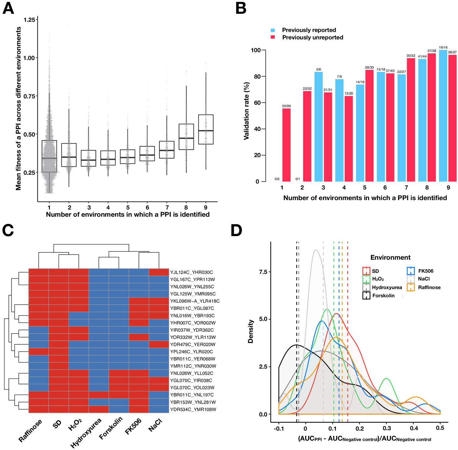
Validating PPIs.
(A) Boxplots and univariate scatterplots of fitness values of PPIs binned by the number of environments in which a PPI is observed. The bottom of each box, the line drawn in the box, and the top of the box represent the 1st, 2nd, and 3rd quartiles, respectively. The whiskers extend to 1.5 times the interquartile range (from the 1st to 3rd quartile). The fitness for each PPI is calculated by taking the mean of the fitness values for all environments where that PPI was detected. (B) Validation rates of PPIs binned by the number of environments in which a PPI is observed. Validations were performed using OD600 trajectories of clones grown in multi-well plates. PPIs that have been previously reported in BioGRID (red) or are previously unreported (blue) are shown. (C) Validation of 20 randomly chosen PPIs that were only detected in SD by PPiSeq. Validations use OD600 trajectories of clones grown in different environments. Red and blue boxes represent positive and negative PPI detection, respectively. (D) Density plot of the increase in the relative area under the growth curve (AUC) against a negative control strain for the 20 PPIs shown in (C). Dashed vertical lines represent the mean AUC increase for an environment.
Figure 3—figure supplement 3
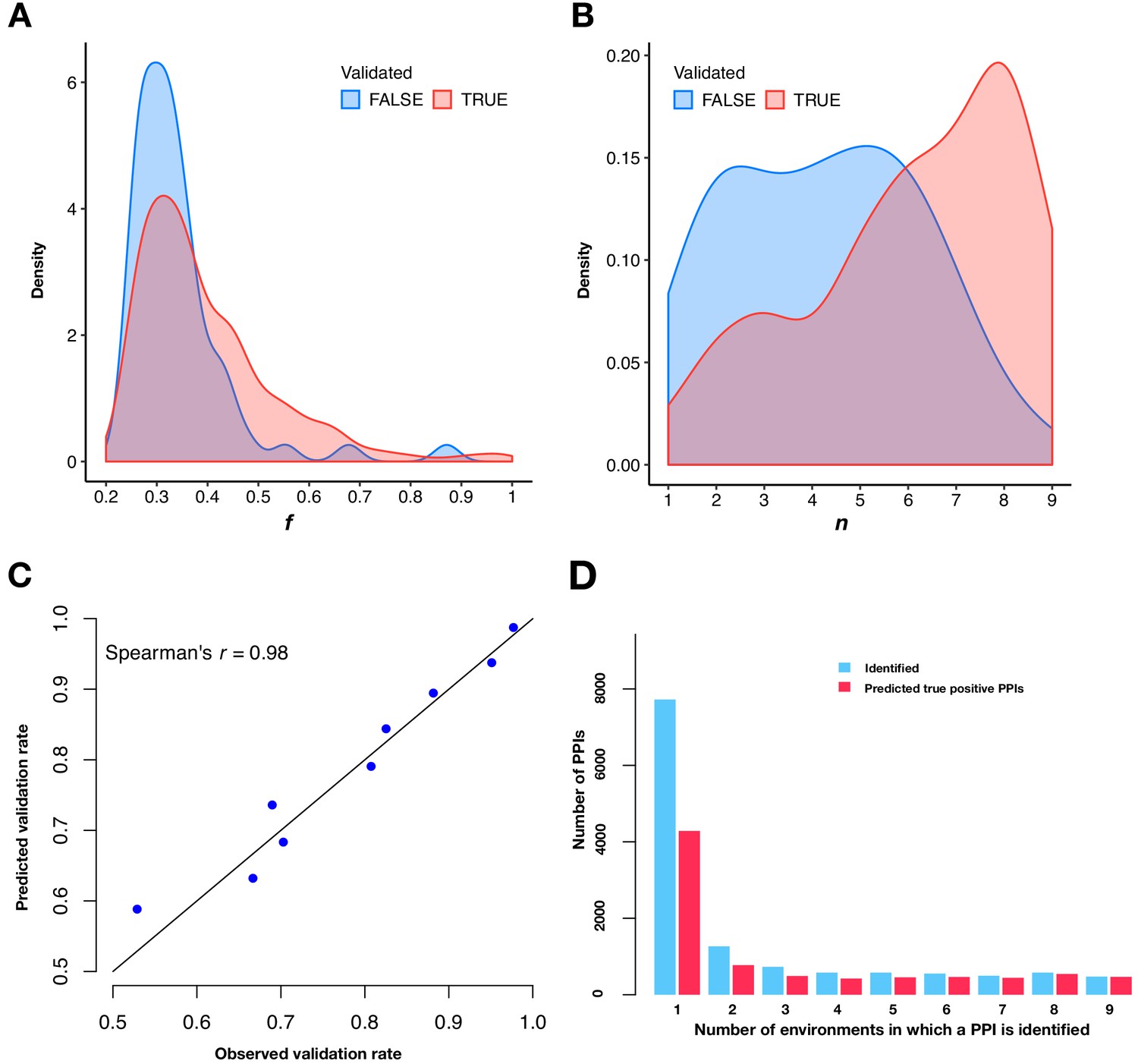
Predicting validation rates.
(A and B) Distributions of mean fitness value (f) and number of environments in which the PPI is detected (n) for validated and unvalidated PPIs. (C) Comparison between observed validation rates and predicted validation rates for 502 PPIs binned by n. Predicted validation rates were calculated using the mean f and n within each bin. (D) Barplot of the PPI number and the predicted true positive PPI number binned by the number of environments in which a PPI is observed.
Figure 3—figure supplement 4
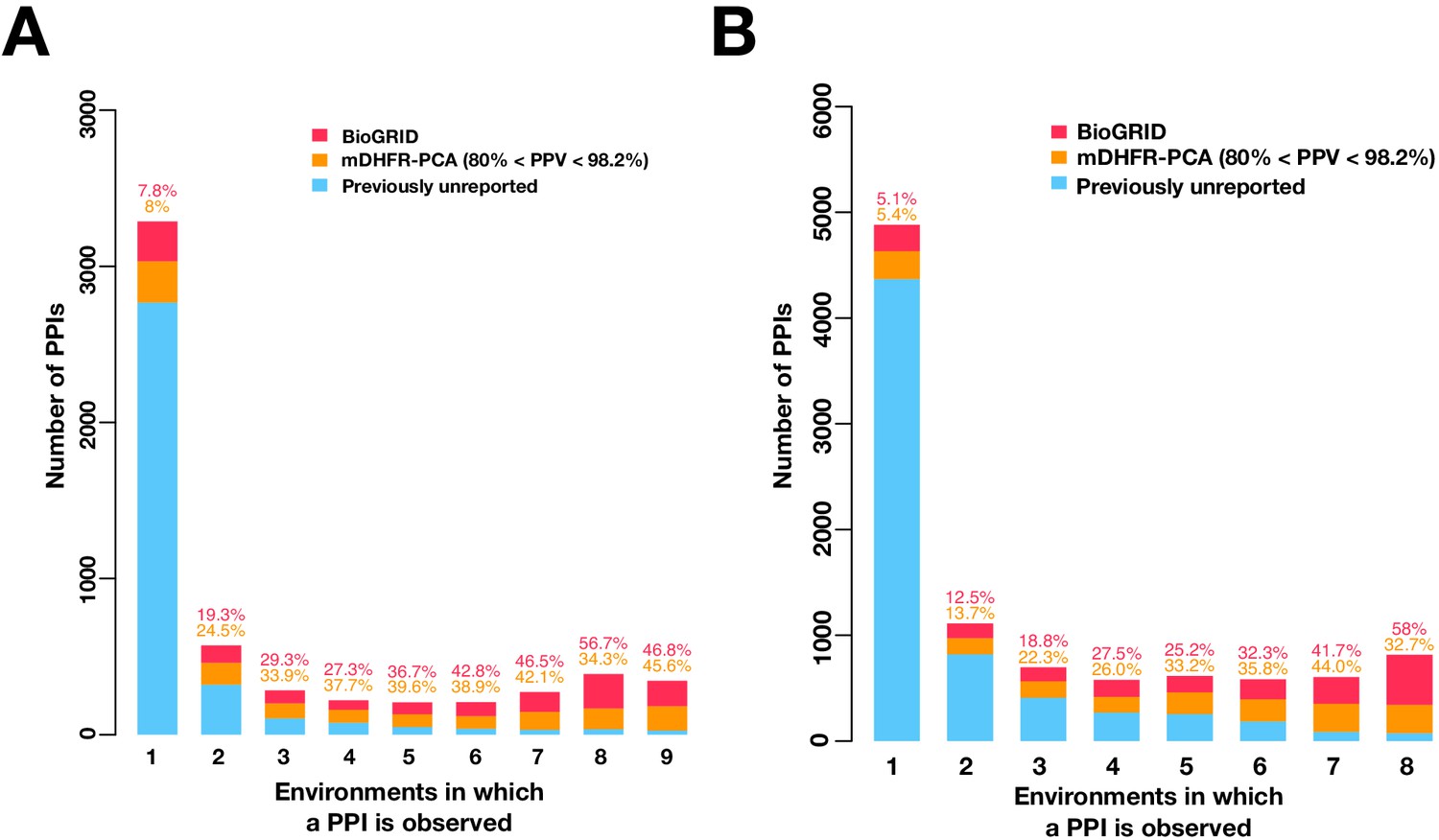
Mutable PPIs outnumber immutable PPIs in higher confidence PPI networks.
Barplot of the PPI number binned by the number of environments in which a PPI is observed in the multi-condition network made by either higher confidence PPI calls (A) or by excluding the 16°C condition (B). Colors indicate PPIs called by both PPiSeq and BioGRID inclusive of mDHFR-PCA (red), PPIs called by PPiSeq that scored high but were not called by mDHFR-PCA (yellow), and PPIs called by PPiSeq that scored low and were not called by mDHFR-PCA (blue).
Figure 3—figure supplement 5
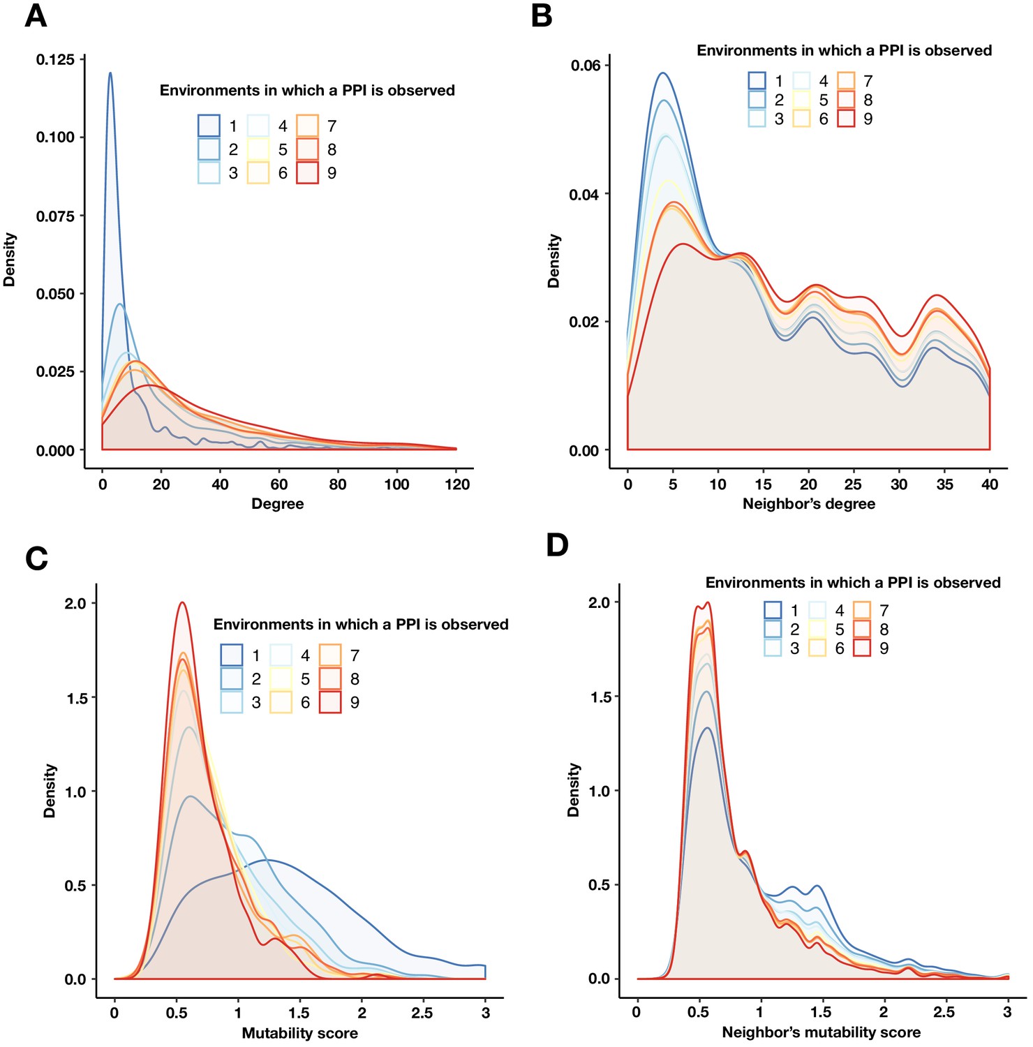
PPIs with a similar mutability are more likely to be connected.
(A) Degree density of proteins binned by the number of environments in which a PPI is detected. (B) Degree density of all proteins that are neighbors of proteins binned by the number of environments in which a PPI is detected. (C) Mutability score density of proteins binned by the number of environments in which a PPI is detected. (D) Mutability score density of all proteins that are neighbors of proteins binned by the number of environments in which a PPI is detected. Any unique protein that participates in a PPI within each bin was counted. The degree (A) and mutability score (C) of a protein were obtained from a multi-environment network that includes all PPIs detected in at least one environment. The degree (B) and mutability score (D) for a target protein’s neighbor was calculated as above, only the interaction between the target protein and its neighbor was first removed.
Figure 3—figure supplement 6
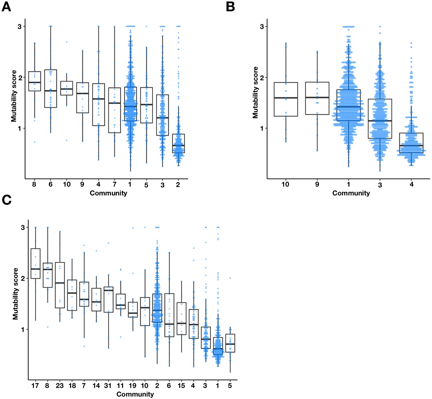
The multi-environment PPI network contains three major communities with different mutability scores.
Boxplots and univariate scatterplots of mutability scores of communities with at least 10 proteins identified by (A) Fast-Greedy (B) Walktrap, and (C) InfoMAP algorithms. The bottom of each box, the line drawn in the box, and the top of the box represent the 1st, 2nd, and 3rd quartiles, respectively. The whiskers extend to 1.5 times the interquartile range.
Figure 4 with 6 supplements
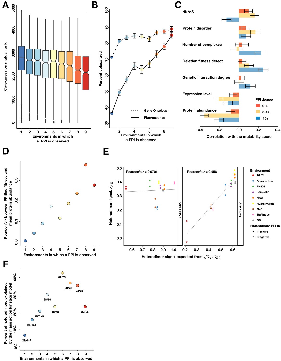
Properties of mutable and less mutable PPIs.
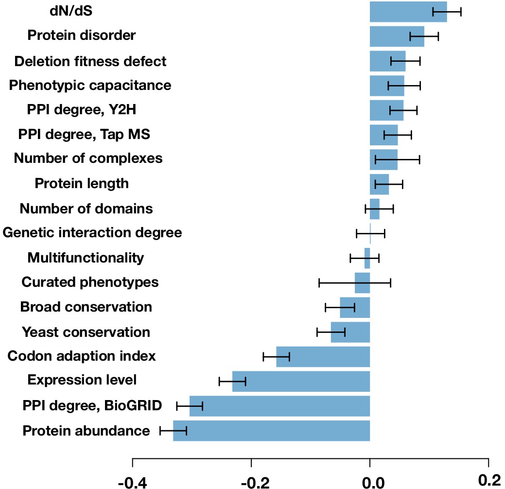
(A) The co-expression mutual rank for PPIs binned by the number of environments in which the PPI is detected. A higher mutual rank means worse co-expression. Notches are the 95% confidence interval for the median, hinges correspond to the first and third quartiles, and whiskers extend 1.5 times the interquartile range. (B) The percent of protein pairs that have been found colocalized by gene ontology (GO Slim, dashed line) and fluorescence (solid line) (Chong et al., 2015). (C) Spearman correlation between the PPI mutability score and other gene features, binned a gene’s PPI degree. In (B) and (C), the error bars are the standard deviation from 1000 bootstrapped data sets. (D) Pearson correlation between a PPI’s fitness and geometric mean abundance of two interacting proteins in Ho et al., 2018, binned by the number of environments in which a PPI is detected. (E) Examples of non-significant (Erv25 x Shr3) and significant (Akr1 x Any1) predictions. Observed heterodimer fitness (SAB) is plotted against the expectation based on the geometric mean of the two constituent homodimer fitnesses (SAA and SBB). (F) Percent of heterodimers whose fitness changes can be significantly predicted by the geometric mean of the two constituent homodimers, binned by the number of environments in which a PPI is observed.
Figure 4—figure supplement 1
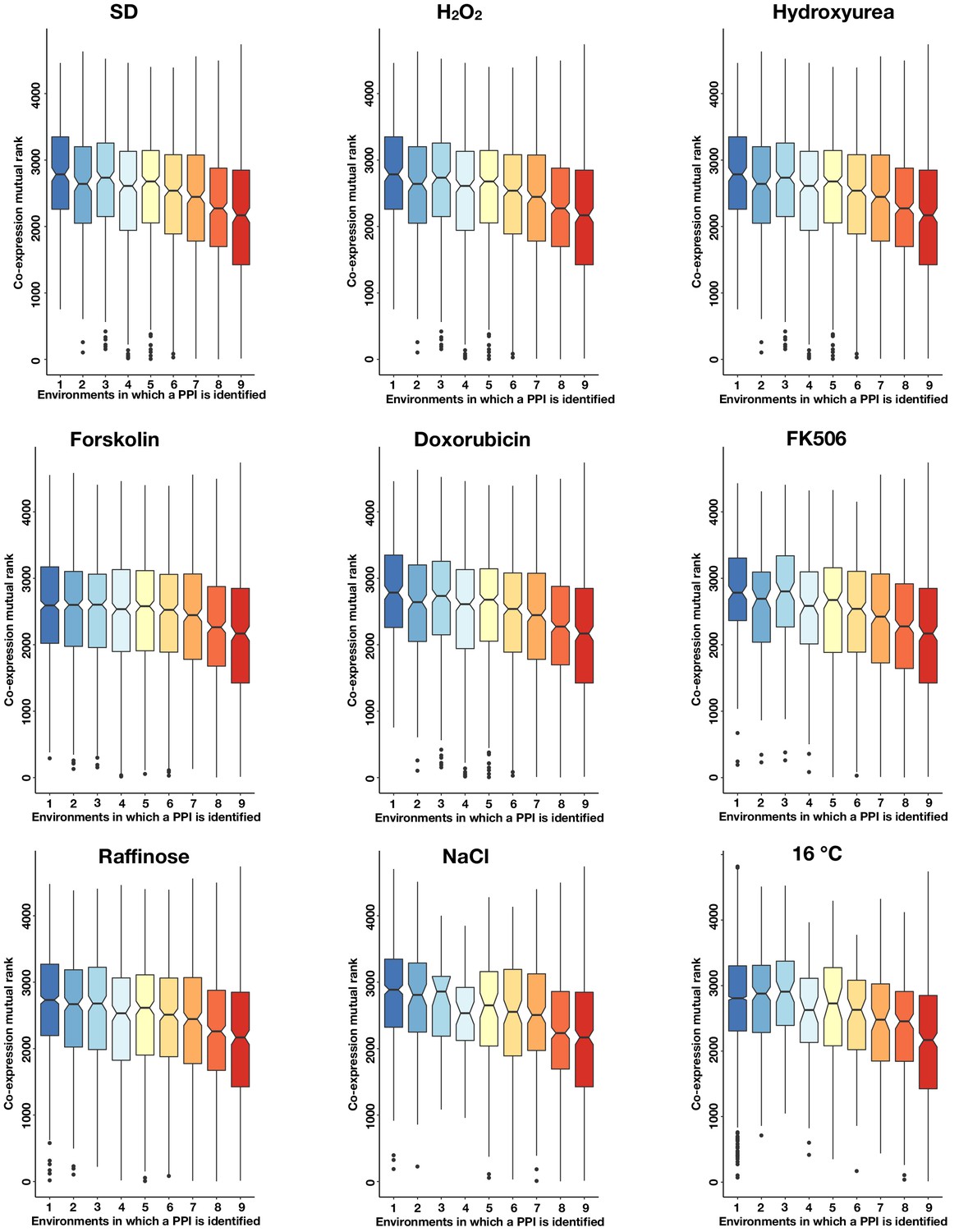
The co-expression mutual rank for PPIs detected in each condition binned by the number of environments in which the PPI is detected.
Notches are the 95% confidence interval for the median, hinges correspond to the first and third quartiles, and whiskers extend 1.5 times the interquartile range.
Figure 4—figure supplement 2
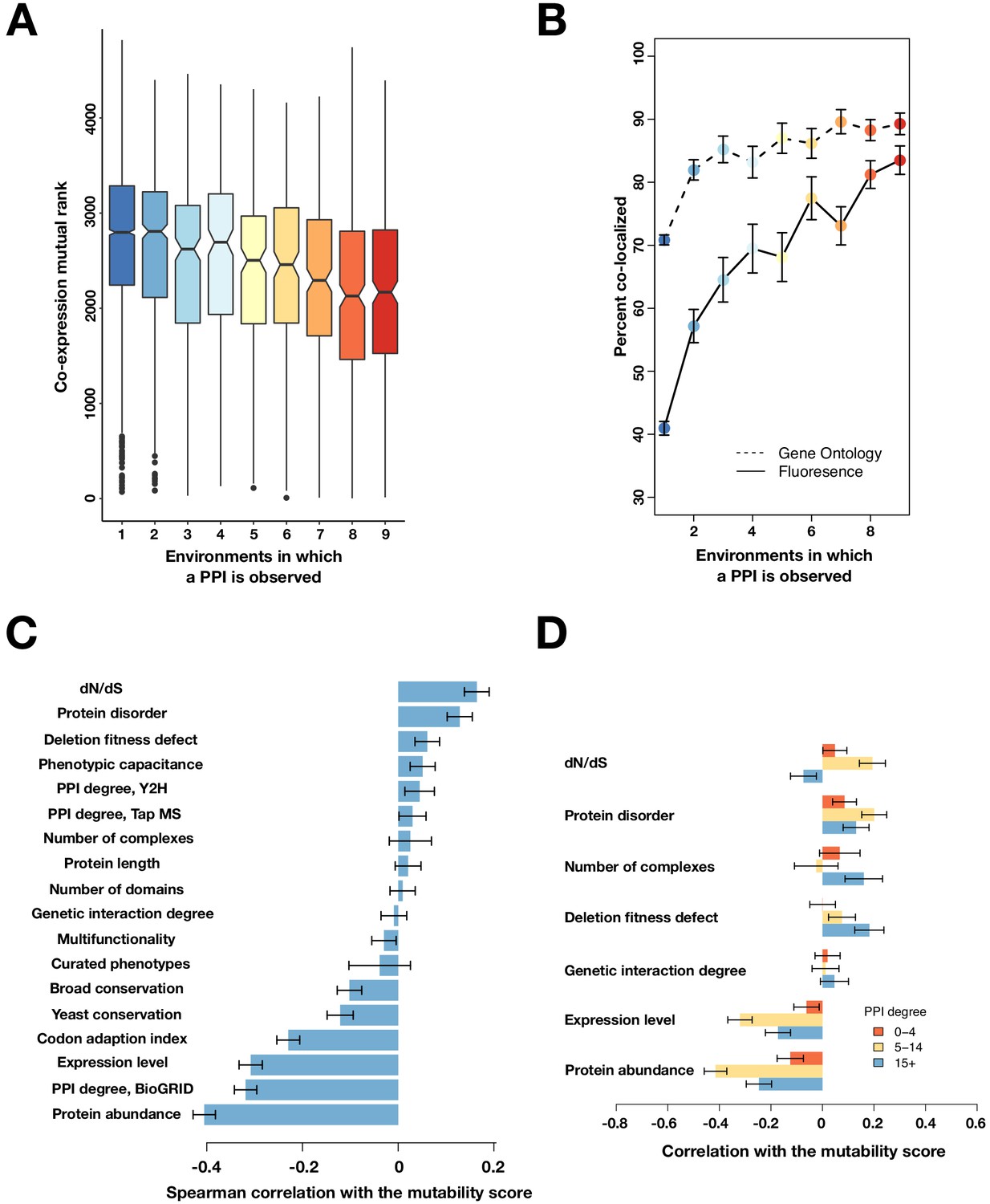
Mutable PPIs and their properties for higher confidence PPI calls.
(A) The co-expression mutual rank for PPIs binned by the number of environments in which the PPI is detected. A higher mutual rank means worse co-expression. Notches are the 95% confidence interval for the median, hinges correspond to the first and third quartiles, and whiskers extend 1.5 times the interquartile range. (B) The percent of protein pairs that have been found colocalized by gene ontology (GO Slim, dashed line) and fluorescence (solid line) (Chong et al., 2015). (C) Spearman correlation between the protein’s mutability score and other gene features. (D) Spearman correlation between the PPI mutability score and other gene features, binned a gene’s PPI degree. In (B–D), the error bars are the standard deviation from 1000 bootstrapped data sets.
Figure 4—figure supplement 3
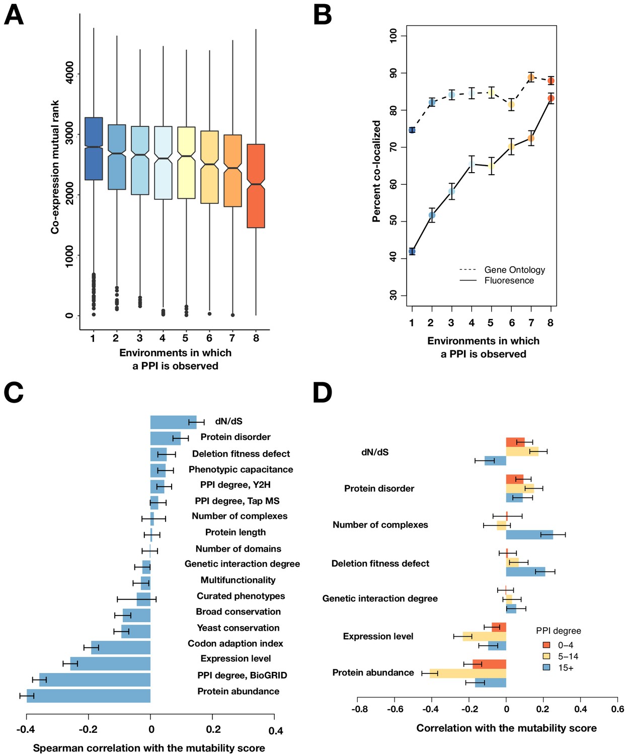
Mutable PPIs and their properties, excluding the 16°C condition.
(A) The co-expression mutual rank for PPIs binned by the number of environments in which the PPI is detected. A higher mutual rank means worse co-expression. Notches are the 95% confidence interval for the median, hinges correspond to the first and third quartiles, and whiskers extend 1.5 times the interquartile range. (B) The percent of protein pairs that have been found colocalized by gene ontology (GO Slim, dashed line) and fluorescence (solid line) (Chong et al., 2015). (C) Spearman correlation between the protein’s mutability score and other gene features. (D) Spearman correlation between the PPI mutability score and other gene features, binned by a gene’s PPI degree. In (B–D), the error bars are the standard deviation from 1000 bootstrapped data sets.
Figure 4—figure supplement 4
Spearman correlation between the protein’s mutability score and other gene features.
The error bars are the standard deviation from 1000 bootstrapped data sets.
Figure 4—figure supplement 5
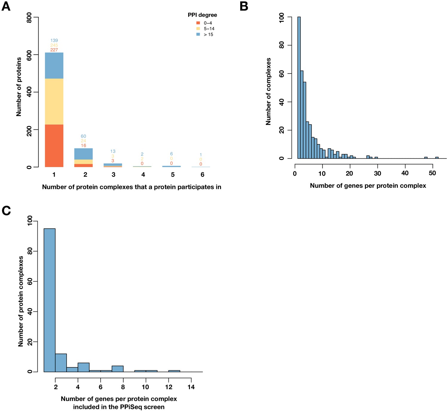
Proteins that participate in multiple complexes are distributed over a wide range of complexes.
(A) Barplot of the number of proteins binned by the number of protein complexes in which a protein participates in. Color represents a protein’s PPI degree. (B) Histogram of number of genes per protein complex (Costanzo et al., 2016). (C) Histogram of number of genes per protein complex for genes included in the PPiSeq screen and involved in at least two protein complexes (Costanzo et al., 2016).
Figure 4—figure supplement 6
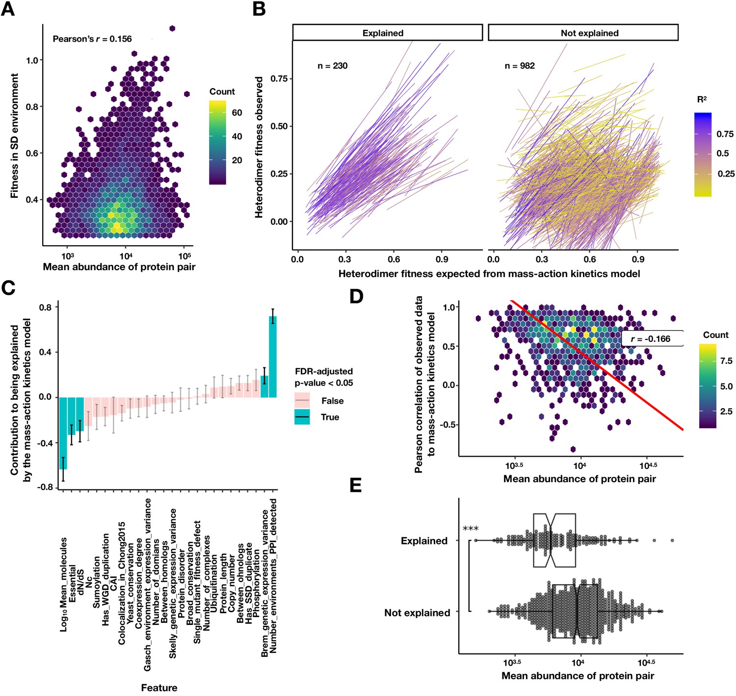
Exploring the relationship of protein abundance, PPI abundance, and PPI mutability.
(A) Density plot of the fitness of a PPI strain in the SD environment against the geometric mean protein abundance from Ho et al., 2018. Colors are the density of points in hexagonal bins. (B) Linear fits to a mass-action kinetic model where the x-axis is the heterodimer PPI fitness expected from the homodimer fitnesses of the constituent proteins, and the y-axis is the measured heterodimer fitness. The left panel contains heterodimers significantly explained by the model that do not require a significant intercept (FDR < 0.05, see Materials and methods). Colors are the R2 of the mass-action kinetics model fit. (C) The coefficients of each scaled feature in a logistic model predicting a good fit to the mass-action kinetics model, as fit by ‘glm’ function in R. (D) Density plot of the geometric mean abundance of a heterodimer pair against the Pearson correlation between the predicted and observed heterodimer fitness across conditions. Colors are the density of points in hexagonal bins. Red line is a Deming regression, r is the Pearson correlation. (E) Explained PPIs are composed of less abundant proteins. Box and dot plot of the mean protein abundance of a heterodimer for PPIs that are explained and not explained by the mass-action kinetics model. Boxplot summarizes the first, second, and third quartiles. ***p<10−9 Wilcoxon signed-rank test.
Figure 5
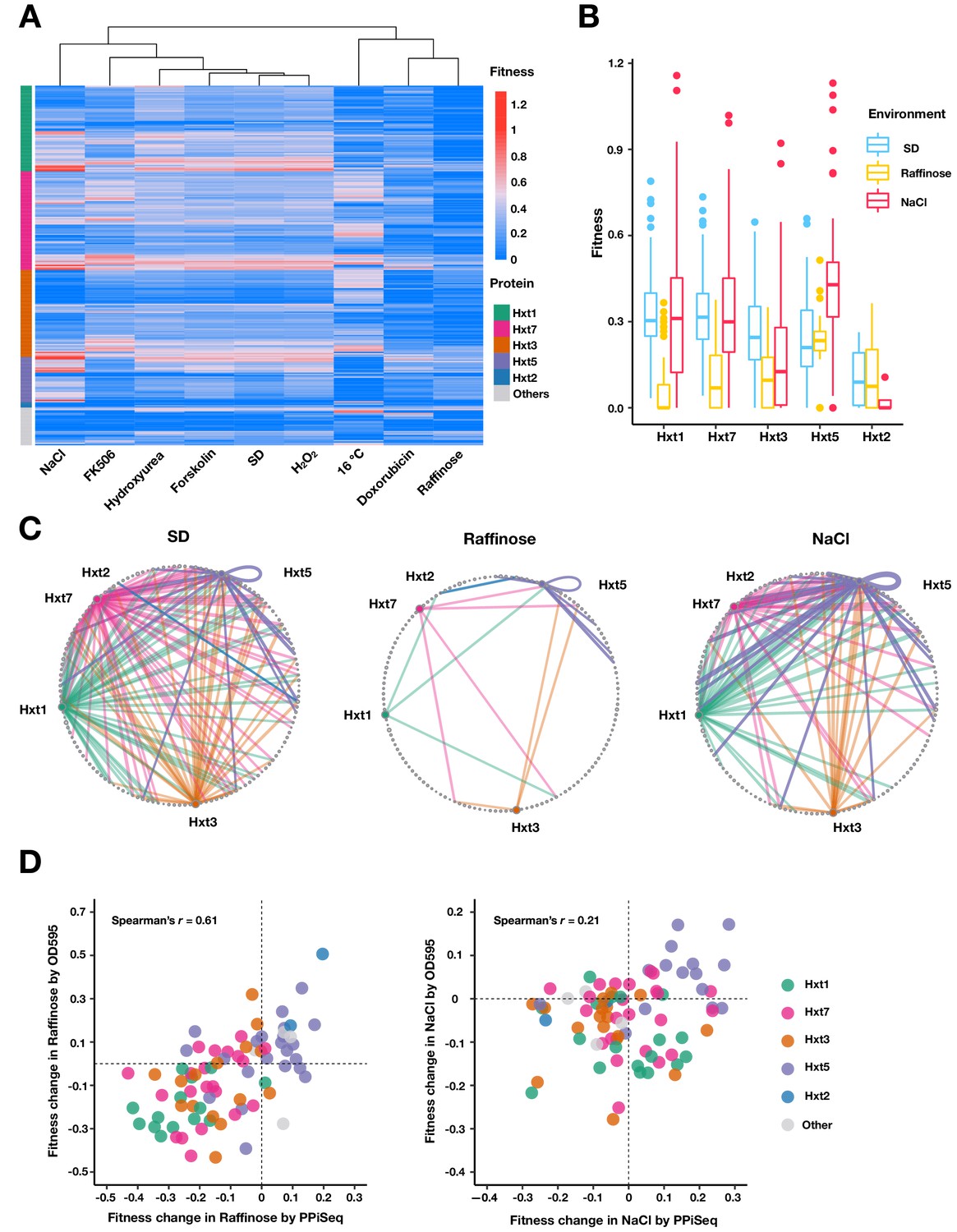
Carbohydrate transport network rewiring as captured by PPiSeq.
(A) Heatmap of abundances (fitnesses) of PPIs involved in carbohydrate transport across different environments. (B) Boxplots of fitnesses of PPIs involving Hxt proteins in SD, Raffinose and NaCl environments. The bottom of each box, the line drawn in the box, and the top of the box represent the 1st, 2nd, and 3rd quartiles, respectively. The whiskers extend to ±1.5 times the interquartile range. (C) Circular network plots of PPIs containing Hxt proteins in SD, Raffinose, and NaCl environments. Nodes are proteins and colors are as in (A). Node size is proportional to its degree in the multi-environment PPI network. Edge width is proportional to abundance in each environment. (D) Scatter plot of fitness changes relative to SD as measured by PPiSeq and clonal growth dynamics for randomly chosen carbohydrate-transport PPIs in Raffinose (80 PPIs) and NaCl (90 PPIs).
Figure 6

The estimated number of true PPIs discovered by PPiSeq using repeated sampling of data in permuted orders of environment addition.
Boxplots summarize the distribution of the number of unique PPIs across permutations. The bottom of each box, the line drawn in the box, and the top of the box represent the 1st, 2nd, and 3rd quartiles, respectively. The whiskers extend to ±1.5 times the interquartile range. Overlayed solid red lines and dashed red lines are the Kindt exact accumulation curves and the bootstrap estimators of the total number of unique PPIs across infinite environments for each simulation, respectively.
Appendix 1—figure 1

Defining a dynamic threshold for PPI calling.
(A) A discrete combination of a fitness threshold (f) and a p-value threshold (p) results in a PPV. Colored lines are fitness and p-value thresholds that result in the same PPV in SD. (B) Density plot of all f and p combinations that result in a PPV of 0.7 using 50 different random reference sets in SD. The black line is the fitted sigmoid model that is used for the dynamic threshold.
Appendix 1—figure 2
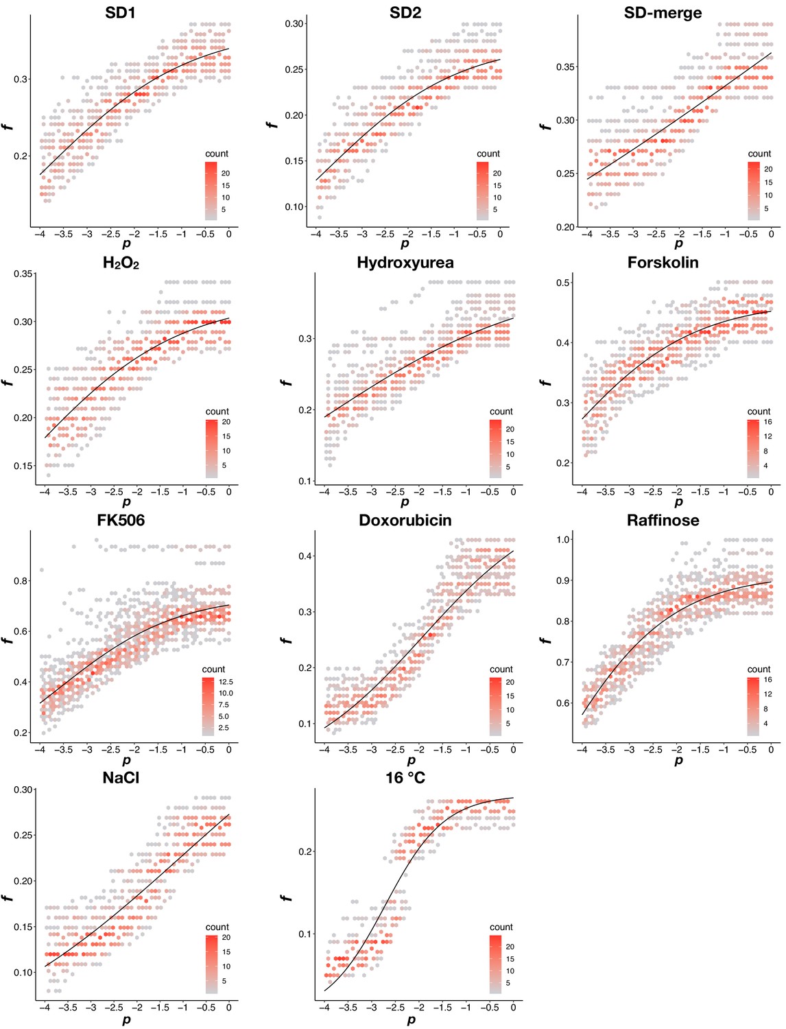
Density plots of the dynamic thresholds in each environment.
Data were split into two groups: p < −4 and p >= −4. For p >= −4, as in Appendix 1—figure 1B, a sigmoidal function was fit to f and p combinations that result in the same PPV value. For p < −4, the fitness threshold was set to equal the minimum fitness value when p >= −4. The dynamic threshold that results in the maximum MCC in each environment was shown in the plot.
Appendix 1—figure 3
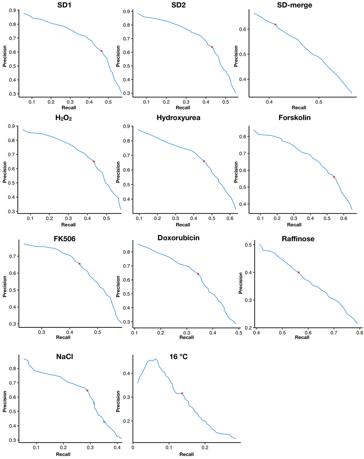
The precision-recall curves of dynamic thresholds in each environment.
Red asterisks mark the thresholds with maximal Matthews correlation coefficients.
Appendix 1—figure 4

Dynamic thresholds (red) of f and p have a higher positive predictive value (PPV) than most discrete combinations (blue).
Points represent the PPVs for dynamic thresholding and for all combinations of discrete fitness and p-value thresholds underlying a constant range of false positive rates obtained from the optimal dynamic threshold in each environment.
Tables
Appendix 1—table 1
Metrics for the dynamic thresholds used in each environment.
‘FPR’: false positive rate; ‘TPR’: true positive rate; ‘PPV’: positive predictive value; ‘MCC’: Matthews correlation coefficient; ‘Detected_PRS(70)”: 70 likely protein interaction pairs in a positive reference set; ‘Detected_RRS(67)”: 67 random pairs in a random reference set (Liu et al., 2019; Yu et al., 2008).
| Optimal dynamic threshold based on the best balance between precision and recall | ||||||||
|---|---|---|---|---|---|---|---|---|
| Environment | Optimal_threshold | FPR | TPR | PPV | MCC | F1_Score | Detected_PRS(70) | Detected_RRS(67) |
| SD1 | 0.7 | 0.00283 | 0.4647 | 0.6075 | 0.5274 | 0.5266 | 20 | 3 |
| SD2 | 0.73 | 0.002315 | 0.4317 | 0.6386 | 0.5214 | 0.5152 | 20 | 2 |
| SD-merge | 0.7 | 0.002473 | 0.4124 | 0.6187 | 0.5012 | 0.4949 | 19 | 3 |
| FK506 | 0.72 | 0.00196 | 0.4352 | 0.6551 | 0.5307 | 0.523 | 20 | 3 |
| H2O2 | 0.73 | 0.002232 | 0.4342 | 0.6517 | 0.5283 | 0.5212 | 20 | 3 |
| Hydroxyurea | 0.74 | 0.00222 | 0.4569 | 0.6613 | 0.5461 | 0.5405 | 19 | 1 |
| NaCl | 0.73 | 0.00145 | 0.2895 | 0.6462 | 0.4292 | 0.3999 | 18 | 1 |
| Forskolin | 0.64 | 0.003727 | 0.5424 | 0.5608 | 0.5476 | 0.5514 | 22 | 2 |
| Raffinose | 0.48 | 0.008105 | 0.5633 | 0.4001 | 0.4688 | 0.4679 | 20 | 2 |
| Doxorubicin | 0.77 | 0.001765 | 0.344 | 0.6425 | 0.4667 | 0.4481 | 18 | 2 |
| 16 °C | 0.41 | 0.00281 | 0.1367 | 0.3164 | 0.203 | 0.1909 | 21 | 3 |
| Arbitrary strict dynamic threshold in each environment | ||||||||
| Environment | Optimal_threshold | FPR | TPR | PPV | MCC | F1_Score | Detected_PRS(70) | Detected_RRS(67) |
| SD-merge | 0.79 | 0.000945201 | 0.283949447 | 0.745351747 | 0.457089253 | 0.411234763 | 17 | 2 |
| FK506 | 0.78 | 0.000978346 | 0.338491296 | 0.747573979 | 0.500365002 | 0.465989091 | 18 | 2 |
| H2O2 | 0.8 | 0.000873036 | 0.306051282 | 0.771675172 | 0.48312128 | 0.438278516 | 17 | 2 |
| Hydroxyurea | 0.8 | 0.000984872 | 0.322118056 | 0.75660523 | 0.490767592 | 0.45186047 | 17 | 1 |
| NaCl | 0.76 | 0.000965072 | 0.237371226 | 0.692789678 | 0.402579452 | 0.353591157 | 18 | 1 |
| Forskolin | 0.77 | 0.000921497 | 0.302696629 | 0.742709167 | 0.471420905 | 0.430101999 | 17 | 1 |
| Raffinose | 0.56 | 0.004453894 | 0.426481481 | 0.479253019 | 0.447039993 | 0.451329915 | 18 | 1 |
| Doxorubicin | 0.82 | 0.000989351 | 0.26916221 | 0.71558061 | 0.435929061 | 0.391182865 | 17 | 2 |
| 16 °C | 0.51 | 0.000900186 | 0.071384083 | 0.432281211 | 0.172518262 | 0.122533747 | 17 | 3 |
Appendix 1—table 2
Summary of promiscuous proteins that interact with an mDHFR fragment that is not tethered to any protein.
Promiscuous and non-promiscuous proteins are represented by 1 and 0, respectively, in each environment.
| PPI | Positive_environme_ number | SD_merge | H2O2 | Hydroxyurea | Doxorubicin | Forskolin | Raffinose | NaCl | FK506 | 16 °C |
|---|---|---|---|---|---|---|---|---|---|---|
| YMR120C | 6 | 1 | 1 | 1 | 0 | 1 | 1 | 0 | 1 | 0 |
| YIL143C | 6 | 1 | 1 | 1 | 0 | 1 | 1 | 1 | 0 | 0 |
| YLL034C | 5 | 1 | 1 | 0 | 1 | 0 | 0 | 1 | 0 | 1 |
| YPL139C | 4 | 1 | 1 | 0 | 0 | 0 | 0 | 1 | 1 | 0 |
| YGR278W | 2 | 0 | 1 | 0 | 0 | 0 | 1 | 0 | 0 | |
| YPL112C | 2 | 0 | 0 | 0 | 1 | 0 | 0 | 1 | 0 | 0 |
| YIL070C | 2 | 0 | 0 | 0 | 1 | 0 | 0 | 0 | 1 | 0 |
| YHL007C | 2 | 0 | 0 | 0 | 1 | 0 | 0 | 0 | 1 | 0 |
| YDR452W | 2 | 0 | 0 | 0 | 1 | 0 | 0 | 0 | 1 | 0 |
| YOL147C | 1 | 0 | 1 | 0 | 0 | 0 | 0 | 0 | 0 | 0 |
| YER087W | 1 | 0 | 0 | 0 | 1 | 0 | 0 | 0 | 0 | 0 |
| YER063W | 1 | 0 | 0 | 0 | 1 | 0 | 0 | 0 | 0 | 0 |
| YOR323C | 1 | 0 | 0 | 0 | 1 | 0 | 0 | 0 | 0 | 0 |
| YNL064C | 1 | 0 | 0 | 0 | 1 | 0 | 0 | 0 | 0 | 0 |
| YKR080W | 1 | 0 | 0 | 0 | 0 | 1 | 0 | 0 | 0 | 0 |
| YJL153C | 1 | 0 | 0 | 0 | 0 | 1 | 0 | 0 | 0 | 0 |
| YDL208W | 1 | 0 | 0 | 0 | 0 | 0 | 0 | 1 | 0 | 0 |
| YLR182W | 1 | 0 | 0 | 0 | 0 | 0 | 0 | 1 | 0 | 0 |
| YPR124W | 1 | 0 | 0 | 0 | 0 | 0 | 0 | 1 | 0 | 0 |
| YHR114W | 1 | 0 | 0 | 0 | 0 | 0 | 0 | 1 | 0 | 0 |
| YDR381C-A | 1 | 0 | 0 | 0 | 0 | 0 | 0 | 1 | 0 | 0 |
| YGR198W | 1 | 0 | 0 | 0 | 0 | 0 | 0 | 1 | 0 | 0 |
| YDR171W | 1 | 0 | 0 | 0 | 0 | 0 | 0 | 1 | 0 | 0 |
| YGR130C | 1 | 0 | 0 | 0 | 0 | 0 | 0 | 1 | 0 | 0 |
| YLL022C | 1 | 0 | 0 | 0 | 0 | 0 | 0 | 1 | 0 | 0 |
| YMR136W | 1 | 0 | 0 | 0 | 0 | 0 | 0 | 1 | 0 | 0 |
| YKL010C | 1 | 0 | 0 | 0 | 0 | 0 | 0 | 1 | 0 | 0 |
| YCR033W | 1 | 0 | 0 | 0 | 0 | 0 | 0 | 1 | 0 | 0 |
| YPL083C | 1 | 0 | 0 | 0 | 0 | 0 | 0 | 1 | 0 | 0 |
| YOR360C | 1 | 0 | 0 | 0 | 0 | 0 | 0 | 1 | 0 | 0 |
| YOR393W | 1 | 0 | 0 | 0 | 0 | 0 | 0 | 1 | 0 | 0 |
| YNL026W | 1 | 0 | 0 | 0 | 0 | 0 | 0 | 1 | 0 | 0 |
| YGR195W | 1 | 0 | 0 | 0 | 0 | 0 | 0 | 1 | 0 | 0 |
| YOR306C | 1 | 0 | 0 | 0 | 0 | 0 | 0 | 1 | 0 | 0 |
| YDL093W | 1 | 0 | 0 | 0 | 0 | 0 | 0 | 1 | 0 | 0 |
| YCR059C | 1 | 0 | 0 | 0 | 0 | 0 | 0 | 1 | 0 | 0 |
| YOL081W | 1 | 0 | 0 | 0 | 0 | 0 | 0 | 1 | 0 | 0 |
| YGR140W | 1 | 0 | 0 | 0 | 0 | 0 | 0 | 1 | 0 | 0 |
| YKL139W | 1 | 0 | 0 | 0 | 0 | 0 | 0 | 1 | 0 | 0 |
| YEL017C-A | 1 | 0 | 0 | 0 | 0 | 0 | 0 | 0 | 1 | 0 |
| YDL112W | 1 | 0 | 0 | 0 | 0 | 0 | 0 | 0 | 1 | 0 |
| YDR057W | 1 | 0 | 0 | 0 | 0 | 0 | 0 | 0 | 1 | 0 |
| YFR001W | 1 | 0 | 0 | 0 | 0 | 0 | 0 | 0 | 0 | 1 |
| YJL124C | 1 | 0 | 0 | 0 | 0 | 0 | 0 | 0 | 0 | 1 |
| YDR151C | 1 | 0 | 0 | 0 | 0 | 0 | 0 | 0 | 0 | 1 |
| YBR057C | 1 | 0 | 0 | 0 | 0 | 0 | 0 | 0 | 0 | 1 |
| YHR146W | 1 | 0 | 0 | 0 | 0 | 0 | 0 | 0 | 0 | 1 |
| YDR379W | 1 | 0 | 0 | 0 | 0 | 0 | 0 | 0 | 0 | 1 |
| YDR513W | 1 | 0 | 0 | 0 | 0 | 0 | 0 | 0 | 0 | 1 |
| YMR227C | 1 | 0 | 0 | 0 | 0 | 0 | 0 | 0 | 0 | 1 |
| YDR420W | 1 | 0 | 0 | 0 | 0 | 0 | 0 | 0 | 0 | 1 |
Author response table 1
Mean fitness in each environment.
| PPI | Environ ment_n umber | SD | H2O2 | Hydroxyurea | Doxorubicin | Forskolin | Raffinose | NaCl | 16℃ | FK506 |
|---|---|---|---|---|---|---|---|---|---|---|
| Rck2_Csh1 | 7 | 0.35 | 0.35 | 0 | 0.20 | 0.54 | 0.74 | 0 | 0.17 | 0.59 |
| Grs1_Pet10 | 9 | 0.44 | 0.39 | 0.34 | 0.25 | 0.65 | 1.19 | 0.2 | 0.16 | 0.95 |
| YDR492W_R pd3 | 3 | 0 | 0.18 | 0 | 0 | 0 | 0 | 0 | 0.17 | 0.61 |
| Mrps35_Bub 3 | 1 | 0.35 | 0 | 0 | 0 | 0 | 0 | 0 | 0 | 0 |
| Positive_cont rol | 9 | 1 | 0.8 | 0.73 | 0.62 | 1.4 | 2.44 | 0.4 | 0.28 | 1.8 |
Additional files
-
Supplementary file 1
Strain losses during barcoding and pool construction.
- https://cdn.elifesciences.org/articles/62365/elife-62365-supp1-v2.xlsx
-
Supplementary file 2
Primers used in the construction of DHFR-fragment control strains.
- https://cdn.elifesciences.org/articles/62365/elife-62365-supp2-v2.xlsx
-
Supplementary file 3
Barcoded haploid DHFR-fragment control strains.
- https://cdn.elifesciences.org/articles/62365/elife-62365-supp3-v2.xlsx
-
Supplementary file 4
Strains in the PPiSeq library.
- https://cdn.elifesciences.org/articles/62365/elife-62365-supp4-v2.xlsx
-
Supplementary file 5
Description of the environmental conditions tested.
Cells were shaken at 220 rpm. In SD, 0.2% DMSO was added as a vehicle control.
- https://cdn.elifesciences.org/articles/62365/elife-62365-supp5-v2.xlsx
-
Transparent reporting form
- https://cdn.elifesciences.org/articles/62365/elife-62365-transrepform-v2.docx
Download links
A two-part list of links to download the article, or parts of the article, in various formats.
Downloads (link to download the article as PDF)
Open citations (links to open the citations from this article in various online reference manager services)
Cite this article (links to download the citations from this article in formats compatible with various reference manager tools)
A large accessory protein interactome is rewired across environments
eLife 9:e62365.
https://doi.org/10.7554/eLife.62365


