Effects of visual inputs on neural dynamics for coding of location and running speed in medial entorhinal cortex
- Center for Systems Neuroscience, Department of Psychological and Brain Sciences, Boston University, United States
Figures
Figure 1 with 1 supplement
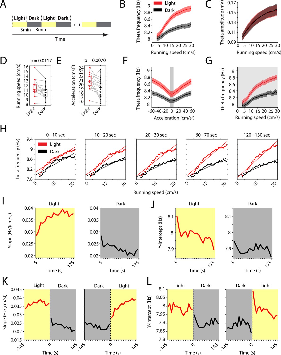
The slope of the local field potential theta frequency to running speed relationship decreases in darkness.
(A) Experimental paradigm. Local field potential (LFP) theta oscillatory activity was recorded in mice freely foraging in a 1 m square open-field environment containing a visual cue card during alternating epochs of illumination by a ceiling light (light) and complete darkness (dark). A typical recording lasted 42 min with 3 min alternating light and dark epochs. (B) Plot of theta frequency vs. running speed shows that the slope of the relationship decreases during darkness. Solid lines show the mean, shaded area show the s.e.m. for n = 15 mice. Data on the light condition are shown in red, data on the dark condition are shown in black and gray. (C) Same as in B, but for theta amplitude. (D) Running speed decreases slightly during darkness. Each data point shows the mean value for one mouse, box plots show mean, 25th and 75th percentiles, gray lines connect data from the same mouse; t = 2,90, df = 14, p=0.0117, Student’s paired t-test. (E) Running acceleration decreases slightly during darkness. Data visualization as in D; t = 3.16, df = 14, p=0.0070, Student’s paired t-test. (F) LFP theta frequency vs. running acceleration relationship is reduced for all acceleration values in complete darkness. Gray background highlights the interval of acceleration values between −5 cm/s2 and 5 cm/s2. (G) LFP theta frequency vs. running speed relationship based on the subset of time points where the running acceleration is near zero in the interval shown in F between −5 cm/s2 and 5 cm/s2. (H–L) Each data point shows the mean across all epochs of the same condition (light or dark) from 78 recording sessions from 14 mice. (H) LFP theta-frequency speed tuning curves for sequential 10 s blocks after the start of light and dark conditions. Straight lines show the results of linear regression. (I–L) Yellow background indicates the light condition; gray background indicates the dark condition. 95% confidence intervals are within the line width. (I, J) Slopes (I) and y-intercepts (J) of the theta frequency vs. running speed relationships for sequential 10 s time bins for the first three minutes in light and dark. (K, L) Left and right panels show 10 s binned slopes (K) and y-intercepts of the theta frequency vs. running speed relationship around the transition points from light to dark and from dark to light, respectively.
Figure 1—figure supplement 1
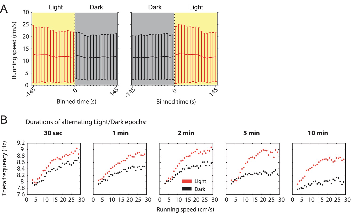
Slow canges in the local field potential theta frequency to running speed relationship as a function of visual inputs can be observed in a single animal and do not correlate with changes in running speed.
(A) Mean running speed as a function of time around the transition points from light to dark or from dark to light plotted in 10 s time bins. Data are shown as mean ± SD across all data points; data from 78 sessions with 3 min alternating epochs of light and dark from 14 mice. (B) Speed tuning curves of local field potential (LFP) theta frequency computed from light (red) or dark (black) epochs of different lengths from the same animal. Note that the gap between speed tuning curves for the light and dark conditions widens with the epochs becoming longer suggesting that speed tuning curves change over time.
Figure 2 with 7 supplements
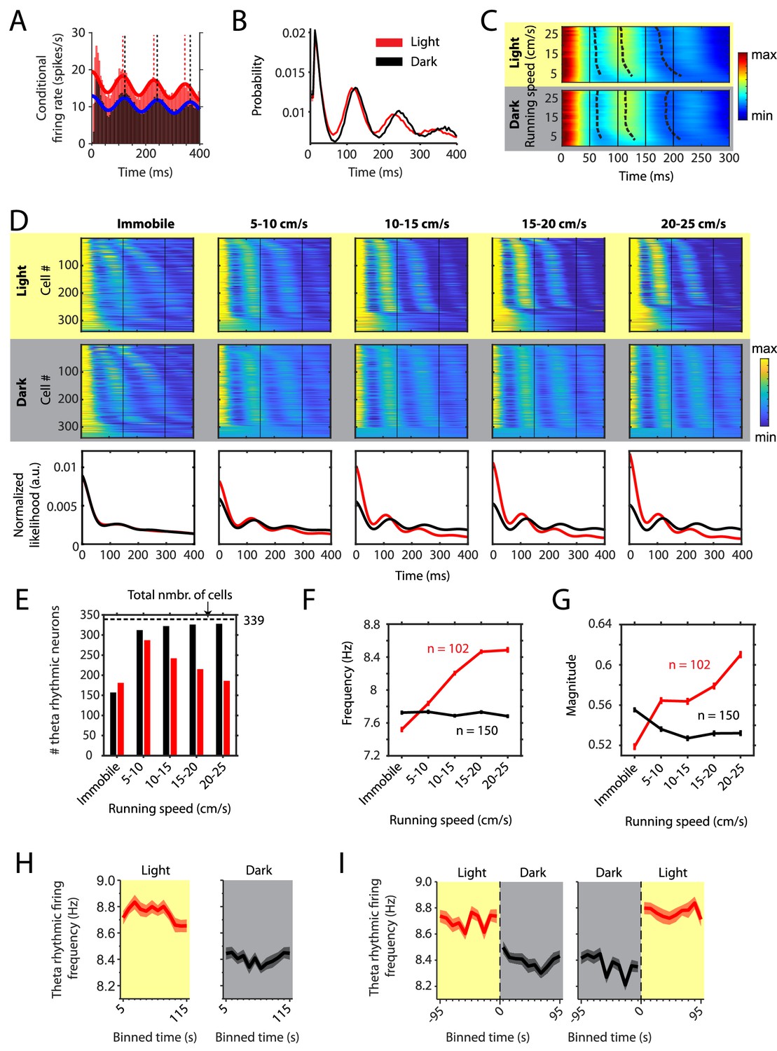
Changes in theta rhythmic firing as a function of running speed differ between light and dark conditions.
Red color or yellow background indicates data on the light condition, black and gray color or gray background indicates data on the dark condition. Figures show data from theta rhythmic neurons from a total of 14 mice. (A) Autocorrelogram of one example neuron showing theta rhythmic firing in light and dark. Solid red and blue lines show the results of the maximum likelihood estimate (MLE) model fit. Vertical dashed lines indicate the positions of the peaks in the autocorrelogram. (B) Mean probability-normalized autocorrelograms for light and dark conditions from n = 342 neurons. s.e.m. is within line width. (C) Figure shows color-coded mean autocorrelogram fits across n = 340 neurons per running speed bin. Speed bins range from 1 ± 4 cm/s to 29 ± 4 cm/s. Dashed lines connect the first peaks in the mean autocorrelogram models. (D) Upper panels show the color coded MLE autocorrelogram models for each of the n = 339 neurons at different running speed intervals. Immobility was defined as running speed <3 cm/s. Neurons are sorted per condition in order of their theta rhythmic firing frequency. Lower row shows the average across autocorrelogram models per condition. Note that higher synchrony across neurons results in higher rhythmicity magnitude in the average across neurons. (E) Number of neurons shown in D with statistically significant spiking rhythmicity at alpha = 0.1 determined by the MLE model for different running speeds in light and dark. (F, G) Longitudinal analysis of frequency (F) and magnitude (G) of theta rhythmic firing of neurons with significant theta rhythmic firing across all running speed bins (light: n = 102 neurons; dark: n = 150 neurons). Data show mean ± s.e.m. (H) Theta rhythmic firing frequency plotted for consecutive 10 s time bins after the start of light and dark conditions. (I) Theta rhythmic firing frequency plotted for 10 s time bins around the transition points from light to dark and from dark to light. Spike time autocorrelograms of theta rhythmic neurons are provided in Figure 2—source data 1.
-
Figure 2—source data 1
Spike time autocorrelograms of the 342 theta rhythmic neurons analyzed for data shown in Figure 2 during light and dark conditions.
- https://cdn.elifesciences.org/articles/62500/elife-62500-fig2-data1-v2.pdf
Figure 2—figure supplement 1
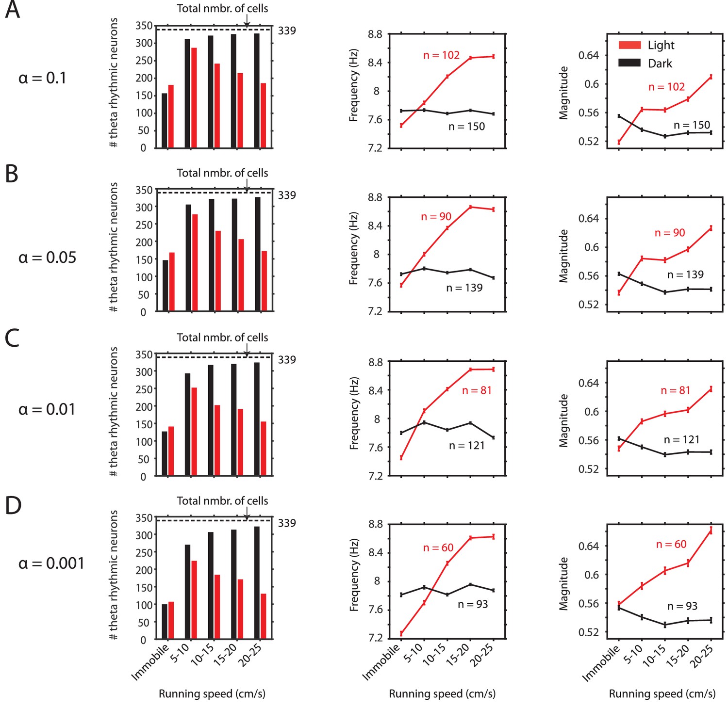
Observed changes in theta rhythmic firing as a function of visual inputs are consistent across a wide range of significance levels chosen to identify theta rhythmic neurons.
(A-D) Results with respect to the number of significant neurons as a function of running speed (first panel) and the frequency (second panel) and magnitude (third panel) of theta rhythmic firing as functions of running speed are consistent across different significance levels alpha for theta rhythmic firing used as threshold criteria for classification of theta rhythmic neurons. Data in second and third panels show mean ± s.e.m.( A) alpha = 0.1, (B) alpha = 0.05, (C) alpha = 0.01, (D) alpha = 0.001.
Figure 2—figure supplement 2
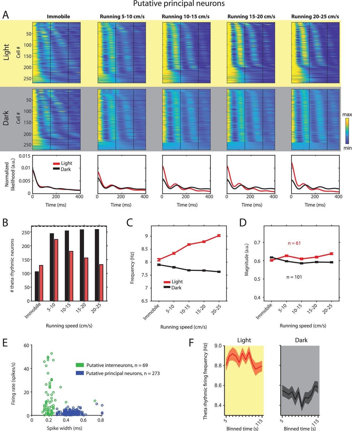
Theta rhythmic firing as a function of running speed and visual inputs in putative principal neurons.
Red color or yellow background indicates data on the light condition, black and gray color or gray background indicates data on the dark condition. (A) Upper panels show the color coded MLE autocorrelogram models for each of n = 270 putative principal neurons at different running speed intervals. Immobility was defined as running speed <3 cm/s. Neurons are sorted per condition in order of their theta rhythmic firing frequency. Bottom row shows the average across autocorrelogram models per condition. Note that higher synchrony across neurons results in higher rhythmicity magnitude in the average across neurons. (B) Number of neurons shown in A with statistically significant spiking rhythmicity at alpha = 0.1 determined by the MLE model for different running speeds in light and dark. (C, D) Longitudinal analysis of frequency (C) and magnitude (D) of theta rhythmic firing of neurons with significant theta rhythmic firing across all running speed bins (light: n = 61 neurons; dark: n = 101 neurons). Data show mean ± s.e.m. (E) Classification of theta rhythmic neurons into putative principal neurons (blue) and putative interneurons (green) based on the spike width and firing rate (see Materials and methods). (F) Theta rhythmic firing frequency plotted for consecutive 10 s time bins after the start of light and dark conditions. Theta rhythmic firing frequency was not correlated with time after start of light (p=0.3688) or dark (p=0.8898) conditions.
Figure 2—figure supplement 3
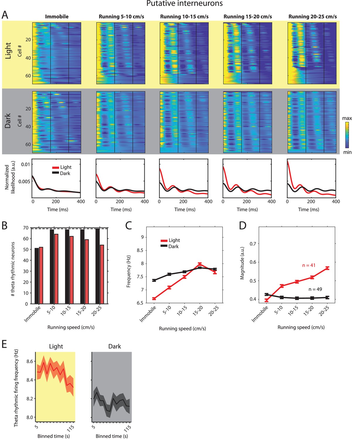
Theta rhythmic firing as a function of running speed and visual inputs in putative interneurons.
Red color or yellow background indicates data on the light condition, black and gray color or gray background indicates data on the dark condition. (A) Upper panels show the color coded MLE autocorrelogram models for each of the n = 69 putative interneurons at different running speed intervals. Immobility was defined as running speed <3 cm/s. Neurons are sorted per condition in order of their theta rhythmic firing frequency. Bottom row shows the average across autocorrelogram models per condition. Note that higher synchrony across neurons results in higher rhythmicity magnitude in the average across neurons. (B) Number of neurons shown in A with statistically significant spiking rhythmicity at alpha = 0.1 determined by the MLE model for different running speeds in light and dark. (C, D) Longitudinal analysis of frequency (C) and magnitude (D) of theta rhythmic firing of neurons with significant theta rhythmic firing across all running speed bins (light: n = 41 neurons; dark: n = 49 neurons). Data show mean ± s.e.m. (E) Theta rhythmic firing frequency plotted for consecutive 10 s time bins after the start of light and dark conditions. Theta rhythmic firing frequency was negatively correlated with time after start of light (p=0.0008) or dark (p=0.0452) conditions.
Figure 2—figure supplement 4
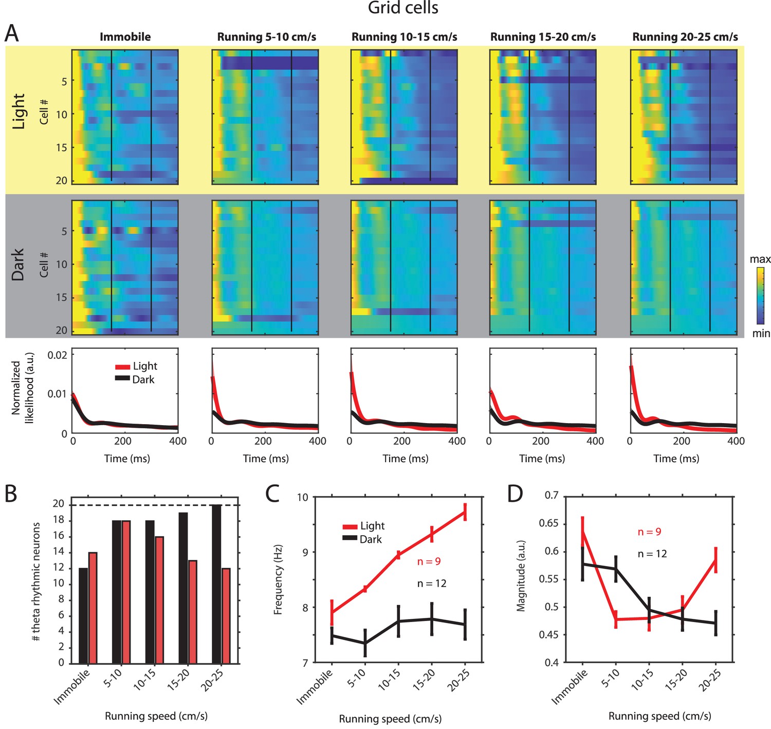
Changes in theta rhythmic firing as a function of running speed and visual inputs in theta rhythmic grid cells.
Red color or yellow background indicates data on the light condition, black and gray color or gray background indicates data on the dark condition. (A) Upper panels show the color coded MLE autocorrelogram models for each of n = 20 theta rhythmic grid cells at different running speed intervals. Immobility was defined as running speed <3 cm/s. Neurons are sorted per condition in order of their theta rhythmic firing frequency. Bottom row shows the average across autocorrelogram models per condition. (B) Number of neurons shown in A with statistically significant spiking rhythmicity at alpha = 0.1 determined by the MLE model for different running speeds in light and dark. (C, D) Longitudinal analysis of frequency (C) and magnitude (D) of theta rhythmic firing of neurons with significant theta rhythmic firing across all running speed bins (light: n = 9 neurons; dark: n = 12 neurons). Data show mean ± s.e.m. As shown for all principal neurons (Figure 2—figure supplement 2 and Tables 1 and 2), the frequency of theta rhythmic firing increased as a function of running speed during the light condition (slope = 0.0928, CI = [0.0461 0.1395], t = 4.0058, df = 43, p=0.0002, linear mixed effects model) but not during the dark condition (slope = 0.0168, CI = [–0.0265 0.0601], t = 0.7764, df = 58, p=0.4407, linear mixed effects model), and the difference between slopes in light and dark conditions was significant (slopeLight–Dark = –0.0760, CI = [–0.1385 –0.0135], t = –2.4125, df = 101, p=0.0176, linear mixed effects model). In contrast, the magnitude of theta rhythmic firing did not change as a function of running speed during the light condition (slope = –0.0017, CI = [–0.0091 0.0057], t = –0.4669, df = 43, p=0.6430, linear mixed effects model). The magnitude of theta rhythmic firing decreased slightly as a function of running speed during darkness (slope = –0.0061, CI = [–0.0120 –2.0430], t = –2.0710, df = 58, p=0.0428, linear mixed effects model) but the slope during darkness was not significantly different from the slope in the light condition (slopeLight–Dark = –0.0044, CI = [–0.0136 0.0049], t = –0.9399, df = 101, p=0.3495, linear mixed effects model).
Figure 2—figure supplement 5
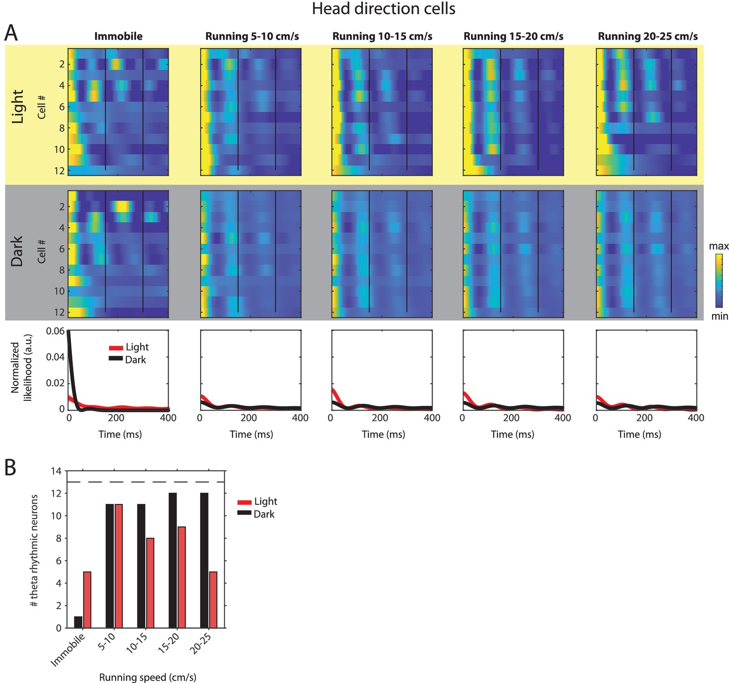
Changes in theta rhythmic firing as a function of running speed and visual inputs in theta rhythmic head direction cells.
Red color or yellow background indicates data on the light condition, black and gray color or gray background indicates data on the dark condition. (A) Upper panels show the color coded MLE autocorrelogram models for each of n = 12 theta rhythmic head direction cells at different running speed intervals. Immobility was defined as running speed <3 cm/s. Neurons are sorted per condition in order of their theta rhythmic firing frequency. Bottom row shows the average across autocorrelogram models per condition. (B) Number of neurons shown in A with statistically significant spiking rhythmicity at alpha = 0.1 determined by the MLE model for different running speeds in light and dark. A longitudinal analysis of changes in frequency or magnitude of theta rhythmic firing as a function of running speed could not be performed because the number of neurons with significant theta rhythmic modulation across all running speed bins was smaller than three in light and dark conditions.
Figure 2—figure supplement 6
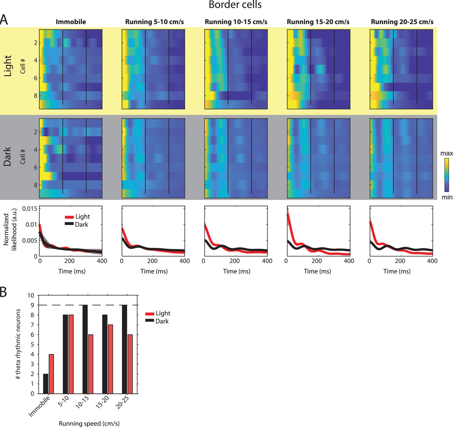
Changes in theta rhythmic firing as a function of running speed and visual inputs in theta rhythmic border cells.
Red color or yellow background indicates data on the light condition, black and gray color or gray background indicates data on the dark condition. (A) Upper panels show the color coded MLE autocorrelogram models for each of n = 9 theta rhythmic border cells at different running speed intervals. Immobility was defined as running speed <3 cm/s. Neurons are sorted per condition in order of their theta rhythmic firing frequency. Bottom row shows the average across autocorrelogram models per condition. (B) Number of neurons shown in A with statistically significant spiking rhythmicity at alpha = 0.1 determined by the MLE model for different running speeds in light and dark. A longitudinal analysis of changes in frequency or magnitude of theta rhythmic firing as a function of running speed could not be performed because the number of neurons with significant theta rhythmic modulation across all running speed bins was smaller than three in light and dark conditions.
Figure 2—figure supplement 7
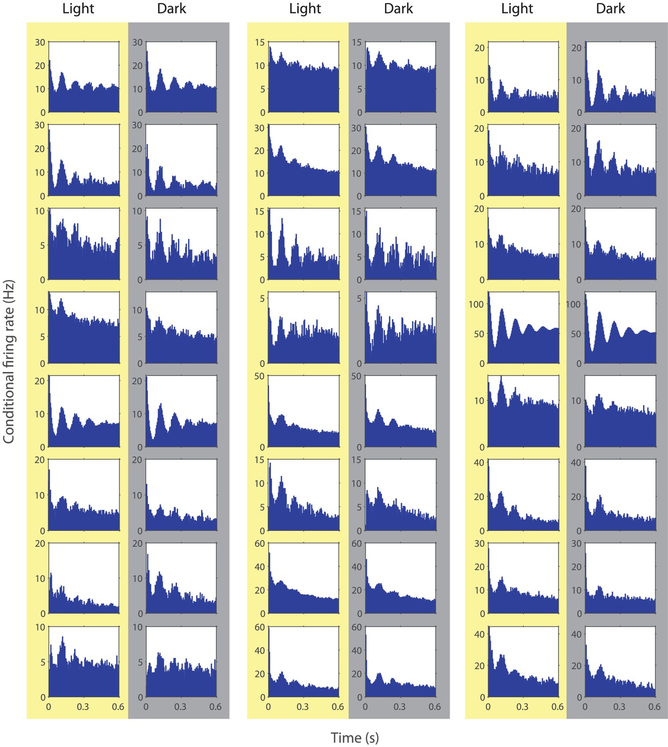
Spike time autocorrelograms of randomly picked 24 theta rhythmic neurons showing theta rhythmic spiking during the light and dark condition.
Figure 3 with 1 supplement

Absence of visual inputs increases LFP theta-frequency phase locking of single neuron spiking.
(A) Probability-normalized polar histograms of LFP theta-phase-binned spiking activity for two example neurons (PN = putative principal neuron, IN = putative interneuron). Straight lines show the mean resultant vector scaled between 0 (center of polar histogram) and 1 (outer edge of polar histogram). (B) Violin plots of theta-phase locking of n = 342 theta rhythmic neurons during light and dark, p=1.3×10⁻³², Wilcoxon signed-rank test. (C) Scatter plot of preferred LFP theta phases during light and dark. Note the high circular-linear correlation. (D) Probability-normalized histograms of preferred LFP theta phases during light and dark. Note that the majority of neurons preferred firing around the trough of pyramidal layer LFP theta oscillations and a minority preferred firing around the peak. No difference was observed between light and dark conditions, p=0.9827, Kolmogorov-Smirnov test. (E) Longitudinal analysis of the time course of the mean resultant length (MRL) of LFP theta-frequency phase-locking plotted in 10 s time bins after the start of light or dark conditions, n = 55 neurons. (F) Longitudinal analysis of MRL plotted for 10 s time bins around the transition points from light to dark and from dark to light, n = 58 cells. Probability-normalized theta-phase tuning curves of principal neurons and interneurons are provided in Figure 3—source datas 1 and 2.
-
Figure 3—source data 1
Probability-normalized polar histograms showing spiking activity as a function of layer II/III theta phase for each of the 273 theta rhythmic principal neurons during the light (red) and dark (black) conditions including the mean resultant vector scaled between 0 and 1.
- https://cdn.elifesciences.org/articles/62500/elife-62500-fig3-data1-v2.pdf
-
Figure 3—source data 2
Probability-normalized polar histograms showing spiking activity as a function of layer II/III theta phase for each of the 69 theta rhythmic interneurons during the light (red) and dark (black) conditions including the mean resultant vector scaled between 0 and 1.
- https://cdn.elifesciences.org/articles/62500/elife-62500-fig3-data2-v2.pdf
Figure 3—figure supplement 1
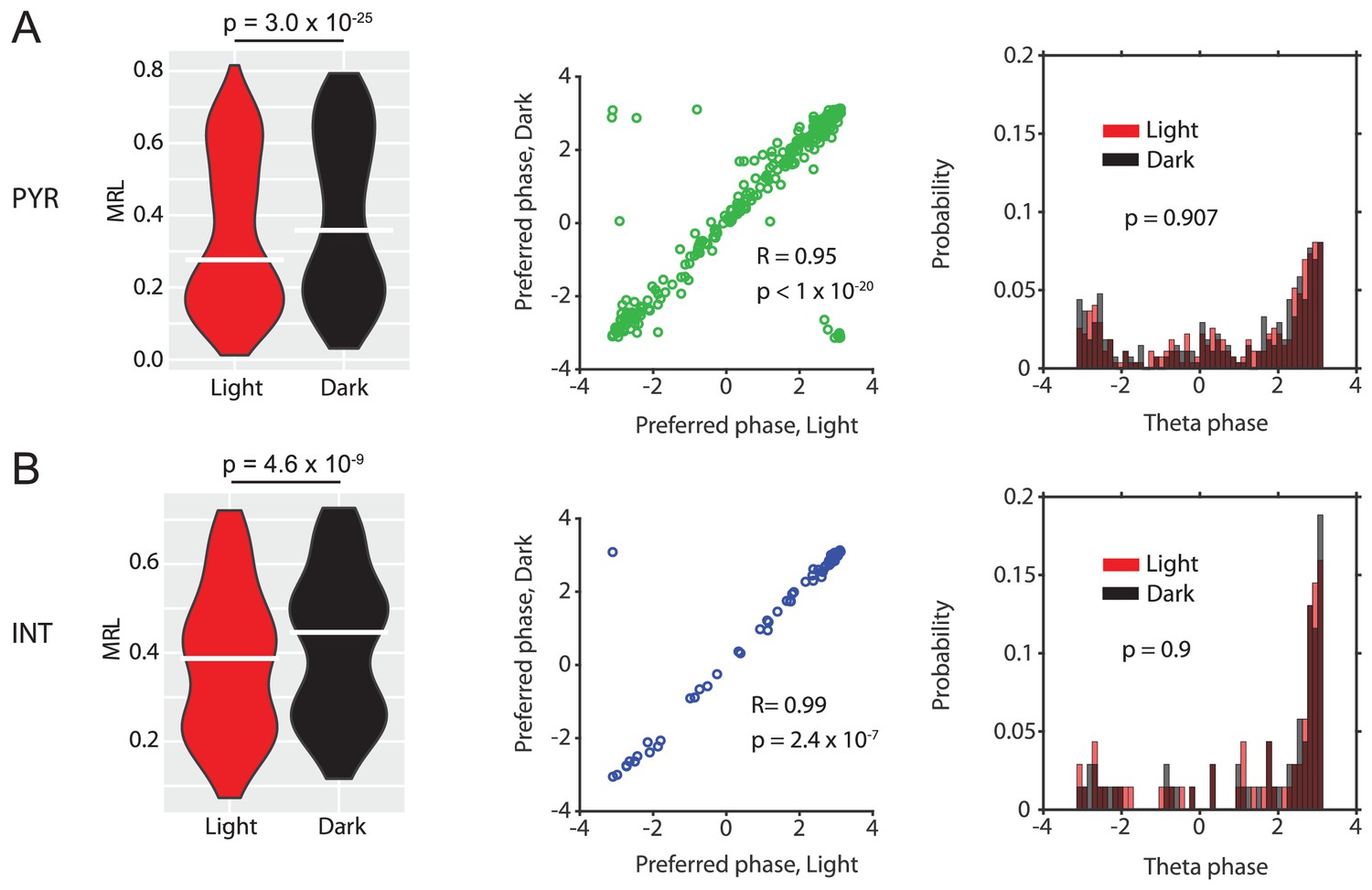
Data for n = 273 putative principal neurons (PN) (A) and n = 69 putative interneurons (IN) (B).
Violin plots show theta-phase locking of theta rhythmic PNs or theta rhythmic INs during light and dark conditions; p-values from Wilcoxon signed-rank test. Scatter plots show preferred LFP theta phases during light and dark for PNs (green) or INs (blue). Note the high circular-linear correlations for PNs and INs. Third panels in A and B show probability-normalized histograms of preferred LFP theta phases during light and dark for PNs and INs. Note that the majority of both PNs and INs preferentially fire around the trough of layer II/III LFP theta oscillations, and a minority preferred firing around the peak. No significant differences were observed between light and dark conditions in PNs or INs; p-values from Kolmogorov-Smirnov test.
Figure 4 with 2 supplements
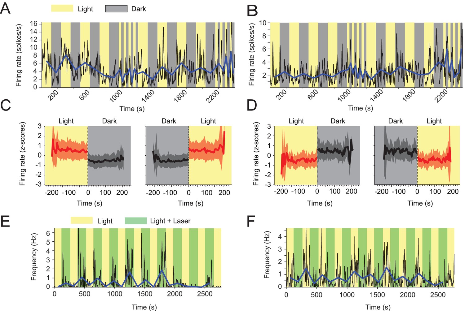
Visual inputs alter mean firing rates of neurons in the medial entorhinal cortex.
(A-D) Yellow and gray backgrounds indicate duration of light and dark epochs, respectively. (A) Data on firing rate from one example neuron in the medial entorhinal cortex (MEC) with its baseline firing rate negatively modulated by darkness. Black lines show the firing rate at 1 s resolution. Blue line connects the mean firing rate in each light or dark epoch. (B) Data on firing rate from one example neuron in the MEC whose baseline firing rate is positively modulated by darkness; same visualization scheme as in A. (C) Left and right panels show the mean z-scored firing rate across n = 139 neurons with significantly negative modulation of firing rates by darkness (see Materials and methods) in 5 s bins around the transition point from light to dark and dark to light, respectively. Red color indicates data from the light condition, black and gray color indicate data from the dark condition. Solid lines and shaded areas show mean and SD. (D) Same as C, but for neurons with positive modulation of baseline firing rates by darkness; n = 32. (E, F) Yellow background indicates light condition, green background indicates the presence of an egocentrically stable spot of green laser light above the animal’s head during the standard light condition. (E) Data on one example neuron in the MEC showing positive modulation of baseline firing rate in presence of the green laser light spot. Same visualization scheme as in A and C. (F) As in E, but for one example neuron with negative modulation of baseline firing rate. Mean firing rates and running speed-adjusted mean firing rates of neurons during light and dark conditions are provided in Figure 4—source data 1.
-
Figure 4—source data 1
Data table of mean firing rates and running speed-adjusted mean firing rates during light and dark conditions of the 171 neurons with significant modulation of firing rates by visual inputs.
- https://cdn.elifesciences.org/articles/62500/elife-62500-fig4-data1-v2.xlsx
Figure 4—figure supplement 1
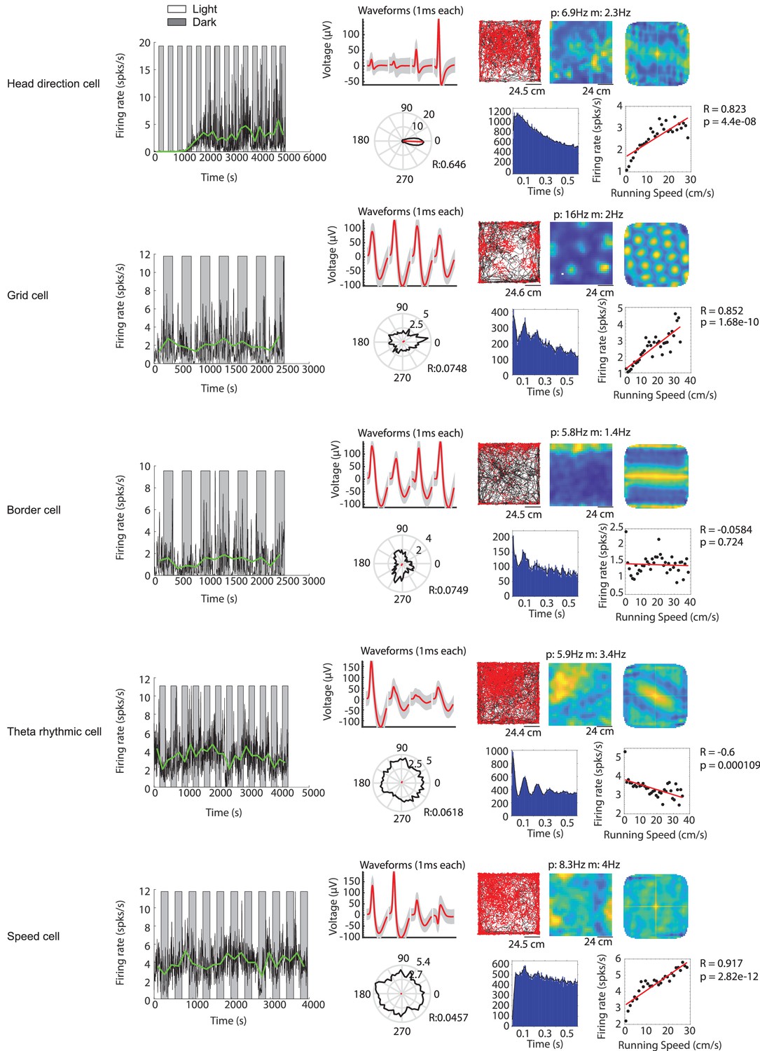
Examples of functional cell types in the medial entorhinal cortex whose baseline firing rates are modulated by visual inputs.
Example cells include (from top to bottom) a head direction cell, a grid cell, a border cell, a theta rhythmic cell and a speed cell. For each functional cell type example: Left most panel shows the firing rate in 1 s time bins (black solid line) and the mean firing rate of each light or dark epoch (green solid line) for one recording session. Gray background indicates the dark condition; white background indicates the light condition. The remaining panels in the top row from left to right show the waveform plot, trajectory plot, firing rate map, and spatial autocorrelation of the firing rate map. The bottom row from left to right shows the head direction map, spike autocorrelogram, and speed tuning plot. In the waveform plot, red solid lines show the mean waveforms of all spikes for the four tetrode channels (each 1 ms long). Gray shading shows the s.e.m. of the waveform across all spikes. In the trajectory plot, black lines show the trajectory of the mouse, and red dots indicate the location of spikes on that trajectory. The firing rate map shows the occupancy-normalized firing rate per spatial bin, blue color indicates low firing rate, yellow color indicates high firing rate; p=peak firing rate; m = mean firing rate. Same color scheme applies for the spatial autocorrelation of the firing rate map. The solid black line in the head direction plot shows the occupancy-normalized firing rate per head direction bin (bin size is 15 degree) on a circular axis; numbers next to the inner and outer circle are the circular axis tick mark labels. The solid red line shows the mean resultant length; R = circular correlation. Black dots in the speed tuning plot show the mean firing rate across all data points for 2 cm/s running speed bins. The red line shows the linear regression. R = Pearson’s correlation coefficient; p=p value for linear regression.
Figure 4—figure supplement 2
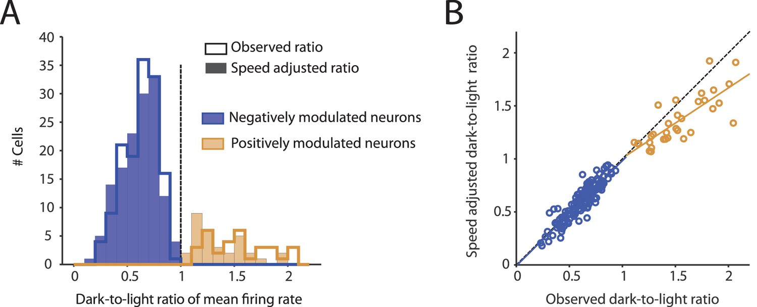
Observed changes in mean firing rates during darkness are not an artifact of changes in running speed.
(A) Histograms show the distribution of dark-to-light ratios of mean firing rates of neurons whose firing rates are negatively (blue, n = 139) and positively (ocher, n = 32) modulated by darkness. The step histograms show the dark-to-light ratios computed from the observed firing rates; the filled histograms show the running speed-adjusted dark-to-light ratios. Before running speed adjustment, mean firing rates of negatively and positively modulated neurons were reduced and increased during darkness to 0.62 ± 0.16 and 1.53 ± 0.28 of the firing rates during the light condition, respectively. After running speed adjustment, these values were 0.61 ± 0.17 (mean adjustment = –0.014, CI = [–0.002 –0.026], t = –2.31, df = 138, p=0.023, t-test) and 1.36 ± 0.23 (mean adjustment = –0.174, CI = [–0.112 –0.235], t = –5.78, df = 31, p=2.3×10⁻⁶), respectively. (B) Scatter plot showing the strong correlations of the observed dark-to-light ratios of changes in mean firing rates with the running speed-adjusted dark-to-light ratios in negatively modulated neurons (blue, n = 139, R = 0.91, p<1×10–20) and positively modulated neurons (ocher, n = 32, R = 0.79, p=7.9×10⁻⁸).
Figure 5 with 2 supplements
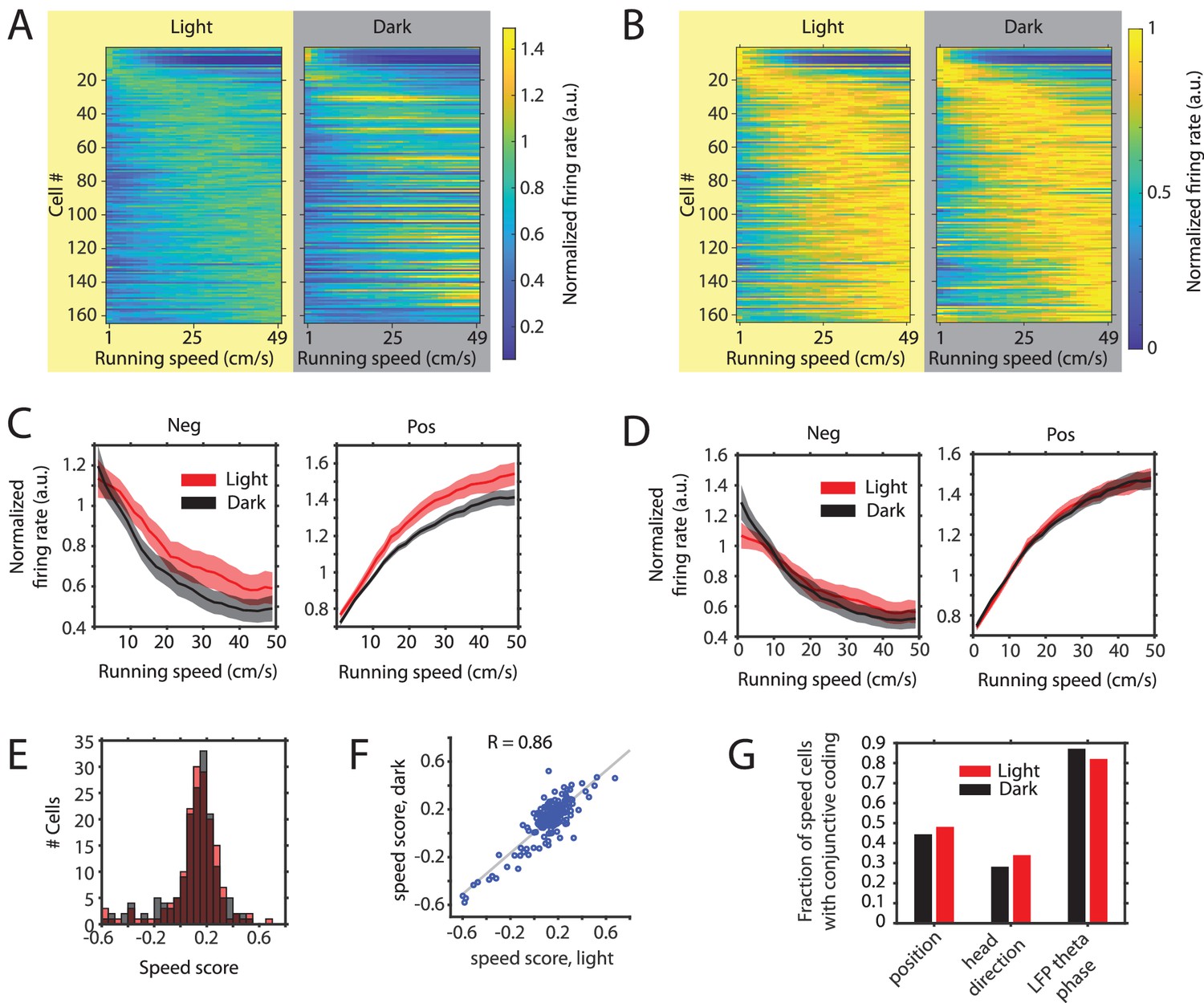
Changes in the slope of speed tuning curves during darkness are largely explained by changes in mean firing rate as opposed to changes in the running speed-dependent gain in firing rates.
(A) Left and right panels show speed response curves for the n = 164 neurons passing statistical significance of speed modulation in the LN-model (see Materials and methods) for either the light or dark condition, respectively. For comparison of speed response curves across neurons and between light and dark conditions, firing rates were normalized across conditions to the maximum in the light condition; Cells were sorted by the location of peak firing on the running speed axis averaged across light and dark conditions and each row in the left and right panels corresponds to the same cell. (B) Same data as in A, but speed response curves were normalized to their maxima within conditions, which allows a comparison of the running speed-dependent gain in firing rates. (C) Left and right panels show speed response curves of negatively (n = 26) and positively (n = 138) modulated neurons after normalization to the mean firing rate across conditions; solid lines and shaded areas show mean ± s.e.m. across neurons, see Table 5 on statistics (D) Left and right panels show speed response curves of negatively (n = 26) and positively (n = 138) modulated neurons after normalization to the mean firing rate within conditions; solid lines and shaded areas show mean ± s.e.m. across neurons; see Table 6 on statistics (E) Histogram of speed scores for all neurons showing significant speed modulation in either the light or dark condition. Red and gray color indicate data on light and dark, respectively. (F) Scatter plot comparing speed scores during the light with speed scores during the dark condition. (G) Percentage of cells showing conjunctive coding of running speed and either position, head direction, or LFP theta phase during the light and dark conditions. Speed response curves of neurons during light and dark conditions are provided in Figure 5—source data 1.
-
Figure 5—source data 1
Speed response curves during light and dark conditions of the 164 neurons showing significant modulation of firing rates by running speed in either light or dark condition.
- https://cdn.elifesciences.org/articles/62500/elife-62500-fig5-data1-v2.xlsx
Figure 5—figure supplement 1
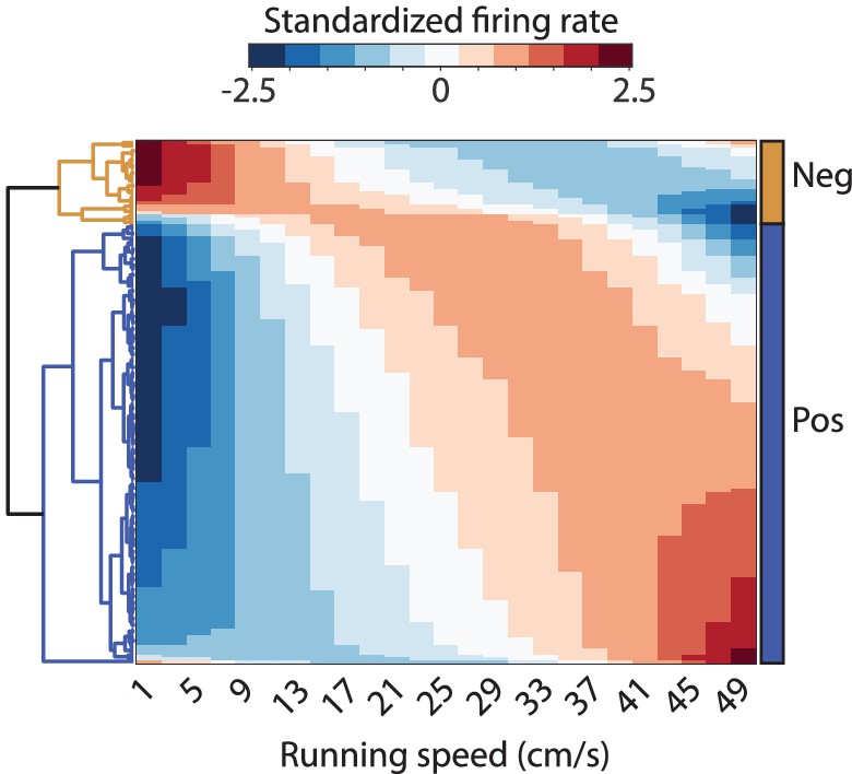
Clustergram visualizing the results of the hierarchical clustering of neurons by similarity of speed modulation of firing rates.
The clustering was performed on the neurons’ average speed response curves across light and dark conditions fitted by a quadratic polynomial.
Figure 5—figure supplement 2
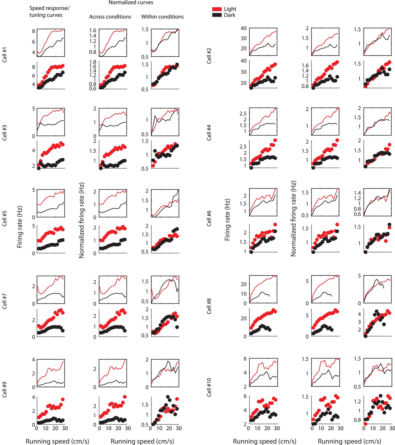
Figure shows the effect of normalizing LN-model derived speed response curves (Hardcastle et al., 2017) and speed tuning curves across or within sessions for ten example cells.
For each example cell, the first row shows the LN-model derived speed response curves and the second row shows the speed tuning curves; the first column shows speed response and tuning curves with absolute firing rate values, the second column shows data after normalization across conditions, and the third column shows data after normalization within conditions. Data for the light condition are shown in red, data for the dark condition are shown in black. Each data point in the speed tuning curve shows the mean over a 2 cm/s speed bin.
Figure 6 with 2 supplements
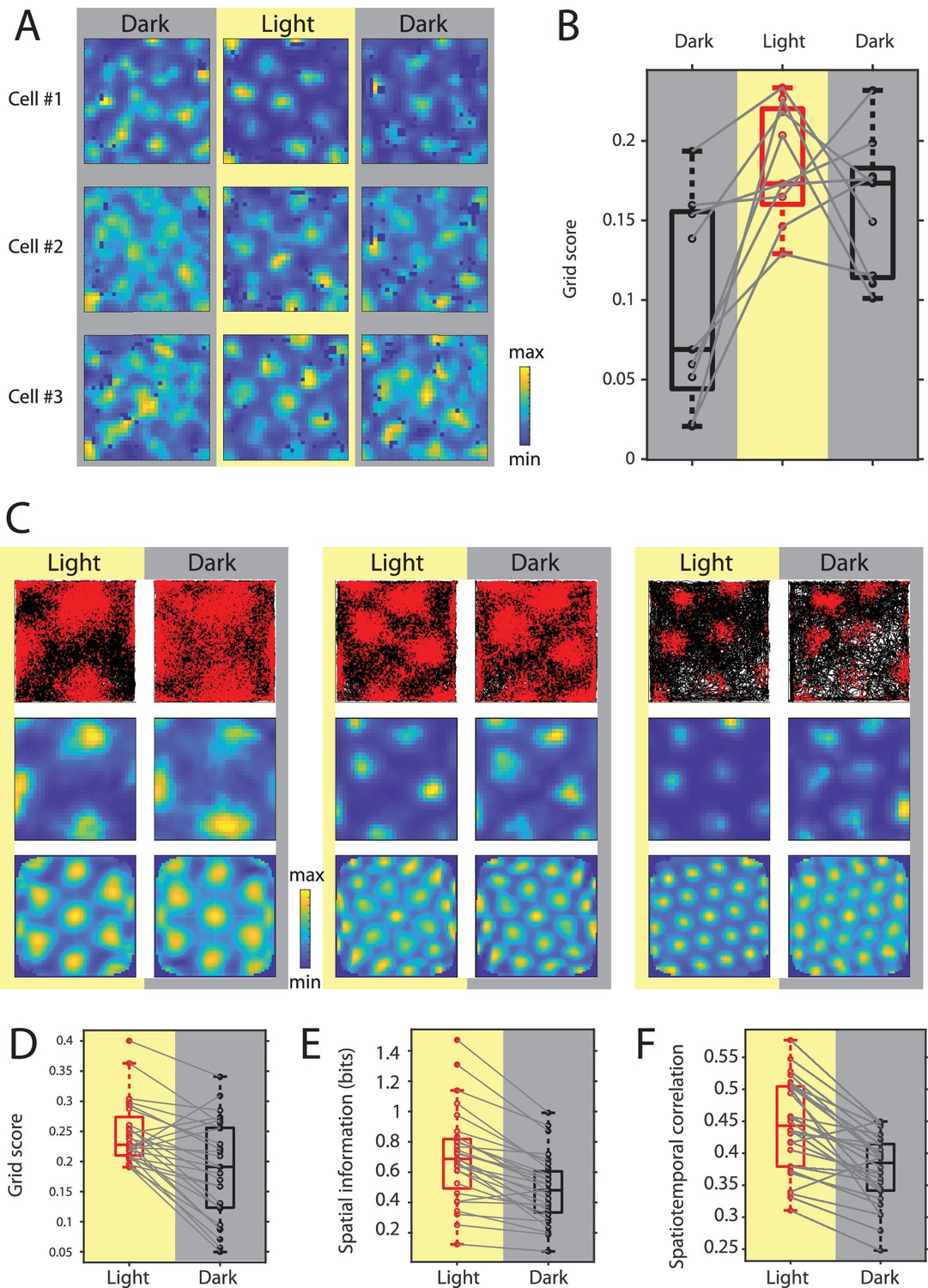
Grid cell spatial firing is maintained but less stable in the absence of visual inputs.
(A) Firing rate maps of three example neurons during sequential dark, light, and dark sessions of 10–20 min duration. In the initial dark session, the animal was introduced to the open-field environment in complete darkness. (B) Box plots of grid scores during sequential dark, light, and dark session, n = 9 neurons from two mice. Black color and gray background indicate data on dark conditions, red color and yellow background indicate data on the light condition. Solid gray lines connect data points from the same grid cell. Chi-square = 10.89, p=0.0043, Friedman’s test; post-hoc tests revealed significant differences between the initial dark and light sessions as well as the initial dark and second dark sessions at alpha = 0.05. (C) Top, middle, and bottom rows show trajectory plots, firing rate maps, and spatial autocorrelations of firing rate maps for three example grid cells recorded over multiple days during alternating light and dark epochs. Solid black lines in the trajectory plot show the trajectory of the animal, red dots mark the location of spikes during that trajectory. (D–F) Box plots of grid scores, spatial information, and spatiotemporal correlation during light and dark; Spatiotemporal correlation is the correlation between the observed firing rate and the expected firing rate computed from the animal’s position in the grid firing rate map during light; gray solid lines connect data points from the same grid cells; p=2.25×10⁻⁴, p=7.26×10⁻⁶, and p=2.79×10⁻⁵; n = 28, Wilcoxon signed-rank test. Firing rate maps of grid cells are provided in Figure 6—source data 1.
-
Figure 6—source data 1
Trajectory plots, firing rate maps, and rate map autocorrelograms of the 28 grid cells analyzed in the current study.
G = grid score; m = mean firing rate across bins of firing rate map; p=peak firing rate in firing rate map.
- https://cdn.elifesciences.org/articles/62500/elife-62500-fig6-data1-v2.pdf
Figure 6—figure supplement 1
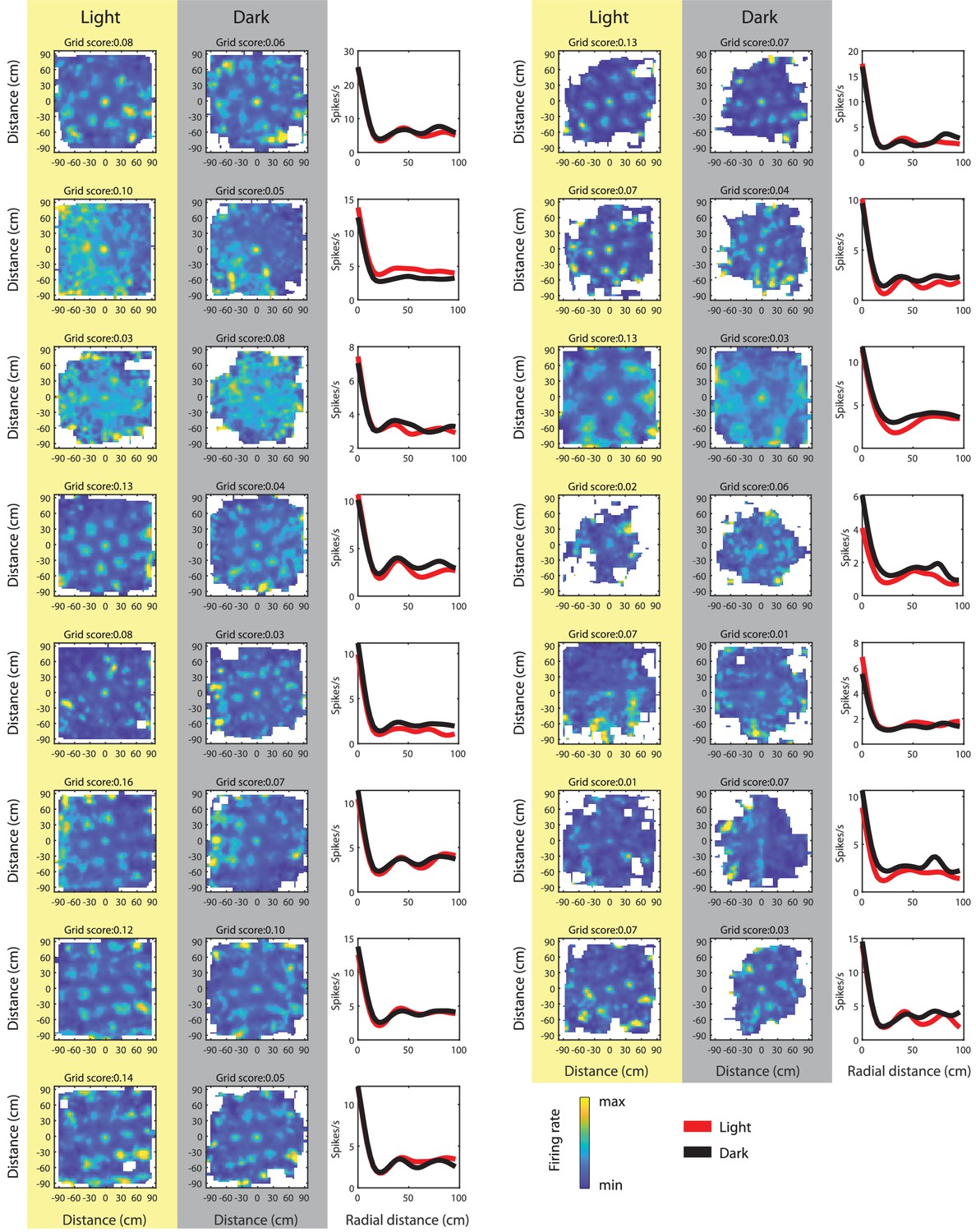
Spike-triggered firing rate maps of grid cells with a grid score >0.06 in either light or dark condition; grid scores computed from the spike-triggered firing rate maps.
Note that grid fields in spike-triggered firing rate maps from the dark condition appear wider, but grid fields have the same spacing, orientation, and phase than during light.
Figure 6—figure supplement 2
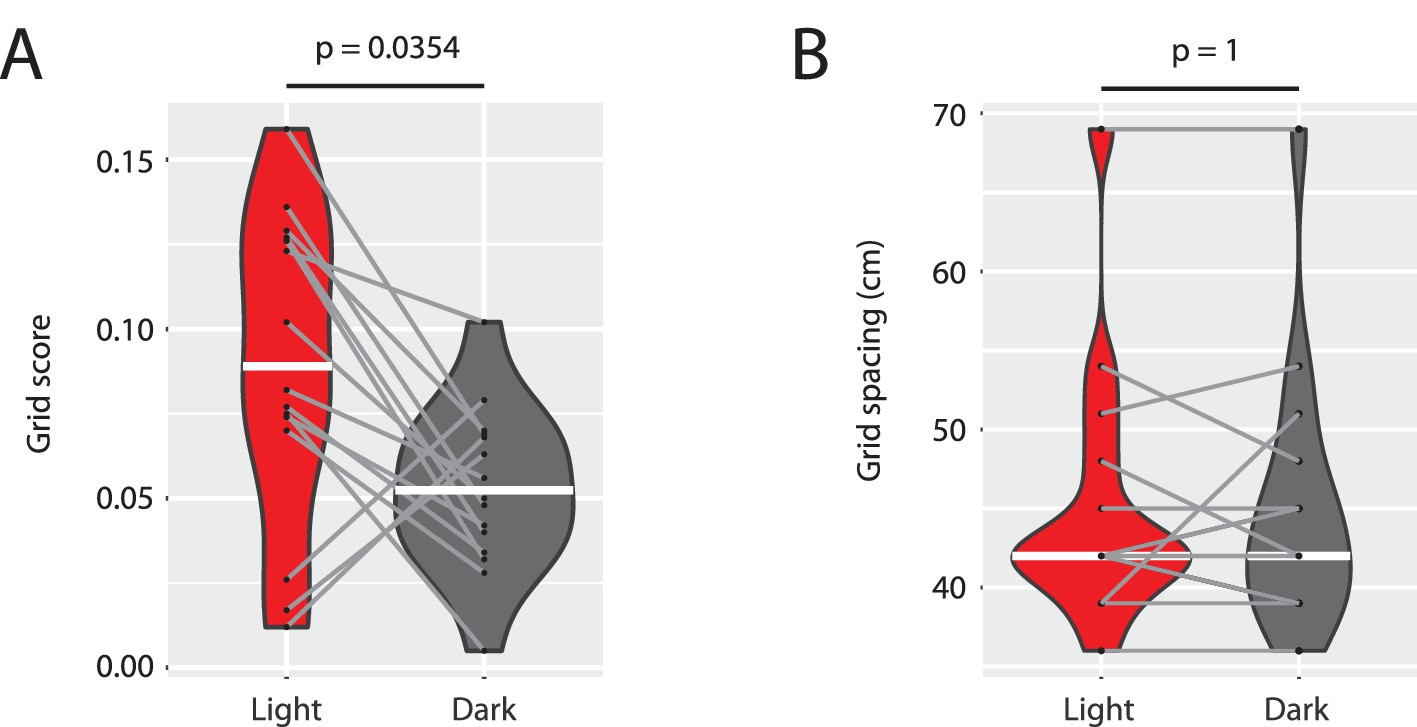
Grid scores are reduced without changes in the spacing of grid maps.
(A) Grid scores computed from spike-triggered firing rate maps from the light and dark condition of the n = 15 grid cells shown in Supplementary Figure 1 related to Figure 6. (B) Grid spacing (first peak location in the radial distance plots shown in Supplementary Figure 1 related to Figure 6) for the same n = 15 grid cells in the light and dark condition. White horizontal lines indicate the median of the distribution. Gray lines connect data from the same cell. p-values from Wilcoxon signed-rank test.
Figure 7 with 2 supplements
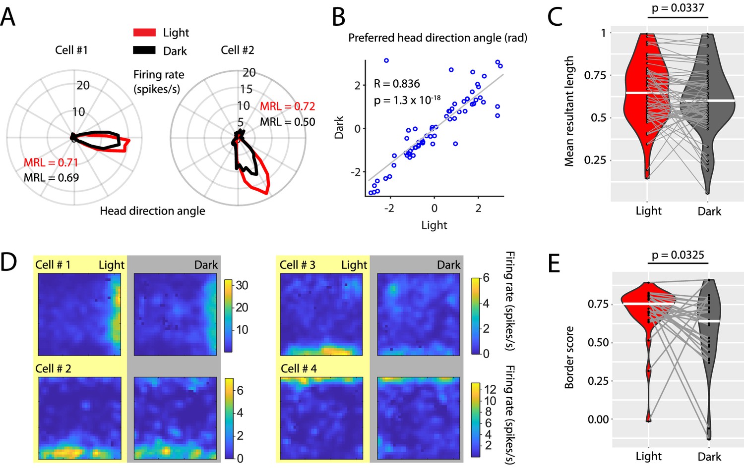
Visual inputs sharpen the tuning curves of head direction cells and border cells.
(A) Polar histograms showing the head directional tuning of two head direction cells during light (red) and dark (black) conditions. (B) Scatter plot comparing the preferred head direction angles of n = 67 head direction cells between light and dark conditions. Note the strong circular-linear correlation. (C) Violin plots showing the distributions of mean resultant lengths of head directional tuning curves for light (red) and dark (gray) conditions. White horizontal lines mark the medians. Gray horizontal lines connect data points from the same neuron. p=0.0377, Wilcoxon signed-rank test. (D) Firing rate maps of four border cells for light and dark conditions. (E) Violin plots comparing the distribution of border scorers of n = 27 border cells between light and dark conditions. p=0.0325, Wilcoxon signed-rank test. Underlying data on mean resultant lengths of head direction tuning during light and dark conditions are provided in Figure 7—source data 1.
-
Figure 7—source data 1
Data on mean resultant lengths of head direction tuning during light and dark conditions for the 67 neurons with significant head direction tuning in either light or dark condition.
- https://cdn.elifesciences.org/articles/62500/elife-62500-fig7-data1-v2.xlsx
Figure 7—figure supplement 1
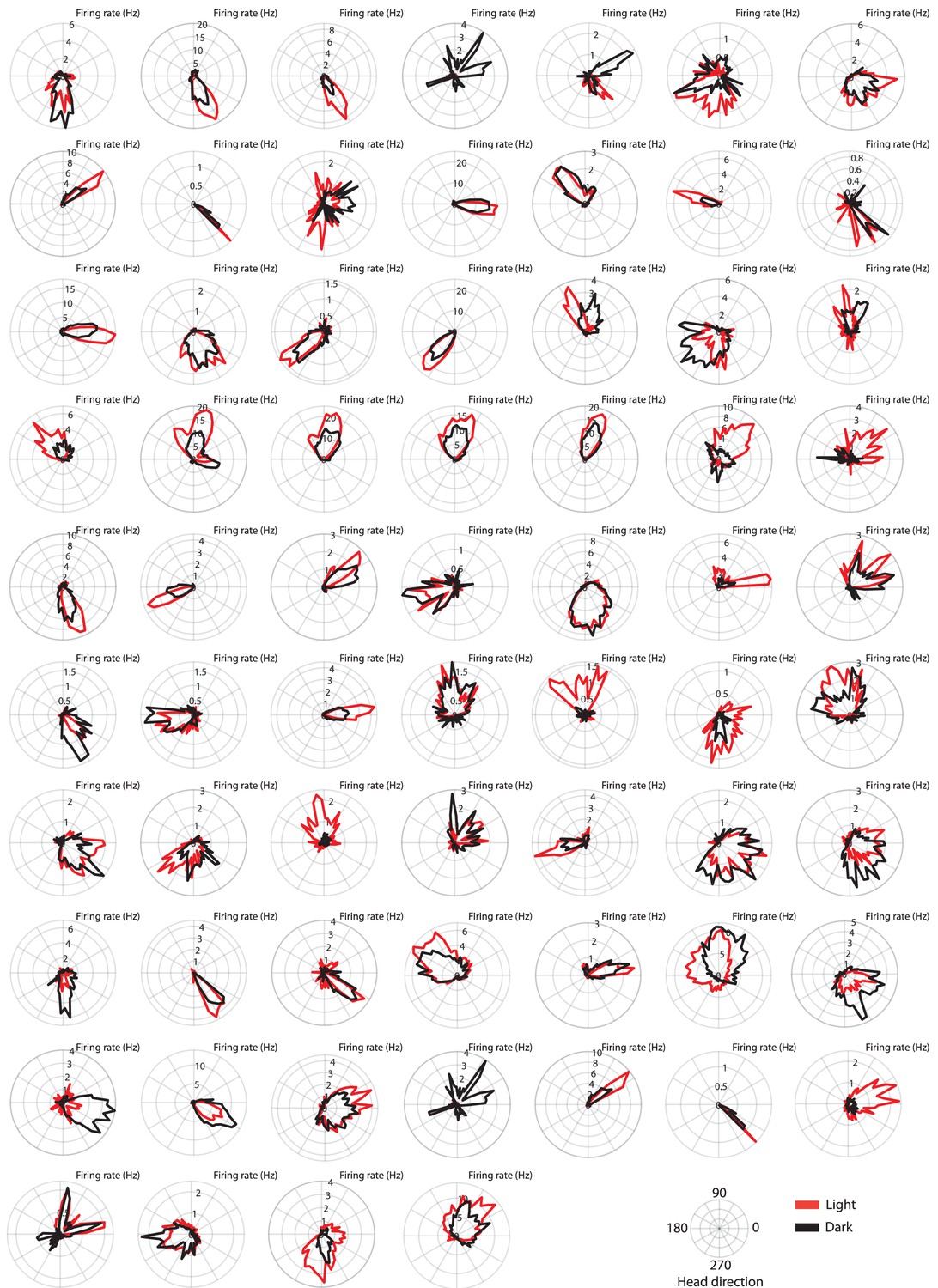
Polar histograms showing the head directional tuning in light and dark conditions of the 69 head direction cells analyzed in this study.
Note that in the dark condition, head direction cells maintain tuning to their preferred head direction angles, but tuning curves become slightly broader. Note also that, in addition to tuning curves becoming broader, mean firing rates are often changed between light and dark conditions.
Figure 7—figure supplement 2
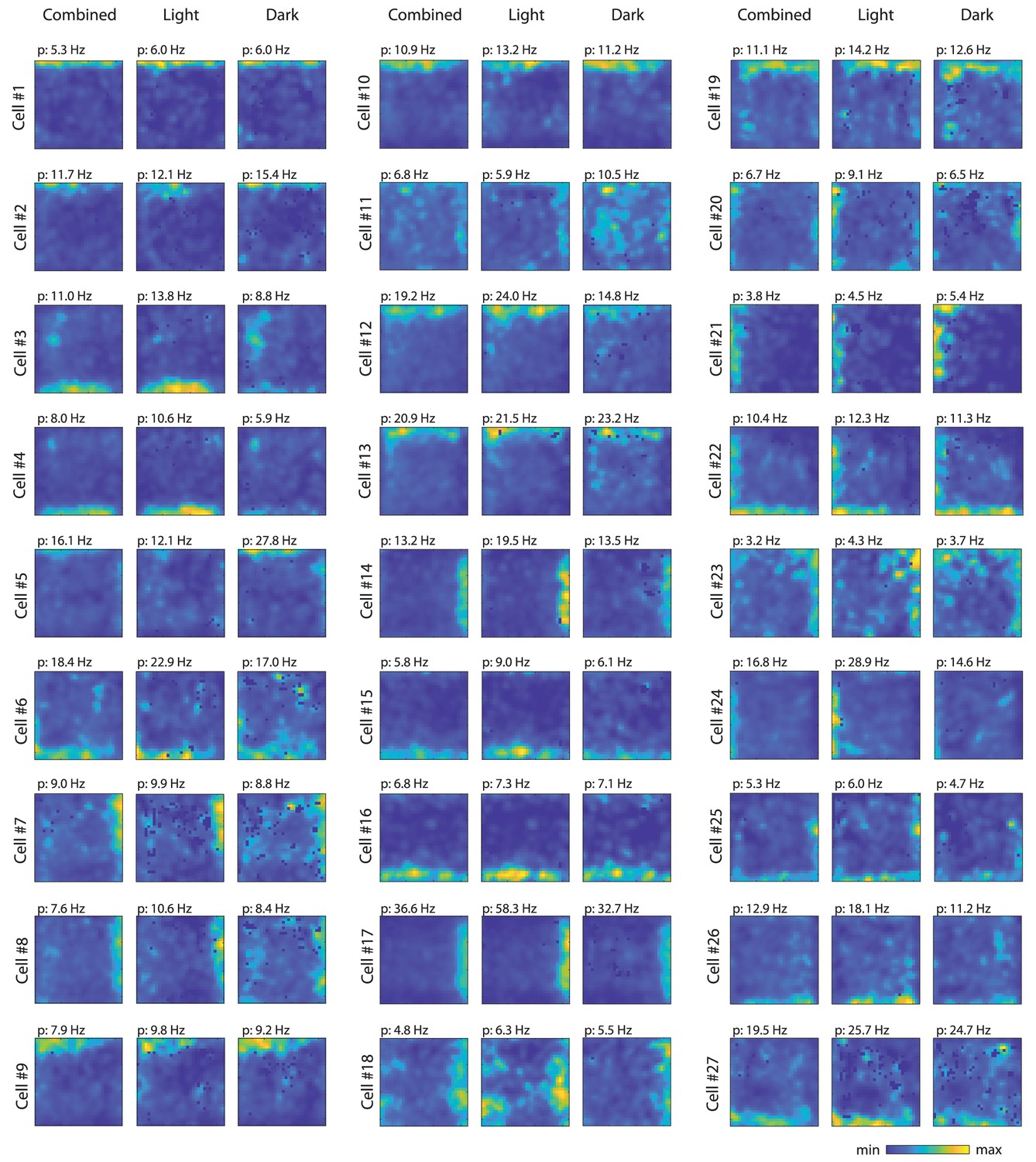
Firing rate maps for the 27 border cells identified in this study.
For each cell, first panel shows the firing rate map from the whole recording session (light and dark epochs combined), second panel shows the firing rate map from the light condition, and third panel shows the firing rate map from the dark condition. For each cell, the same color scale was used across conditions; p=peak firing rate.
Figure 8 with 2 supplements
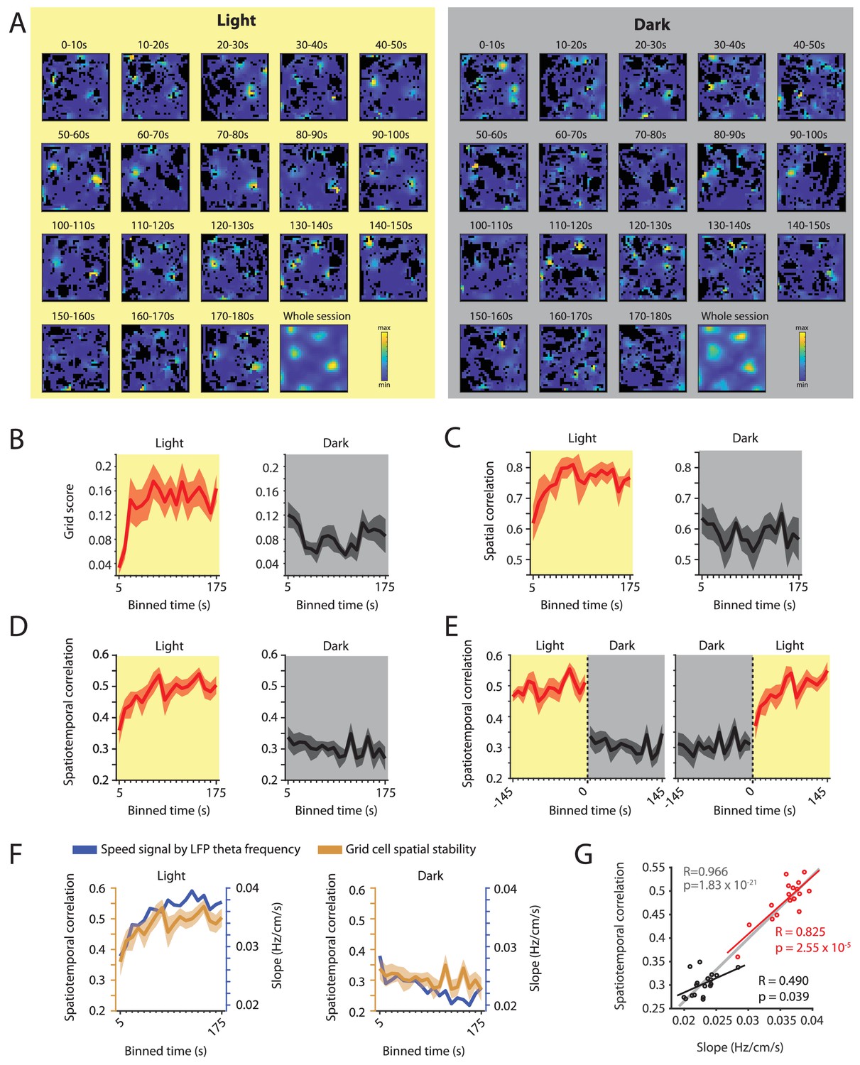
Changes in grid cell spatial stability as a function of time correlate with changes in the slope of the local field potential theta frequency vs. running speed relationship.
(A) Firing rate maps for consecutive 10 s bins of data after transitioning from dark to light (left side, yellow background) and light to dark (right side, gray background) for one example neuron. (B–D) Time course measured in 10 s bins of grid scores (B) spatial correlation (C) and spatiotemporal correlation (D) during the first three minutes of light and dark sessions. Solid lines show mean firing rates, shaded area indicates s.e.m.; n = 7 cells from three mice. (E) Left and right panels show 10 s binned data on spatiotemporal correlation around the transition points from light to dark and dark to light, respectively. (F) Overlay of data shown in D and 1I showing the temporal alignment of changes in the slope of the theta frequency vs. running speed relationship (blue colors) and the spatial stability of grid cell firing measured by the spatiotemporal correlation (ocher colors). Each data point shows the mean values in 10 s time bins of the first 180 s after the start of the light (left panel) or dark (right panel) condition. (G) Scatter plot of time-binned data shown in F; each data point shows the mean values of the slope and grid cell stability at each of the time points shown in F. Red and black lines show the linear regressions of data in the light and dark conditions, respectively (Light: R = 0.825, p=2.55×10⁻⁵, n = 18 time points; Dark: R = 0.490, p=0.039, n = 18 time points). Gray line shows the linear regression of the combined data set, n = 36 (18 time points x two conditions), R = 0.966; p=1.83×10⁻²¹.
Figure 8—figure supplement 1
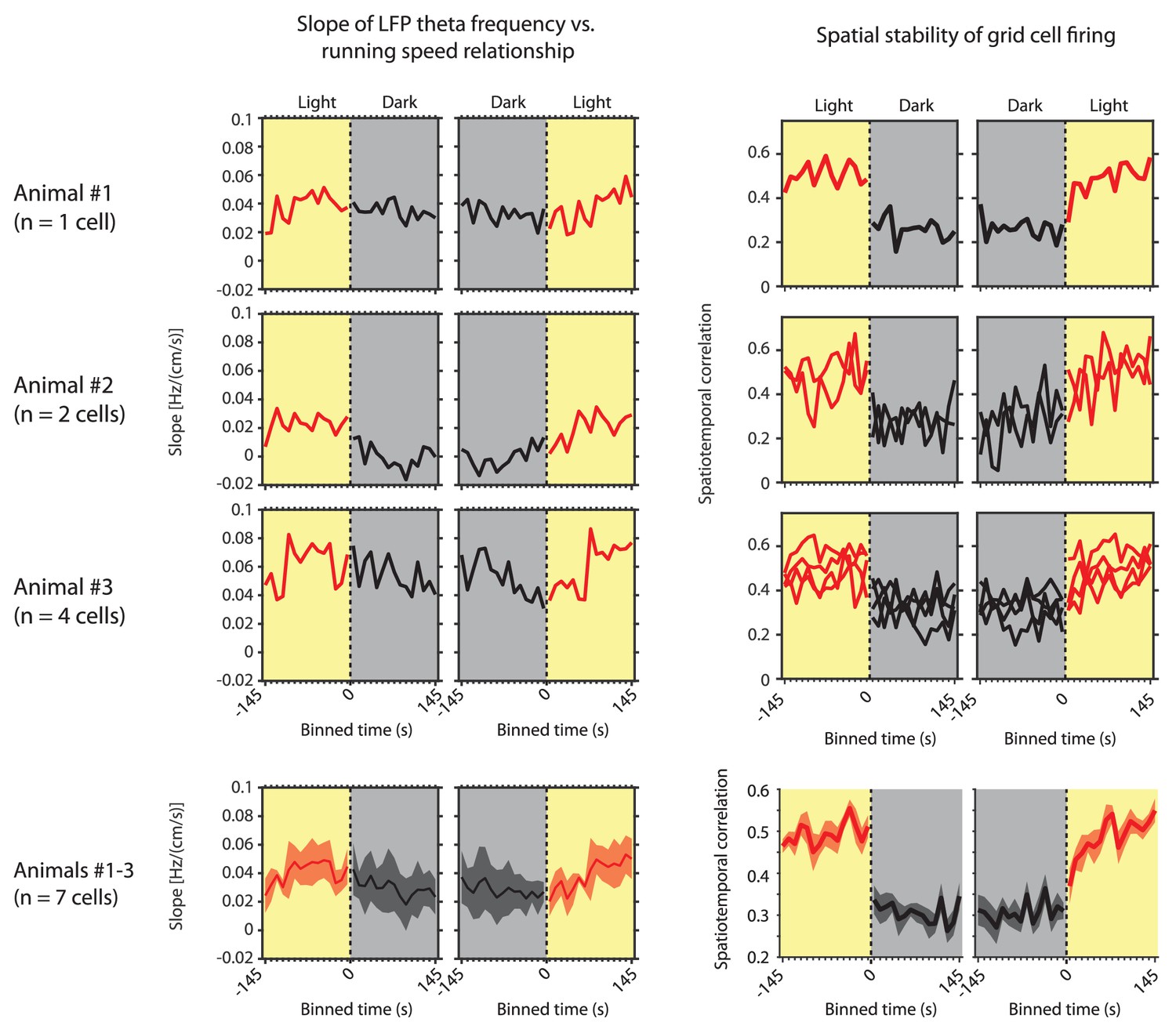
Left side shows the slope of the local field potential (LFP) theta frequency vs. running speed relationship as a function of 10 s time bins around the transition points from light to dark and from dark to light for the three individual mice in which grid cells could be recorded over multiple days and sessions.
Right side shows the corresponding spatial stability of grid cells recorded in each of those mice as a function of 10 s time bins around the transition points from light to dark and from dark to light. The last row shows the same data for slope and grid cell stability as mean ± s.e.m. across mice or cells, respectively.
Figure 8—figure supplement 2

Changes in grid cell spatial stability as a function of time do not align with changes in the y-intercept of the local field potential theta frequency vs. running speed relationship.
(A) Overlay of data shown in Figure 8D and 1J comparing the time course of changes in the y-intercept of the theta frequency vs. running speed relationship (blue colors) and the spatial stability of grid cell firing measured by the spatiotemporal correlation (ocher colors). Left and right panels show data on first three minutes in the light and dark conditions, respectively. (B) Scatter plot of time-binned data shown in A (each data point shows the mean values of y-intercept and grid cell stability at each time point in A). Black line shows the linear regression of data in the dark condition; n = 18 time points, R = 0.056, p=0.83. Red line shows the linear regression in the light condition; n = 18 time points, R = –0.633, p=0.0048.
Tables
Table 1
related to Figure 2.
Statistics on the changes in the frequency of theta rhythmic firing as a function of running speed for principal cells and interneurons during light and dark conditions. Results from a linear mixed effects model. PN = principal neurons, IN = interneurons, SE = standard error, df = degrees of freedom, CI = confidence intervals.
| Estimate | SE | t-statistic | df | p-value | CI | |||
|---|---|---|---|---|---|---|---|---|
| PN | Light | 0.0463 | 0.0126 | 3.69 | 303 | 0.0003 | 0.0216 | 0.0710 |
| Dark | −0.0133 | 0.0091 | −1.47 | 503 | 0.1424 | −0.0312 | 0.0045 | |
| Light−Dark | −0.0597 | 0.0152 | −3.92 | 806 | 0.0001 | −0.0895 | −0.0298 | |
| IN | Light | 0.0583 | 0.0132 | 4.43 | 203 | 1.55E-05 | 0.0324 | 0.0843 |
| Dark | 0.0220 | 0.0124 | 1.77 | 243 | 0.0774 | −0.0024 | 0.0465 | |
| Light−Dark | −0.0363 | 0.0181 | −2.00 | 446 | 0.0461 | −0.0720 | −0.0006 | |
Table 2
related to Figure 2.
Statistics on the changes in the magnitude of theta rhythmic firing as a function of running speed for principal cells and interneurons during light and dark conditions. Results from a linear mixed effects model. PN = principal neurons, IN = interneurons, SE = standard error, df = degrees of freedom, CI = confidence intervals.
| Estimate | SE | t-statistic | df | p-value | CI | |||
|---|---|---|---|---|---|---|---|---|
| PN | Light | 0.0013 | 0.0014 | 0.9084 | 303 | 0.3644 | −0.0015 | 0.0041 |
| Dark | −0.0012 | 0.0008 | −1.46 | 503 | 0.1441 | −0.0027 | 0.0004 | |
| Light−Dark | −0.0025 | 0.0015 | −1.63 | 806 | 0.1036 | −0.0054 | 0.0005 | |
| IN | Light | 0.0079 | 0.0014 | 5.70 | 203 | 4.17E-08 | 0.0051 | 0.0106 |
| Dark | −0.001 | 0.0008 | −0.95 | 243 | 0.3424 | −0.0022 | 0.0008 | |
| Light−Dark | −0.0086 | 0.0015 | −5.69 | 446 | 2.33E-08 | −0.0115 | −0.0056 | |
Table 3
related to Figure 2.
Statistics on the differences in frequency of theta rhythmic firing between putative principal neurons and interneurons. Results from a linear mixed effects model. Values are referenced to putative principal neurons. SE = standard error, df = degrees of freedom, CI = confidence intervals.
| Estimate | SE | t-statistic | df | p-value | CI | |||
|---|---|---|---|---|---|---|---|---|
| Light | y-intercept | −1.34 | 0.36 | −3.73 | 506 | 0.0002 | −2.05 | −0.64 |
| slope | 0.0117 | 0.0169 | 0.69 | 506 | 0.4921 | −0.0216 | 0.0450 | |
| Dark | y-intercept | −0.48 | 0.33 | −1.46 | 746 | 0.1454 | −1.12 | 0.17 |
| slope | 0.0327 | 0.0142 | 2.31 | 746 | 0.0212 | 0.0049 | 0.0605 | |
Table 4
related to Figure 2.
Statistics on differences in magnitude of theta rhythmic firing between putative principal neurons and interneurons. Results from a linear mixed effects model. Values are referenced to putative principal neurons. SE = standard error, df = degrees of freedom, CI = confidence intervals.
| Estimate | SE | t-statistic | df | p-value | CI | |||
|---|---|---|---|---|---|---|---|---|
| Light | y-intercept | −0.20 | 0.05 | −4.23 | 506 | 2.8E-05 | −0.30 | −0.11 |
| slope | 0.0060 | 0.0019 | 3.17 | 506 | 0.0016 | 0.0023 | 0.0097 | |
| Dark | y-intercept | −0.1903 | 0.0472 | −4.03 | 746 | 6.10E-05 | −0.28 | −0.10 |
| slope | 0.0004 | 0.0011 | 0.36 | 746 | 0.7163 | −0.0018 | 0.0026 | |
Table 5
related to Figure 5.
Statistics on the differences in speed response curves of positively and negatively speed-modulated neurons between light and dark conditions after normalization across conditions. Results from a linear mixed effects model with the light condition as reference. Pos = positively modulated, Neg = negatively modulated, SE = standard error, df = degrees of freedom, CI = confidence intervals.
| Estimate | SE | t-statistic | df | p-value | CI | |||
|---|---|---|---|---|---|---|---|---|
| Pos | y-intercept | −0.0527 | 0.017571 | −2.99941 | 6896 | 0.0027 | −0.08715 | −0.01826 |
| slope | −0.00176 | 0.000609 | −2.89551 | 6896 | 0.0038 | −0.00296 | −0.00057 | |
| Neg | y-intercept | −0.06784 | 0.025989 | −2.61042 | 1296 | 0.0091 | −0.11883 | −0.01686 |
| slope | −0.00149 | 0.0009 | −1.65711 | 1296 | 0.0977 | −0.00326 | 0.000274 | |
Table 6
related to Figure 5.
Statistics on the differences in speed response curves of positively and negatively speed-modulated neurons between light and dark conditions after correcting for changes in mean firing rates by normalization within conditions. Results from a linear mixed effects model with the light condition as reference. Pos = positively modulated, Neg = negatively modulated, SE = standard error, df = degrees of freedom, CI = confidence intervals.
| Estimate | SE | t-statistic | df | p-value | CI | |||
|---|---|---|---|---|---|---|---|---|
| Pos | y-intercept | 4.10E-05 | 0.012502 | 0.003278 | 6896 | 0.9974 | −0.02447 | 0.024548 |
| slope | −0.00023 | 0.000433 | −0.52947 | 6896 | 0.5965 | −0.00108 | 0.00062 | |
| Neg | y-intercept | 0.067964 | 0.025506 | 2.66459 | 1296 | 0.0078 | 0.017926 | 0.118002 |
| slope | −0.00349 | 0.000884 | −3.95082 | 1296 | 8.21E-05 | −0.00523 | −0.00176 | |
Additional files
Download links
A two-part list of links to download the article, or parts of the article, in various formats.
Downloads (link to download the article as PDF)
Open citations (links to open the citations from this article in various online reference manager services)
Cite this article (links to download the citations from this article in formats compatible with various reference manager tools)
Effects of visual inputs on neural dynamics for coding of location and running speed in medial entorhinal cortex
eLife 9:e62500.
https://doi.org/10.7554/eLife.62500


