Emergence of behaviour in a self-organized living matter network
- Department of Physics & Astronomy, University of Pennsylvania, United States
- Max Planck Institute for Dynamics and Self-Organization, Germany
- Physik-Department and Center for Protein Assemblies, Technische Universität München, Germany
Figures
Figure 1 with 3 supplements

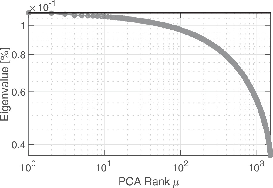
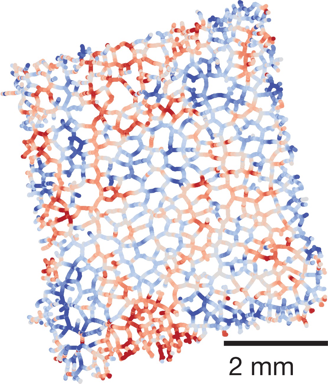
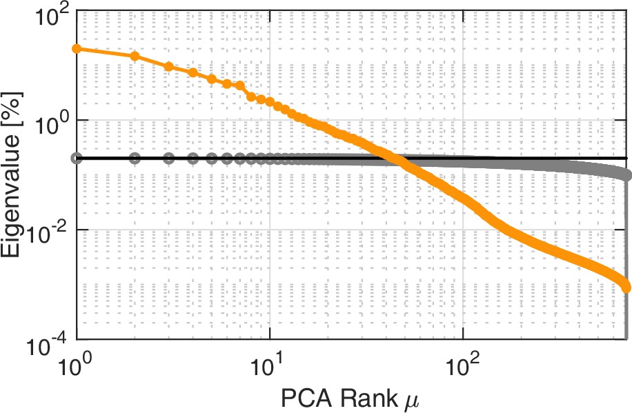
Principal Component Analysis yields a continuous spectrum of contraction modes in the P. polycephalum network.
(A) Example stack of bright-field images of the recorded network. Pixel intensities encode the contraction state (tube dilation) at each point of the network. Principal Component Analysis is performed on a stack of post-processed bright-field frames. (B) Ranked spectrum of relative eigenvalues in percent (orange), plotted against the mode rank on a log-log graph. The eigenvalue spectrum is continuous, without a natural cutoff. Spectrum of randomised data (gray) shown for comparison. The cutoff for the continuous spectrum is defined by the largest eigenvalue of the spectrum from randomised data (black line). (C) (i) Structure of the four highest-ranking modes with their respective coefficients shown in (ii). The red-blue colour spectrum indicates the contraction state. The modes are eigenvectors of the covariance matrix. The coefficient of the first mode captures the organism’s characteristic oscillation period of , while the coefficients show considerable variation in amplitude and frequency over time. The PCA was performed on a data segment with 1500 frames, at the rate of 3 sec per frame.
Figure 1—figure supplement 1
Eigenvalue spectrum computed from randomised data.
Eigenvalue spectrum computed from randomised data.
Figure 1—figure supplement 2
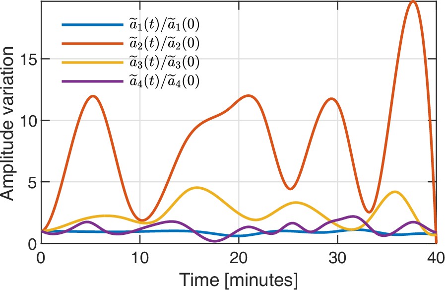
Mode amplitude dynamics over time.
Variation in amplitude of the coefficients of the four top ranked modes over time.
Figure 1—figure supplement 3
Spatial structure of mode .
Contraction mode obtained from Principal Component Analysis of the large rectangular network.
Figure 2
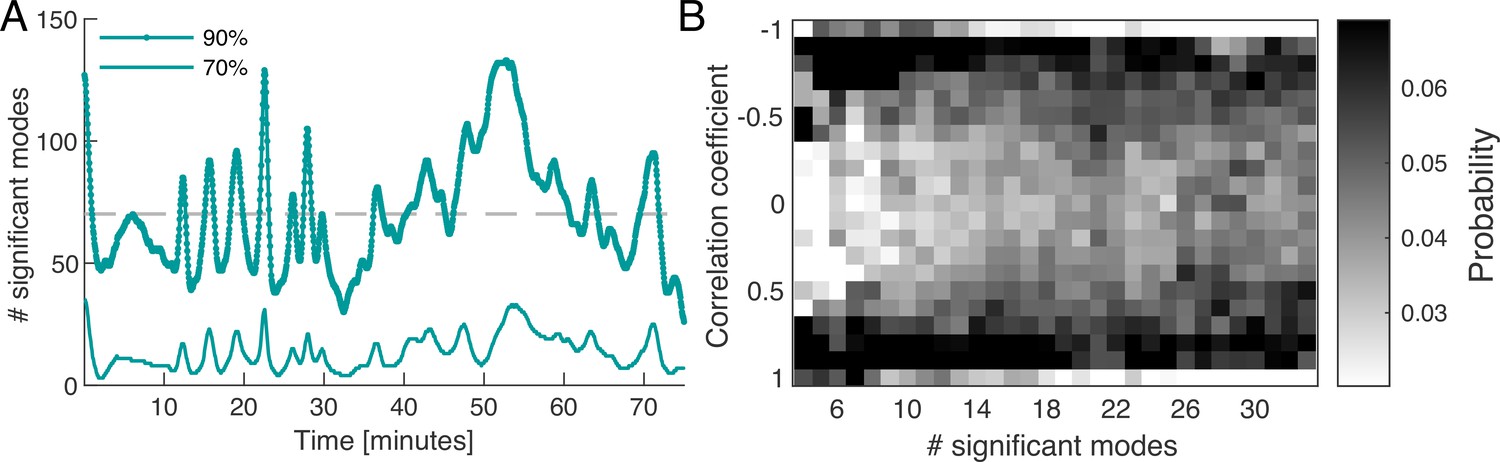
Dynamics of network contraction pattern is subject to strong variability in the percentage of significant modes and correlations between them.
(A) Significant modes given the number of modes required for the cumulative sum of their relative amplitudes to reach 70% (thin light green) and 90% (thick dark green) of the total amplitude plotted over time. Gray dashed line is the mean value of significant modes ( modes or equivalently 4.68% of the total 1500 modes). (B) Distribution of temporal correlation values between mode coefficients depending on the number of significant modes taken from the 70%-cutoff curve in (A). Correlation values show a trend from strong (anti-)correlation for a small number of significant modes (left) to a more uniform distribution of correlation values for a large number of significant modes (right).
Figure 3 with 4 supplements

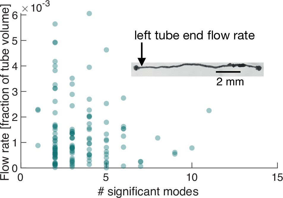
Network growth response to an external attractive stimulus is linked to characteristic changes in the contraction dynamics.
(A) Sequence of bright-field frames showing the network’s growth response to a food stimulus (red arrow in the 84 min). (B) Growth curves of the two most active growth regions of the network. The two tracked regions are indicated by the green and burgundy boxes in the frame at 81 min shown in (A). The growth is shown as the percentage change in area with respect to the initial state at 75 min. After stimulus application, the upper part of the network undergoes significant growth at the expense of the fan-like shaped locomotion front in the lower left corner. (C) The spatial contraction pattern of the three top-ranked modes , , and . (D) Activity of the three top-ranked modes measured by their respective relative amplitude, . After the stimulus (dashed line at 83.5 min), time intervals with a single contraction mode dominating in amplitude (red for the relative amplitude of mode , blue for and yellow for ) prevail over all other modes. Mode amplitudes four to seven are shown in gray for reference. This growth response is paired with activation of mode , as indicated by the pink shaded box extending across (B) and (D). (E) Significant number of modes for a cumulatively summed amplitude of 70% (thin light green) and 90% (thick dark green), over time. Gray dashed line indicates the 6.06% ( modes) average of significant modes for the 90% criterion. When contractions switch from one dominant mode to another, we find time intervals where a larger number of modes have a similar relative amplitude. These times are indicated by the blue shaded boxes extending across (D) and (E).
Figure 3—figure supplement 1
Continuous eigenvalue spectrum compared to randomised spectrum.
Principal Component Analysis yields a continuous spectrum (yellow) of contraction modes in the P. polycephalum network exposed to a food stimulus. The eigenvalue spectrum is computed from data consisting of 700 frames. For comparison we show the eigenvalue spectrum computed from randomised data (gray). The black line indicates the cutoff chosen for the continuous eigenvalue spectrum from the largest eigenvalue of the randomised spectrum.
Figure 3—figure supplement 2
Pre-stimulus link between growth behaviour and contraction patterns.
(A) Bright-field frames showing the network’s growth behaviour pre-stimulus. (B) The spatial contraction pattern of the three top-ranked modes , and . (C) Growth curve of the fan-like locomotion front extending from the bottom left corner of the network. The tracked region is indicated by the green box in the frame at shown in (A). The growth is shown as the percentage change in area with respect to the initial state at . The area of fan-like shaped locomotion front shows strong growth between - followed by stagnation. Subsequently there are two small growth bursts around and . This growth behaviour is paired with activation of mode (red curve), as indicated by the pink shaded boxes extending across (C) and (D). (D) Activity of the three top-ranked modes measured by their respective relative amplitude, . Over long periods of time mode (red curve) is the most dominant mode. Mode amplitudes four to seven are also shown in gray for reference.
Figure 3—figure supplement 3
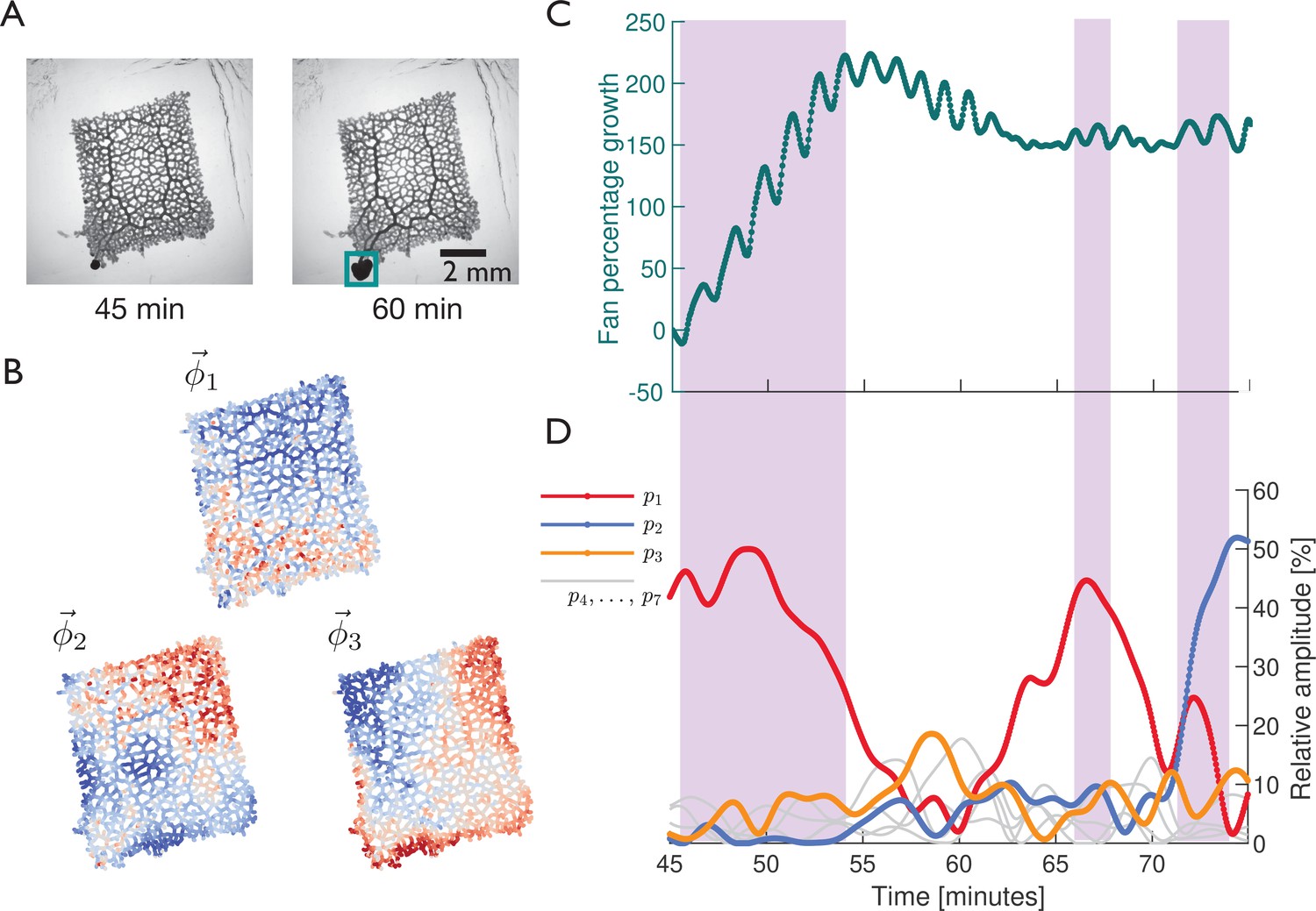
Temporal dynamics of the coefficients of the three top-ranked contraction modes.
Temporal dynamics of the coefficients of the three top-ranked contraction modes (red), (blue) and (yellow) in the large rectangular network. The variation in amplitude, frequency and relative phase shift between coefficients is captured before and after application of the stimulus to the network. The time of stimulus application is indicated by the dashed line.
Figure 3—figure supplement 4

Temporal dynamics of instantaneous mode rank in a pre-stimulus part of the data.
Instantaneous rank of modes over time for the unstimulated network. The top 80 modes are color-coded according to their rank in the eigenvalue spectrum of the same data section used in Figure 3—figure supplement 2. Here we only show a time interval of 10 min. The instantaneous rank is a measure for the activity of a mode and is based on the ranking of relative amplitudes at any given time (see Equation 2). We observe that modes frequently change their instantaneous rank, moving across a wide range of ranks which is only possible in a continuous spectrum.
Figure 4 with 1 supplement
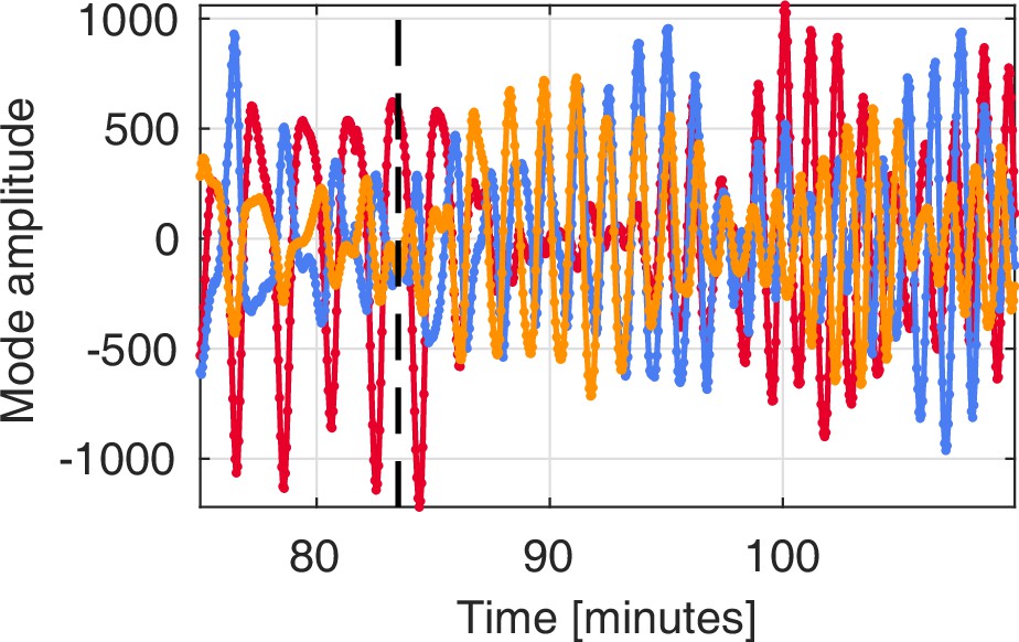
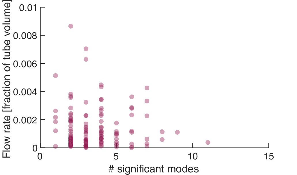
Number of significant modes is indicative for the volume flow rate in a cell reduced in its network complexity to a single tube.
Inset: Single tube with locomotion fronts at both ends. Main plot: Volume flow rate at the left tube end, calculated from tube contraction dynamics versus the number of significant modes at different times. High flow rates are only achieved for a small number of significant modes.
Figure 4—figure supplement 1
Flow rate at the right end of the tube.
Number of significant modes is indicative for the volume flow rate in a cell reduced in its network complexity to a single tube. Volume flow rate at the right tube end, calculated from tube contraction dynamics versus the number of significant modes at different times. High flow rates are only achieved for a small number of significant modes.
Figure 5 with 3 supplements
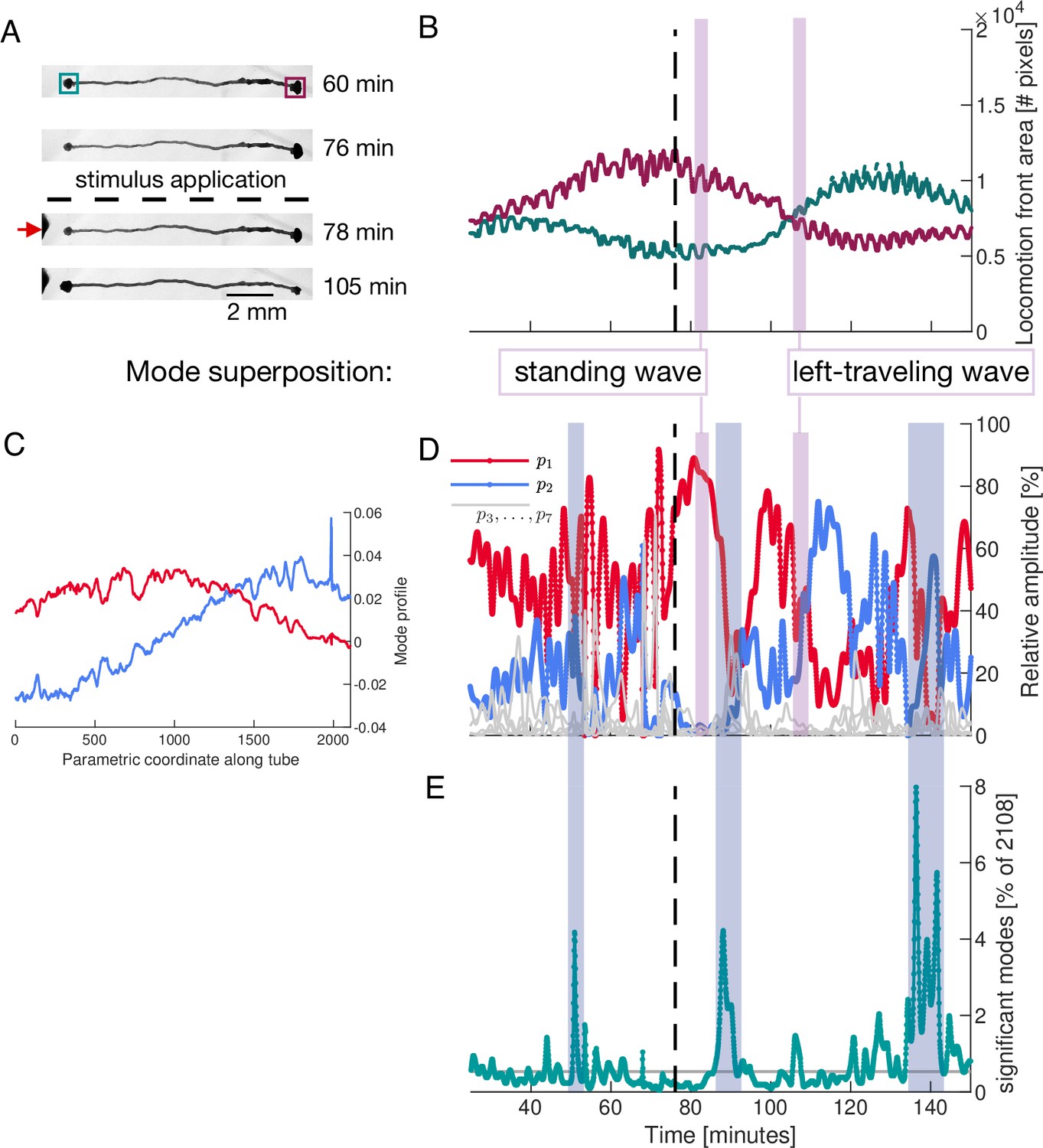
Locomotion behaviour of a single tube is determined by activation and temporal coupling of sine-and cosine-shaped contraction modes.
(A) Sequence of bright-field images showing the locomotion behaviour of the single tube including its response to stimulus application at the left end (red arrow) at 77 min (dashed line). (B) Behaviour of the locomotion front at each end of the tube over time. Tracked regions of the tube are indicated by the green and burgundy boxes in top bright-field frame in (A). (C) Spatial profile of the top-ranked modes and approximately showing sine and cosine shape, respectively. Larger version of the plot is shown in Figure 5—figure supplement 2. (D) Activation of the two top-ranked modes given by their relative amplitude (red and blue). Relative amplitudes of lower ranked modes are shown in gray for comparison. Vertical pink boxes extending across (B) and (D) indicate two representative time intervals and the nature of the two-mode superposition is specified. (E) The number of significant modes over time with 90% cumulative relative amplitude cutoff. Blue boxes extending across (D) and (E) highlight the most pronounced many-mode states.
Figure 5—figure supplement 1
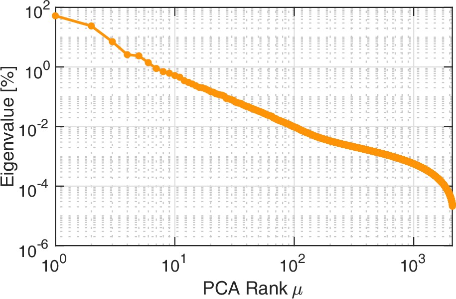
Continuous eigenvalue spectrum.
Principal Component Analysis yields a continuous spectrum of contraction modes in a P. polycephalum specimen with single tube morphology. The eigenvalue spectrum is computed from a data segment which 3300 frames long, including the application of a stimulus to one end of the tube.
Figure 5—figure supplement 2
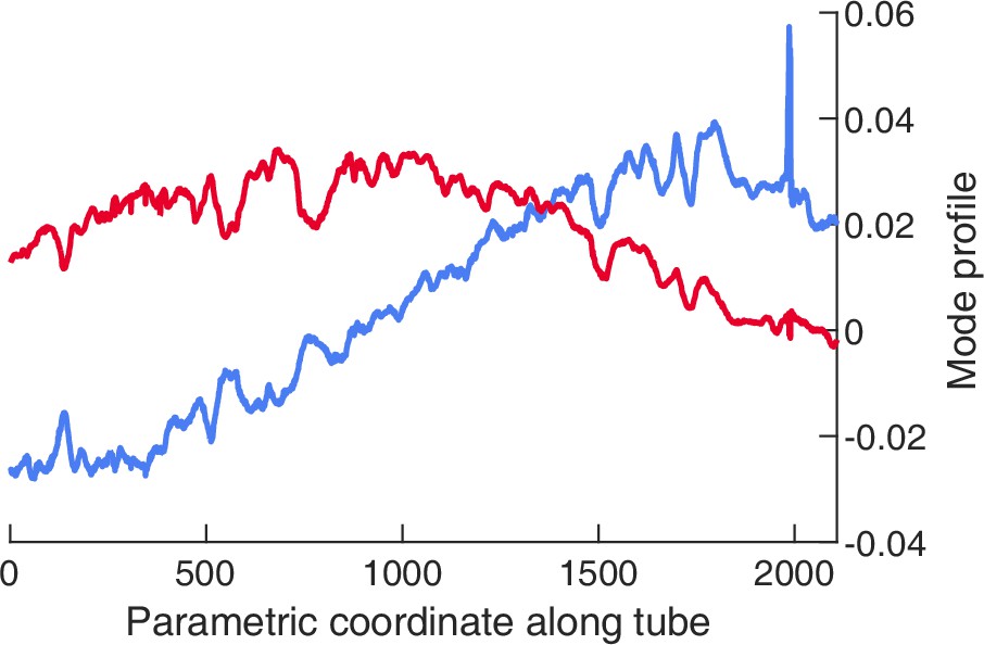
Profile of contraction modes along the single tube.
Top-ranked mode (red) has the shape of a sine function and the second-ranked mode (blue) has cosine shape.
Figure 5—figure supplement 3
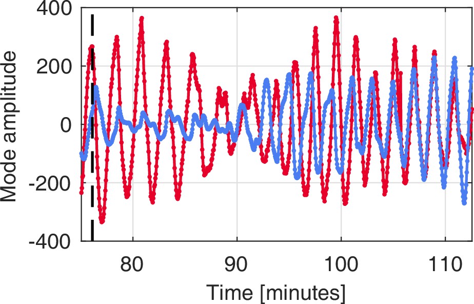
Temporal dynamics of the coefficients of the two top-ranked contraction modes (red) and (blue) in the single-tube P. polycephalum network.
The variation in amplitude, frequency and relative phase shift between coefficients is captured shortly before and after application of the stimulus to the single tube. The time of stimulus application is indicated by the dashed line.
Author response image 1
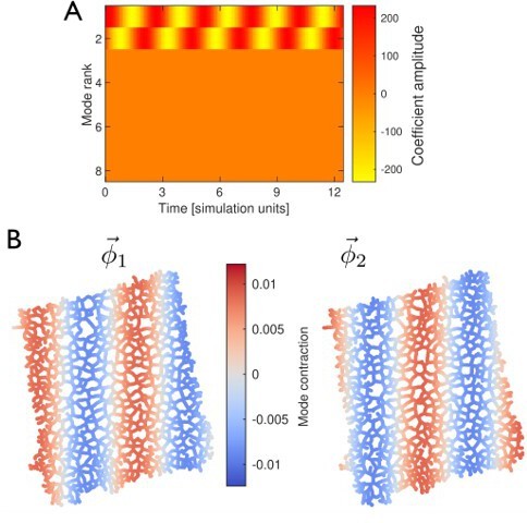
PCA of traveling wave simulated data imposed on the network from the experiment.
Peristaltic wave runs horizontally from right to left across the network. The pattern is fully reconstructed with two PCA modes. (A) The temporal dynamics of the mode coefficients, given by two sine waves shifted by ninety degrees with respect to each other. (B) Spatial structure of the two modes. The spatial patterns are also shifted by a quarter wavelength with respect to each other.
Author response image 2

Dynamics of the number of significant modes in the network (A) and single tube (B) before application of the stimulus.
Dashed line is the mean of the curve. Common to both systems is the large variability in the number of significant modes.
Videos
Video 1
Raw bright field time series of a P. polycephalum network, recorded at a rate of one frame every 3 sec.
Video 2
Raw bright field time series of a single P. polycephalum tube, recorded at a rate of one frame every 3 sec.
Additional files
Download links
A two-part list of links to download the article, or parts of the article, in various formats.
Downloads (link to download the article as PDF)
Open citations (links to open the citations from this article in various online reference manager services)
Cite this article (links to download the citations from this article in formats compatible with various reference manager tools)
Emergence of behaviour in a self-organized living matter network
eLife 11:e62863.
https://doi.org/10.7554/eLife.62863


