Antagonism between killer yeast strains as an experimental model for biological nucleation dynamics
- School of Civil and Environmental Engineering, Cornell University, United States
- Department of Physics, Harvard University, United States
- Department of Molecular and Cellular Biology, Harvard University, United States
- John A Paulson School of Engineering and Applied Sciences, Harvard University, United States
Figures
Figure 1
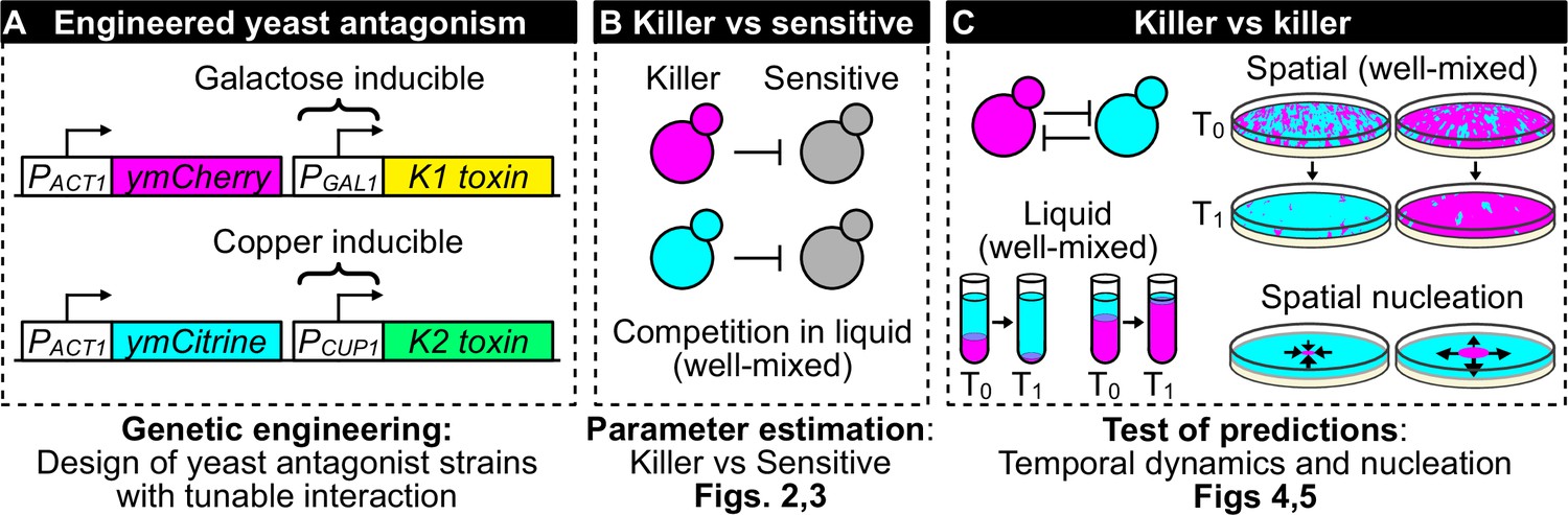
Overview of genetic engineering and experiments performed to investigate the population dynamics of microbial antagonism.
(A) We genetically engineered yeast strains to express two different fluorescent proteins (ymCherry and ymCitrine) constitutively and two different toxin/immunity genes (K1 and K2) in response to the inducers galactose (via the PGAL1 promoter) and copper (via the PCUP1 promoter). (B) We used competition assays between toxin-producing cells (‘killer cells’ in cyan and magenta) and sensitive, nonkiller cells (gray cells) to parametrize mathematical models of toxin production, cell growth, and toxin-induced cell death. (C) We used the models and the experimental system to investigate population dynamics in the presence of antagonistic interactions in both well-mixed (in liquid and on surfaces) and spatially structured populations on surfaces.
Figure 2
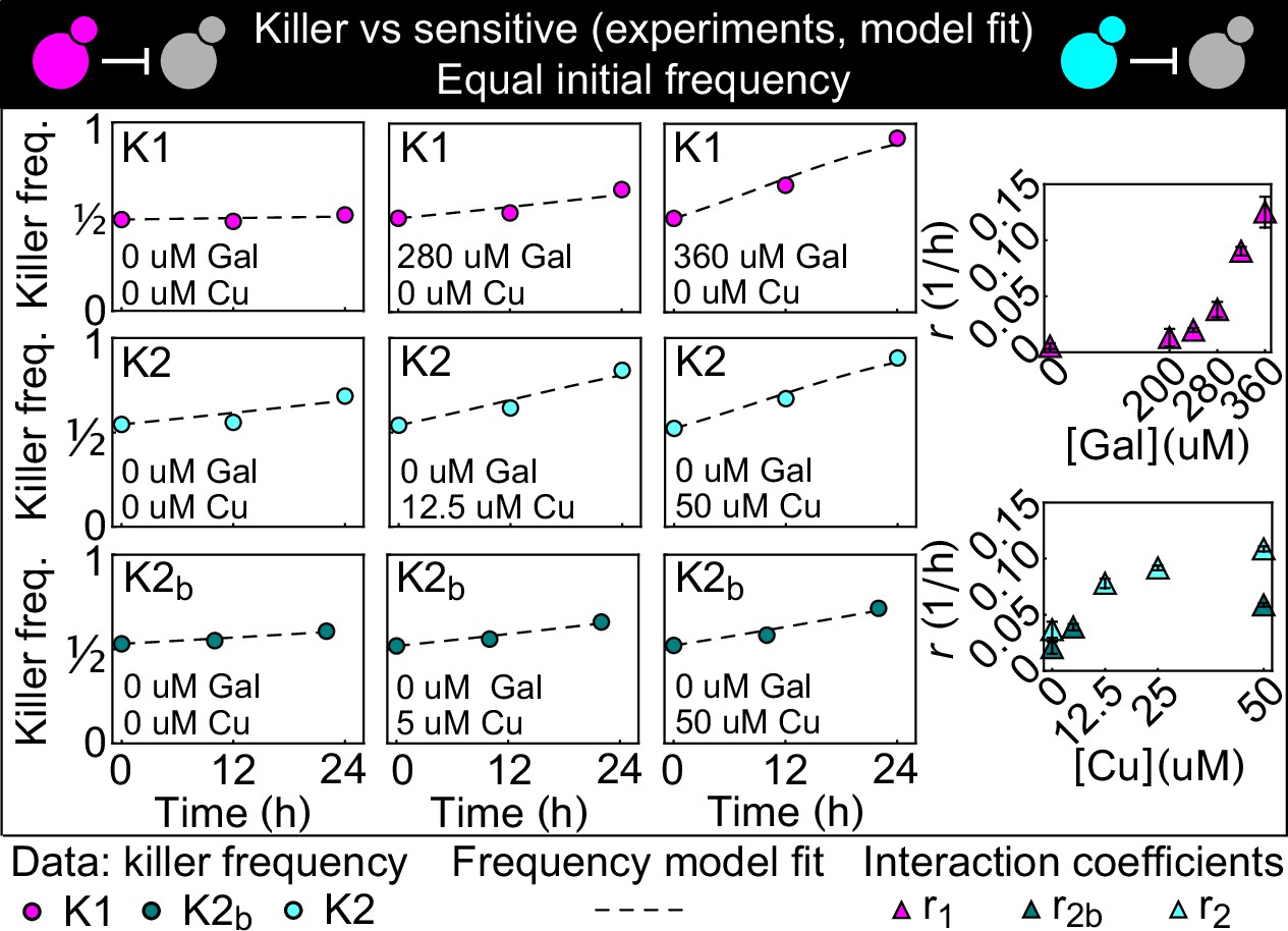
Temporal change of the killer strain frequencies in competition assays against sensitive strains, at different inducer concentrations.
Different colored points depict data corresponding to the killer strains K1 (magenta), K2 (cyan), and K2b (dark green). For each killer strain, increasing its inducer’s concentration increased its killing strength, that is, the rate at which its frequency grew with time. In the absence of inducers, the K1 strain frequency remained constant, whereas strains K2 and K2b still displayed killing activity, which we attribute to the leakiness of the PCUP1 promoter. Each data point is the mean of two, three, or five technical replicates. The x axis reports time since the first measurement. Dashed lines show the best fits of the frequency model Equation 1 and 10. The panels on the right show the best-fit interaction coefficients (which are proportional to toxin production rates) as a function of the inducer concentrations (mean ± SD, Table 3).
-
Figure 2—source data 1
This Excel spreadsheet contains all data used to plot Figure 2 and to compute the interaction coefficients.
The first Excel sheet contains the frequency of the K1 strain in all competition assays against strain S2 at all measurement times and galactose concentrations. The second Excel sheet contains the frequency of the K2 strain in all competition assays against strain S1 at all measurement times and copper concentrations. The third Excel sheet contains the frequency of the K2b strain in all competition assays against strain S1 at all measurement times and copper concentrations. The fourth Excel sheet contains the best-fit estimates for the interaction coefficients (mean ± SD).
- https://cdn.elifesciences.org/articles/62932/elife-62932-fig2-data1-v3.xlsx
Figure 3 with 2 supplements

Comparison between experimental, well-mixed competitions of killer vs killer and model predictions.
(A) Temporal change of strain K1’s frequency in competition assays against strain K2, at different inducer concentrations (only one of the two inducers was added in each replicate). Each data point is the mean of 13 or more technical replicates, error bars are one standard deviation. Solid lines in (A) and (B) are predictions according to Equation 1 with parameters estimated from competitions between the killer strains K1 and K2 and the sensitive, nonkiller strains S1 and S2. Gray bands show the 68% confidence interval for the model. (B) Changes in the frequency of strain K1 following 24 hr of competition against strain K2, at different concentrations of the inducers (subpanels) and at different initial frequencies. The x axis gives the K1 frequency 14 hr after inoculation, the y axis gives the K1 frequency 38 hr after inoculation. The dashed lines show the 1:1 line that points would lie on if the two strains had equal fitness. The critical inoculum corresponds to the intersection point between the dashed lines and the solid lines (model), or an interpolation of the data points (experiment). Insets show the control experiments of competing the two sensitive strains S1 and S2 with each other at the same inducer concentrations as the parent subpanels. The bottom-right subpanel shows the correlation between the value of predicted from our model (the intersection point between the solid and dashed lines) and the experimental value of based on competitions (the intersection of the interpolation between the data points and the dashed lines) for all inducer concentrations. The dotted line is the 1:1 line. (C) Temporal derivative of according to Equation 1, at the inducer concentration values of panel B (left, only the lines corresponding to the highest galactose and highest copper concentrations are labeled) and the corresponding quartic potential (right). (D) At the galactose concentration of 250 µM, the unstable equilibrium is close to 1/2. Different technical replicates that start around tend toward different stable equilibria of Equation 1 (i.e., and ) in the long-term limit, highlighting the instability of the equilibrium point. Yellow points show frequencies of the K1 strain 14 hr after inoculation, green points show frequencies of the K1 strain 38 hr after inoculation.
-
Figure 3—source data 1
This Excel spreadsheet contains all data used to plot Figure 3.
The first Excel sheet contains the frequencies of the K1 strain in competition assays against strain K2 in which the two strains had identical initial frequencies (data shown in panel A). The second Excel sheet contains the frequencies of the K1 strain in competition assays against strain K2 in which the two strains had different initial frequencies (data shown in panel B). The third Excel sheet contains the frequencies of strain K1 in the competition assays with inducer concentration close to 250 µM galactose (data shown in panel D).
- https://cdn.elifesciences.org/articles/62932/elife-62932-fig3-data1-v3.xlsx
Figure 3—figure supplement 1
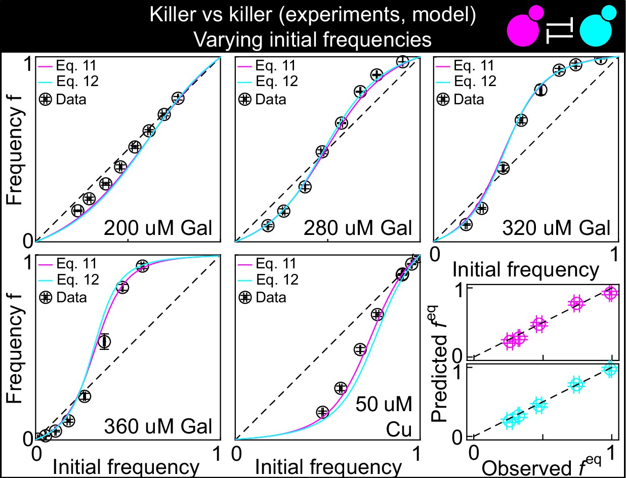
This figure shows the same data as Figure 3B, but with the predictions of the models with Equation 11 (magenta) and Equation 12 (cyan) instead of Equation 1, modified to account for toxin production by both strains, and parametrized using competition assays between the killer strains and sensitive strains (Figure 2): K1 versus S1 and K2 versus S1.
The five larger panels show the changes in the frequency of the K1 strain following a 24 hr growth period, at different concentrations of the inducers and at different initial frequencies. The x axis gives the K1 frequency 14 hr after inoculation, the y axis gives the K1 frequency 38 hr after inoculation. The dashed and dotted lines show the 1:1 line. The critical inoculum corresponds to the intersection point between the solid and the dashed lines. The two smaller, bottom-right panels show the agreement between the predicted values of (the intersection point between the solid line and the 1:1 dashed lines in the larger panels, y axis) and the measured values (the intersection point between an interpolation of the data points and the dashed 1:1 lines, x axis) for all inducer concentrations. Values using Equation 11 are shown in magenta, those for Equation 12 in cyan, with both equations modified to account for toxin production by both strains. Confidence intervals for the model predictions are not shown here because best-fit parameter errors estimated from the stationary Markov Chain distribution are very small and do not affect the model predictions significantly.
Figure 3—figure supplement 2
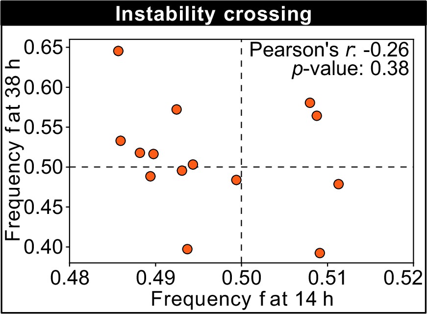
This figure shows the frequency of the K1 killer strain at the first (horizontal axis) and second (vertical axis) measurement time point for different technical replicates of a competition experiment with 250 µM galactose, which is close to the unstable equilibrium and shows replicates that tend toward different stable equilibria in the limit of large times (the same data are plotted in Figure 3D).
No correlation can be detected between the frequencies at the first and second measurement time points, suggesting that the stochasticity of the dynamics is more important than the initial condition when determining which replicates will tend toward different stable equilibria in the limit of large times.
Figure 4
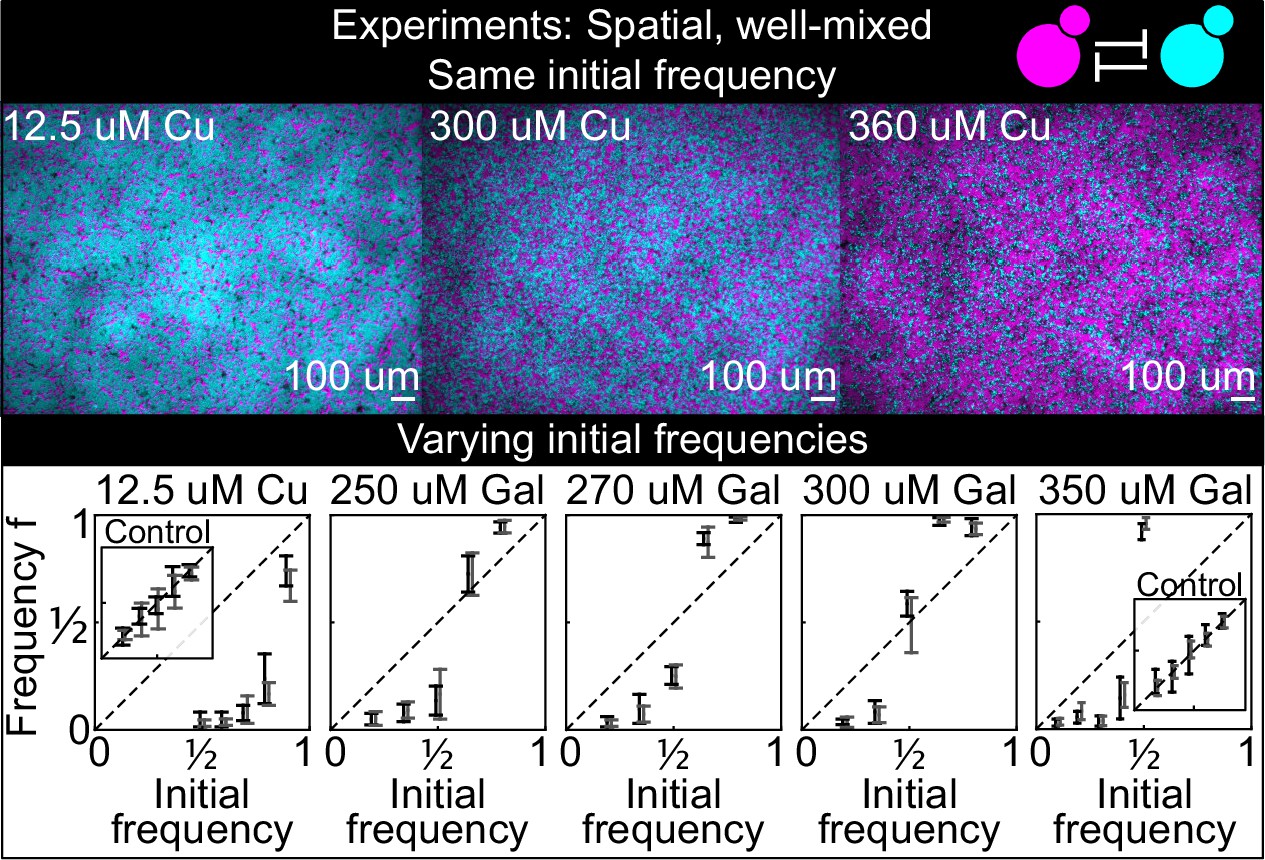
Antagonistic competition of spatially well-mixed, toxin-producing strains K1 and K2 growing on solid agar surfaces, at different inducer concentrations (subpanels) and different initial frequencies.
The upper panels show combined fluorescence images of three representative spatially well-mixed populations imaged 5 hr after inoculation. The images show populations that started at 50:50 initial frequencies of K1 and K2, with K2 outcompeting K1 on the left and the opposite outcome on the right. The lower panels show the relative frequencies of the two strains at the time of inoculation (x axis) and 24 hr after inoculation (y axis), estimated as the relative fraction of space occupied by each strain. Black and gray data show data from two different experiments, and the two whiskers of each data point connect the maximum and the minimum estimated frequency of K1. Due to the difficulty of unequivocally assigning each pixel to one or the other strain in this assay, we report conservative estimates of the maximum and minimum frequencies that we can confidently assign to the K1 strain. The dashed lines show the 1:1 line that points would lie on if the two strains had equal fitness. Insets in the lower subpanels show control experiments: competition assays between the nonkiller strains S1 and S2, at the same inducer concentrations as the parent subpanels.
-
Figure 4—source data 1
This Excel spreadsheet contains all data used to plot Figure 4.
The Excel sheet contains the frequencies of the K1 strain estimated after 24 hr from inoculation, and the corresponding initial frequencies and inducer concentrations. We reported conservative estimates for the minimum and maximum frequency of the K1 strain, due to the difficulty of unequivocally assigning each pixel to one or the other strain in this assay.
- https://cdn.elifesciences.org/articles/62932/elife-62932-fig4-data1-v3.xlsx
Figure 5 with 5 supplements
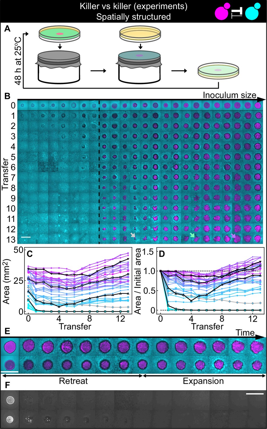
Antagonistic competition of killer strains K1 and K2b in spatially structured populations.
Experiments were performed on agar medium with 360 µM galactose, a concentration at which the K1 strain is a stronger killer than the K2b strain. (A) We used replica plating to replenish nutrients and dilute the populations, while preserving the spatial structure of the population. At the end of each growth period (48 hr at 25°C), the agar plates hosting the experimental populations were gently pressed onto a microfiber cloth laid flat on a cylinder, leaving a diluted copy of the population on the cloth. A fresh agar plate was then pressed onto the same cloth, leading to an effective dilution of the population that preserved its spatial structure. (B) Shown from left to right are spatially structured populations of the invader K1 (magenta) and the resident K2b (cyan) strains originated from depositing droplets of different volumes of K1 onto a lawn of K2b cells. The populations are ordered based on the number of K1 cells at the end of the first growth cycle (estimated from the integrated ymCherry fluorescence of strain K1): the population with the smallest number of K1 cells is on the left, that with the largest number on the far right (first row). Different rows in the same column show the same population 48 hr after the previous transfer. The existence of a critical inoculum size is clearly visible and is marked by a dashed, black line. Populations on the left of this line failed to expand, whereas populations on the right of it persisted and eventually expanded. (B) shows only a subset of the experimental populations; Figure 5—figure supplement 1 shows all the populations. An outlier population (gray arrow) and a population with a re-invading K2b sub-population (green arrow) are discussed in the main text. (C) Area covered by each K1 population at the end of each 48 hr growth period between transfers, color coded from cyan to magenta according to the integrated ymCherry fluorescence intensity of each replica at the end of the first growth period. Highlighted in black are four characteristic curves highlighting the fact that populations above the critical inoculum initially decrease in size, before expanding later. (D) Same data as in (C), divided by the initial area to highlight relative changes. Shown in (E) are two populations in which the retreat and expansion phases of the dynamics are clearly visible. The two rows show two different populations, whereas different columns show the same populations at the end of the growth periods following successive transfers. Both K1 (magenta) and K2b (cyan) populations initially retreat, leaving a region without cells (a black ‘halo’ surrounding the magenta islands). In the expansion phase of the dynamics, the magenta regions expand and increase their area. These populations are well above the critical inoculum size. Panel (F) shows the temporal dynamics of the two largest populations below the critical inoculum (last two columns of panel B before the dashed, black line). The largest population (first row in F) disappeared almost immediately, whereas the second-to-last one (second row) disappeared after five transfers. Only the fluorescence due to strain K1 is shown. Scale bars are 1 cm long. Figure 5—figure supplement 2 shows a control experiment in which we followed the same protocol using the sensitive, nonkiller strains S1 and S2, and found that the areas of S1 inoculations on a lawn of S2 cells remained constant with time, for all initial inoculation sizes.
-
Figure 5—source data 1
This Excel spreadsheet contains all data used to plot Figure 5, Figure 5—figure supplement 1, and Figure 5—figure supplement 2.
The first Excel sheet contains data from spatially structured competitions between strains K1 and K2b (data shown in Figure 5C–D). It reports the integrated ymCherry fluorescence intensity of each replica at the end of the first growth period, and the areas of each K1 population at the end of each growth period, immediately before being transferred to a fresh plate. The second Excel sheet contains data from spatially structured competitions between strains S1 and S2 (data shown in Figure 5—figure supplement 2, panels B–C). It reports the integrated ymCherry fluorescence intensity of each replica at the end of the first growth period, and the areas of each S1 population at the end of each growth period, immediately before being transferred to a fresh plate.
- https://cdn.elifesciences.org/articles/62932/elife-62932-fig5-data1-v3.xlsx
Figure 5—figure supplement 1
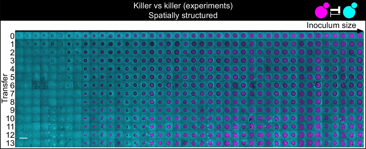
Shown here are all experimental replicates of the experiment of Figure 5.
Shown from left to right are spatially structured populations of the invader K1 (magenta) and the resident K2b (cyan) strains originated from depositing droplets of different volumes on a lawn of K2b cells. The populations are ordered from the one with the smallest number of K1 cells (estimated via the integrated ymCherry fluorescence from strain K1) on the left to the one having the largest initial number of K1 cells at the end of the first growth cycle on the right (first row). Different rows on the same column show the same population 48 hr after the previous transfer. The scale bar is 1 cm long.
Figure 5—figure supplement 2

Non-antagonistic competition of sensitive, nonkiller strains in spatially structured populations.
Experiments were performed in parallel to those of Figure 5, following the same experimental protocol. The strains used here carry the similar genetic constructs to those in the K1 and K2b strains, but without the killer toxin genes, and thus competed solely for nutrients and for space, without direct antagonistic interactions mediated by toxins. The scale bar is 1 cm long. (A) Inoculations of all initial sizes maintained their shape and size throughout the experiment, following successive transfers and 48 hr periods of growth. The populations are ordered based on the number of K1 cells at the end of the first growth cycle (estimated via the integrated ymCherry fluorescence of strain K1): the population with the smallest number of K1 cells is on the left, that with the largest number on the far right (first row). Different rows show the same populations after 48 hr from the previous replica-plating transfer. Panels (B–C) show that the magenta populations maintained their areas, measured at the end of each growth period immediately before a transfer, throughout the entire experiment.
Figure 5—figure supplement 3
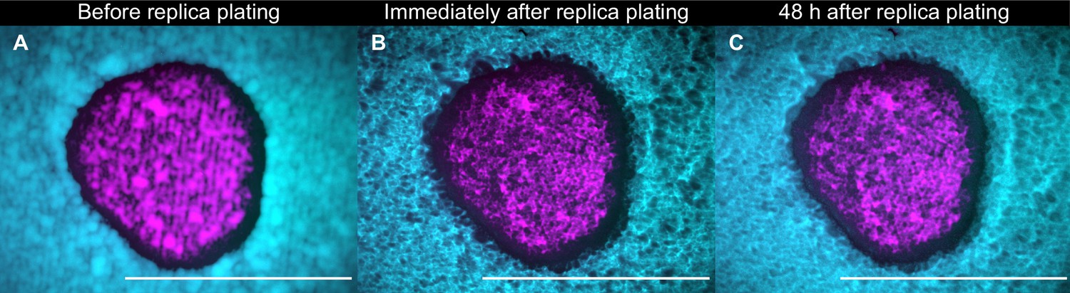
A population of K1 cells (magenta) surrounded by K2b cells (cyan) imaged after 48 hr of growth at 25°C immediately before replica plating (A), immediately after replica plating (B), and after further 48 hr of incubation at 32°C (a temperature at which the K1 and K2 toxins are unstable) following replica plating (C).
Note that panels B and C show the populations that remain on the plate during the replica plating transfer, and not the new, diluted copy of the populations on plates with replenished nutrients. No visible growth in the halo region can be discerned by comparing panels B and C, showing that nutrients are depleted at the end of the 48 hr period of growth between transfers. Scale bars are 1 cm long. These experiments were performed using different batches of medium ingredients compared to the other experiments, and thus the activity of the two toxins and their expression rates (and thus halo widths) may differ from the other experiments.
Figure 5—figure supplement 4
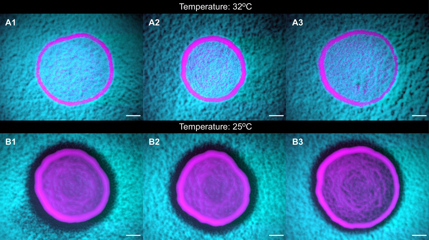
The toxins are unstable at high temperatures.
Panels (A1-3) and (B1-3) show populations of strains K1 and K2b grown at 25°C and at 32°C, respectively, highlighting that the toxin is unstable at 32°C, as shown by the absence of a halo at that temperature, and by the fact that the two strains coexist within the inoculum. Scale bars are 1 mm long. These experiments were performed using different batches of medium ingredients compared to the other experiments, and thus the activity of the two toxins and their expression rates (and thus halo widths) may differ from the other experiments.
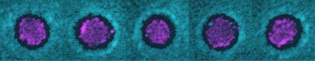
Figure 5—figure supplement 5
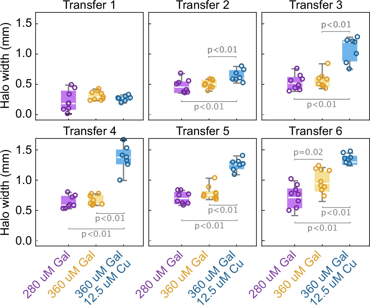
The width of the halo grows with the toxin production rate by the two strains.
Box whisker plots show the width of the halo around different inoculations of the K1 strain on a lawn of K2b cells, at different concentrations of the inducers (no copper was added in the 280 µM Gal and 360 µM Gal treatments), at the end of 48 hr growth periods between transfers. Statistically significant differences in the mean halo widths and the corresponding p-values are highlighted with brackets. These experiments were performed using different batches of medium ingredients compared to the other experiments, and thus the activity of the two toxins and their expression rates (and thus halo widths) may differ from the other experiments.
Figure 6 with 3 supplements
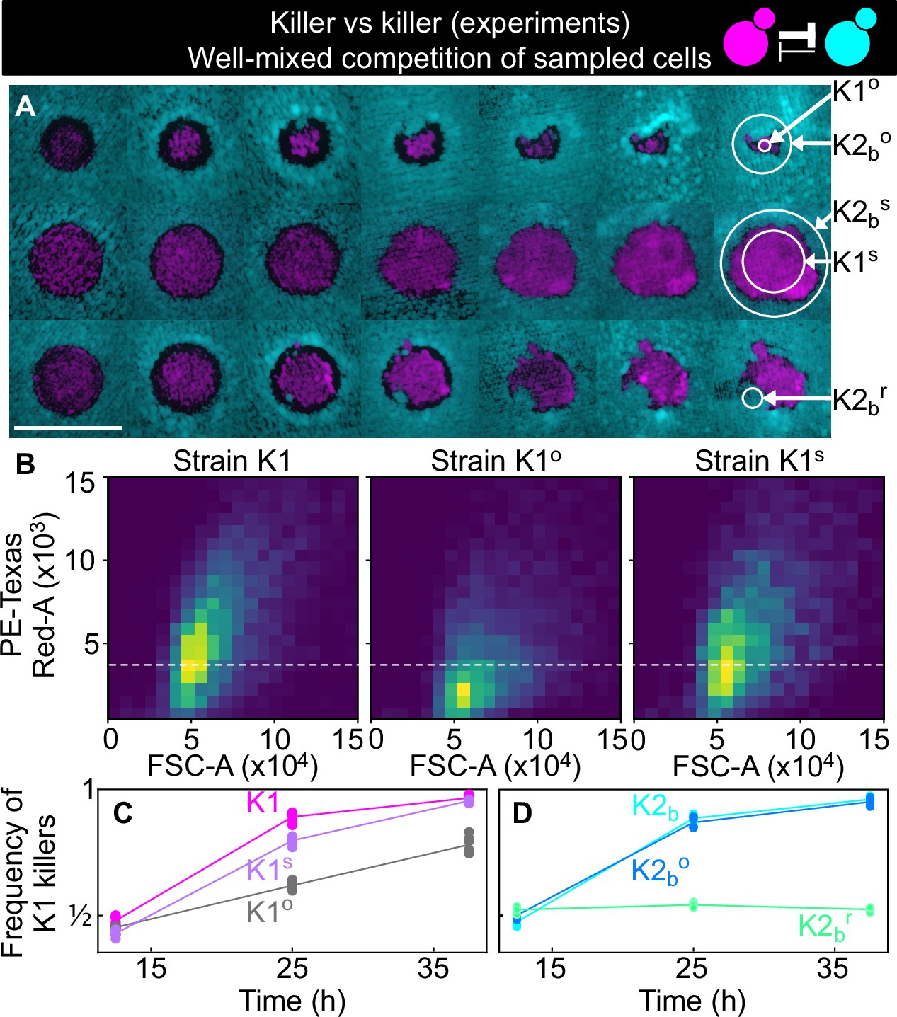
Cells sampled from certain replicates at the end of the experiment shown in Figure 5 showed altered killing strength and toxin resistance.
(A) Regions from which the samples were taken at the end of the experiments of Figure 5. The three rows show the replicates highlighted with gray, purple, and green arrows in Figure 5B, respectively. Different columns show the same populations at every other transfer. The scale bar is 1 cm long. (B) Density histograms of fluorescence intensity (y axis, arbitrary units) versus forward scatter (FSC, x axis, arbitrary units), which correlates with cell size, measured via flow cytometry during competitions in well-mixed liquid cultures between strains K1, K1o, and K1s, versus K2b. K1 is the strain used in all other experiments, K1o and K1s are populations sampled at end of the experiments of Figure 5. The fluorescence intensity of population K1o is lower than that of K1 and K1s. The dashed line shows the K1 histogram mode as a visual aid to compare fluorescent intensities. (C) In competition assays in liquid at 360 µM galactose, the frequency of K1 and K1s competing against strain K2b increases faster than the frequency of K1° competing against K2b, showing that population K1o is a weaker killer than K1 and of other populations that successfully expanded in the experiments of Figure 5 (e.g., K1s). (D) In competition assays in liquid at 360 µm galactose, strain K1 competing against strain K2b (cyan) and strain K1 against the sub-population K2bo (light blue) sampled at the end of the experiment of Figure 5 follow similar dynamics suggesting that the collapse of K1o was not due to increased toxin production by K2bo, or it developing resistance to the K1 toxin. The competition assay with strain K1 against strain K2br (green), which re-invaded a K1 population in the experiments of Figure 5, instead, showed no increase in frequency for strain K1, suggesting that K2br developed resistance to the K1 toxin. Different data points in (C–D) show different technical replicates.
-
Figure 6—source data 1
This Excel spreadsheet contains all data used to plot Figure 6 and Figure 6—figure supplement 1.
Each Excel sheet contains the frequencies of the K1 killer strain (K1, K1s, or K1o depending on the treatment) in each of the competition assays shown in Figure 6C–D, which were performed with the same initial frequency for the two strains. The last two Excel sheets contain data from the competition assays shown in Figure 6—figure supplement 1A-B, which were performed with different initial frequencies for the two competing strains.
- https://cdn.elifesciences.org/articles/62932/elife-62932-fig6-data1-v3.xlsx
Figure 6—figure supplement 1
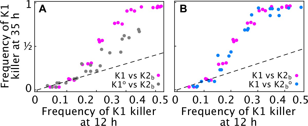
The population K1o isolated from the outlier replicate of Figure 5B-D is a weaker antagonist than the ancestor strain K1.
(A) Competition assays performed in liquid with 360 µM galactose at different initial frequencies of the K1 killer strains versus strain K2b show that cells sampled from the outlier population K1o (gray) increase in frequency more slowly than the ancestor K1 strain (magenta) for all initial frequencies, suggesting that K1o is a weaker killer than the ancestor strain K1. The x axis gives the K1 frequency 12 hr after inoculation, the y axis gives the K1 frequency 35 hr after inoculation. (B) Competition assays performed in liquid with 360 µM galactose at different initial frequencies of the killer strain K1 versus strain K2b (magenta) and K2bo (K2 cells sampled from the region around the outlier population K1o, light blue) show that K2b and K2bo cells have comparable killer strengths, given that their frequency falls (seen as a rise in the frequency of strain K1) at similar rates. Different dots show measurements from different technical replicates. Dashed lines are 1:1 lines.
Figure 6—figure supplement 2
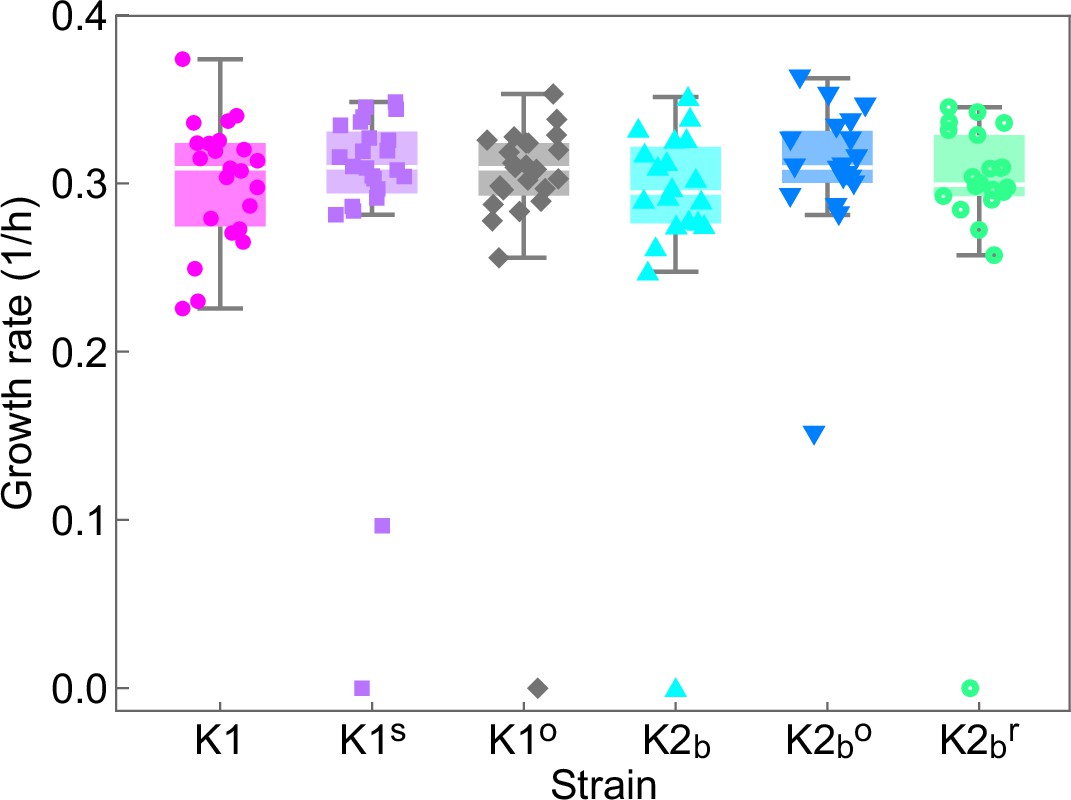
Single-cell growth rates of the ancestor strains (K1, K2b) and of cells isolated at the end of the experiment of Figures 5 and 6 (K1s, K1o, K2bo, K2br) grown on YPD agar plates identical to the ones used for the experiments of Figures 5 and 6, but in the absence of inducers.
Droplets of each strain were deposited on a plate on a grid at distances of 1 cm from each other and the location of each strain within the grid was randomized. Cells on the plate were imaged using an inverted microscope with 50× objective every 20 min for 6 hr, during which the plate was kept at 25°C using a stage-top incubator. During the 6 hr, cells formed micro-colonies of up to 32 cells, except for a few non-dividing or very slow dividing cells that we excluded from the analysis, but whose growth rates are shown in the plot. Data points show growth rates obtained by fitting exponential growth curves to experimental data for the number of cells in individual micro-colonies. t-Tests performed between all pairs of strains/mutants gave no statistically significant differences between their growth rates (all corresponding p-values are larger than 0.05). Box whiskers plots show the median growth rate (white horizontal lines), the 25% and 75% percentiles (colored boxes), and the maximum and minimum growth rate for each strain (whiskers). Slow- and non-growing cells treated here as outliers have not been included in the computation of medians, percentiles, and minima/maxima.
Figure 6—figure supplement 3
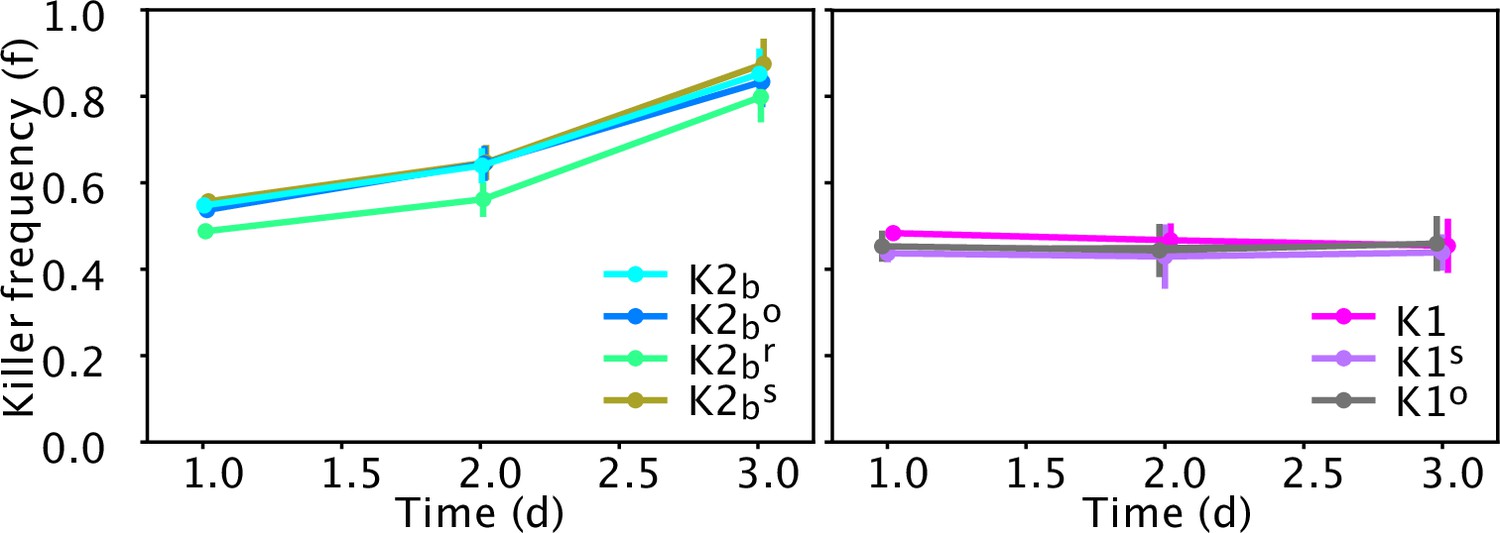
Relative frequency of the ancestor strains (K1, K2b) and of cells isolated at the end of the experiment of Figures 5 and 6 (K1s, K1o, K2bo, K2br) in competition against sensitive strains in well-mixed liquid cultures diluted daily in YPD medium, in the absence of inducers.
Data points show the relative frequency of killer strains across 12 technical replicates, error bars are standard deviations. The left panel shows competitions between cells with the K2 killer toxin gene against the sensitive strain S1, the right panel shows competitions between strains with the K1 killer toxin gene against the sensitive strain S2. Experiments were initialized with a 50:50 mixture of two overnight cultures of each strain and were measured after 1, 2, and 3 days from inoculation, right before dilution. Mixed competition assays performed with strains carrying the K1 killer toxin gene induced by the promoter PGAL1 (strains K1, K1s, and K1o) versus strain S2 can be used to directly detect differences in reproductive fitness, because no toxin is produced in the absence of inducer (galactose) and thus the relative frequency of the two strains varies due to differences in reproductive fitness alone. Mixed competition assays between strains carrying the K2 killer toxin gene induced by the promoter PCUP1 (K2b, K2br, and K2bo) versus strain S1, instead, can only detect the joint effect of differences in reproductive fitness and killer activity, given that the promoter PCUP1 has non-zero expression even in the absence of inducer (copper). t-Tests performed between all pairs of competitions between killer strains/mutants of the same type (i.e., expressing either the K1 or K2 toxin) and the corresponding sensitive strains (figure below) give no statistically significant differences between the rates at which the relative frequency of killer strains in competition assays vary with time (all corresponding p-values are larger than 0.05). These experiments were performed using different batches of medium ingredients compared to the other experiments, and thus the activity of the two toxins and their expression rates may differ from the other experiments.
Figure 7 with 4 supplements
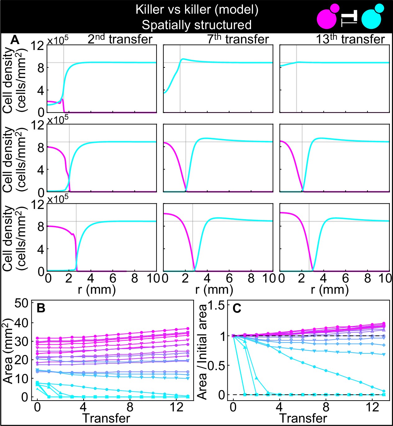
Numerical integrations of the spatial model (Equations 7–9), parametrized using the experiments of Figure 2, and other values taken from the literature, can qualitatively reproduce the experimental dynamics of antagonistic competition between strains K1 and K2b in spatially structured populations.
(A) Simulated K1 inoculations smaller than the critical inoculum (first row) expanding on a landscape occupied by strain K2b fail to establish and expand, whereas larger inoculations do (second and third row). The model can reproduce the formation of the halo, a region without cells at the interface between the two strains (second and third row). (B) Area covered by each simulated K1 population expanding on a landscape occupied by strain K2b at the end of each 48 hr growth period between simulated transfers, color-coded from cyan to magenta according to the total K1 population of each replica at the end of the first growth period. (C) Same data as in (B), divided by the initial area to highlight relative changes. Compare (B) and (C) to Figure 5C and D.
Figure 7—figure supplement 1
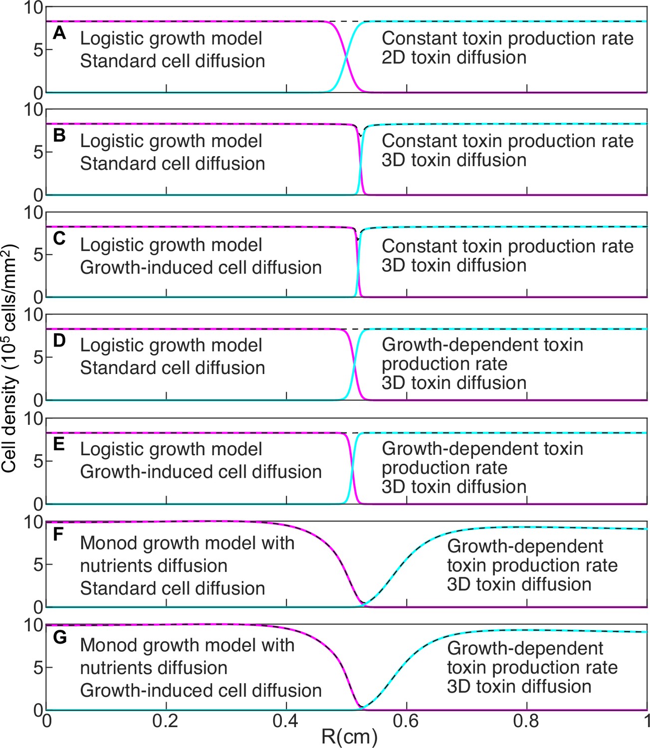
Models that do not account for nutrient diffusion fail to reproduce the formation of the halo between two antagonist strains.
Magenta and cyan curves show the density profiles of K1 and K2 killer strains. The dashed, black lines show the total cell density and are the sum of the magenta and cyan density profiles. All models were parametrized using competition experiments between killer and sensitive strains, and parameters corresponding to strains K1 and K2b competing with 360 µM galactose and 0 µM copper were used. In the initial conditions strain K1 occupied the entire region and strain K2b occupied the region , with mm. The figures show density profiles after six transfers. The model in panel A corresponds to Equation 6. The model in panel G corresponds to Equations 7–9. The characteristic features of intermediate models are reported in each panel.
Figure 7—figure supplement 2
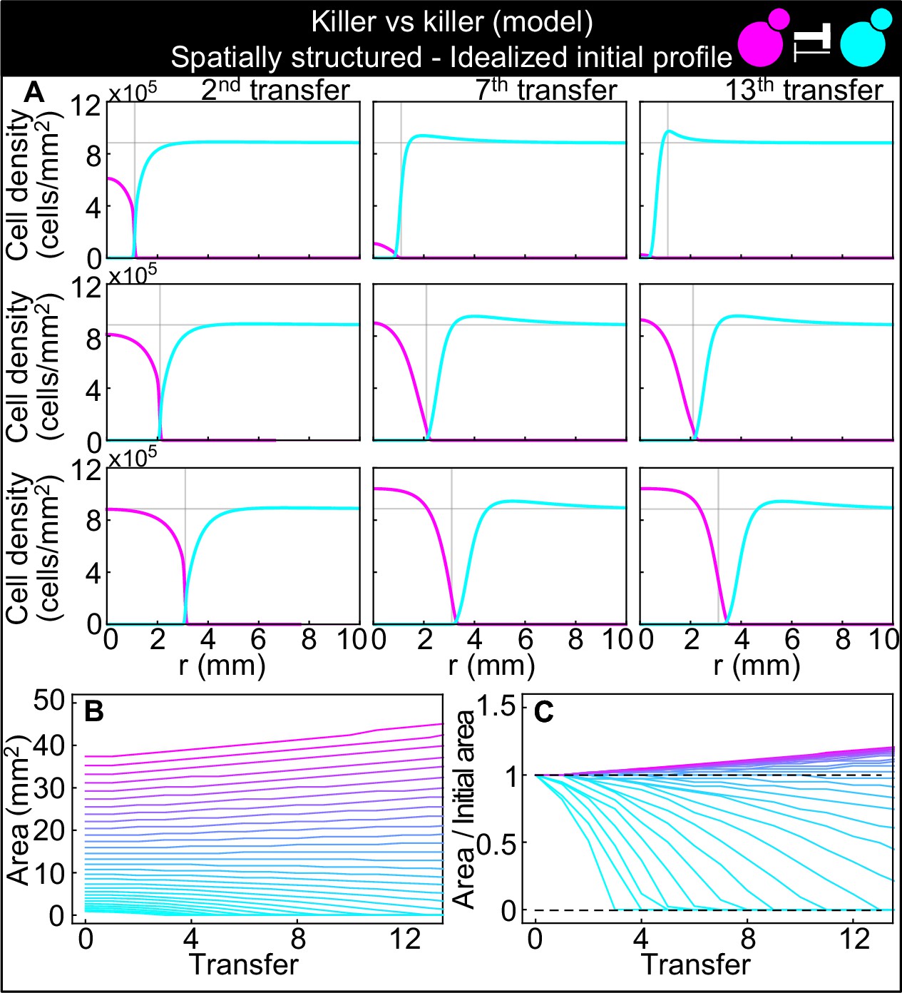
Numerical integrations of the spatial model (Equations 7–9), parametrized using the experiments of Figure 2 and other values taken from the literature, can qualitatively reproduce the experimental dynamics of antagonistic competition between strains K1 and K2b in spatially structured populations.
Same plots as Figure 7, but with idealized initial conditions in which strain K1 occupied the entire region and strain K2b occupied the region , where the initial radius was varied between 5 and 34 mm. (A) Simulated K1 inoculations smaller than the critical inoculum (first row) expanding on a landscape occupied by strain K2b fail to establish and expand, whereas larger inoculations do (second and third row). The model reproduces the formation of the halo, a region without cells at the interface between the two strains (second and third row). (B) Area covered by each simulated K1 population expanding on a landscape occupied by strain K2b at the end of each 48 hr growth period between simulated transfers, color-coded from cyan to magenta according to the total K1 population of each replica at the end of the first growth period. (C) Same data as in (D), divided by the initial area to highlight relative changes. Comparison with Figure 7B and C shows that the presence of K2 cells within the K1 inoculum leads to faster extinction of K1 cells in inocula below the critical size, is required for the initial retreat of K1 populations above the critical size, and leads to a more abrupt transition between the dynamics of K1 populations that go extinct and those that thrive.
Figure 7—figure supplement 3
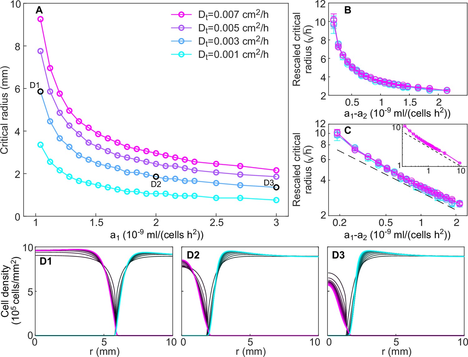
Dependence of critical radius size on model parameters.
(A) Size of the critical radius for different values of the toxin production rate of the invader strain and of the toxin diffusion rate (different curves), for a fixed value of the toxin production rate of the resident strain, mL/(cell hr2) in numerical simulations of the model (Equations 8; 9), starting from idealized initial conditions as for Figure 7—figure supplement 2. Critical radii were computed by integrating Equation 8–9 over 20 consecutive transfers for different values of the inoculum radius (varied with step size 0.1 mm), measuring the total number of K1 cells at the end of each transfer, and identifying the largest and lowest values of the inoculum radius such that the total number of K1 cells was decreasing and increasing, respectively, in the last five transfers. Panels (B–C) show that curves corresponding to different values of the toxin diffusion coefficient collapse onto a single curve when dividing the critical radius by a factor . In panel B, rescaled critical radii and are plotted in linear scale. In panel C, rescaled critical radii are plotted in log-log scale versus the difference between the invader and resident strain toxin production rates , to highlight the approximate power-law dependence for large values of (the dashed black line is proportional to ). The inset of panel C shows that the power-law behavior extends to mL/(cell hr2) (only data for cm2/hr and cm2/hr are shown because smaller values of would require a smaller radial integration step). (D1–D3) Density profiles of the two strains at the end of each growth period between transfers (black curves), starting from uniform spatial distributions of the invader strain within the critical radius and of the resident strain outside the critical radius. Shown in magenta and cyan are the stationary density profiles of the two strains in the limit of large times, after the profiles have reached stationarity.
Figure 7—figure supplement 4
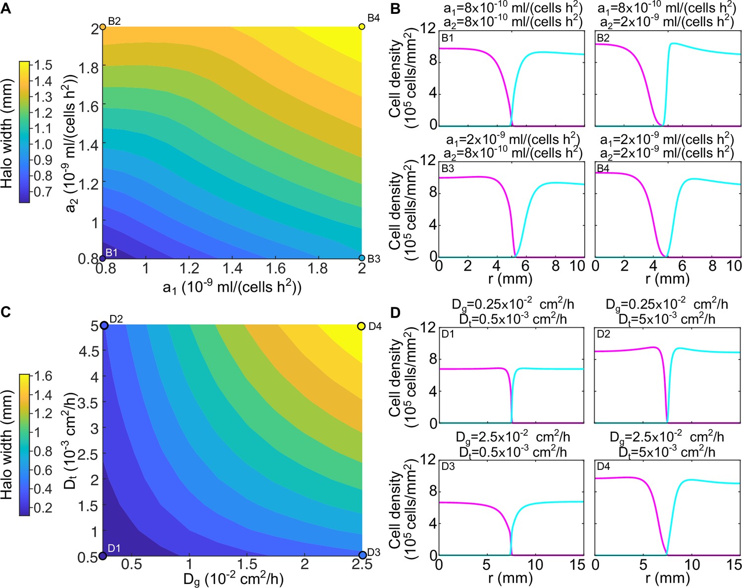
The width of the halo and the shape of the two strains’ density profiles varies with the parameters of the model.
(A) Width of the halo region between the invader and the resident strain for different values of the toxin production rates and in numerical simulations of the model (Equations 8; 9). The halo width was measured as the distance between the radius at which the resident density profile reaches half its maximum and the radius at which the invader density profile reaches half its maximum. (B) Density profiles of the two strains for different values of the toxin production rates, corresponding to the points highlighted in panel A. (C) Width of the halo region between the invader and the resident strain for different values of the toxin diffusion rate and the glucose diffusion rate in numerical simulations of the model (Equation 8–9), with the toxin production rates set to mL/(cell hr2). (D) Density profiles of the two strains for different values of the toxin and glucose diffusion rates, corresponding to the points highlighted in panel C. In all the panels, the populations were diluted every 48 hr and the halo width was measured after five dilutions. In the initial conditions strain K1 occupied the entire region and strain K2b occupied the region , with cm.
Author response image 1
An increased fluorescent intensity was often observed at the two sides of the halo, corresponding to a thicker layer of cells in those regions compared to anywhere else on the plate.
Modeling suggests that such thicker layer of cells is due to nutrient diffusion away from the halo.
Tables
Key resources table
| Reagent type (species) or resource | Designation | Source or reference | Identifiers | Additional information |
|---|---|---|---|---|
| Strain, strain background (Saccharomyces cerevisiae) | W303 | Murray lab | W1588 | The complete list of derived strains is available in Table 2 |
| Chemical compound, drug | Copper(II) sulfate pentahydrate | Sigma Aldrich | C8027 | |
| Chemical compound, drug | D-(+)-Galactose | VWR | VWRV0637 | |
| Chemical compound, drug | Ethylene glycol-bis(β-aminoethyl ether)-N,N,N′,N′-tetraacetic acid (EGTA) | Sigma Aldrich | E34378 | |
| Software, algorithm | Fiji (ImageJ) | PMID:22743772 | ||
| Software, algorithm | FlowCytometryTools | https://eyurtsev.github.io/FlowCytometryTools/, (Friedman and Yurtsev, 2013) | Version 0.5.0 | |
| Software, algorithm | Mathematica | Wolfram | SCR_014448 | Version 12.1.0.0. Custom scripts available at https://github.com/andreagiometto/Giometto_Nelson_Murray_2020 |
| Software, algorithm | Matlab | Mathworks | RRID:SCR_001622 | Version R2018a. Custom scripts available at https://github.com/andreagiometto/Giometto_Nelson_Murray_2020 |
| Software, algorithm | Python | Python | RRID:SCR_008394 | Custom scripts available at https://github.com/andreagiometto/Giometto_Nelson_Murray_2020 |
Table 1
Oligos used in this study.
Oligo name | Oligo sequence |
|---|---|
| oAG5 | ATTACAGCGTGCCACAGATG |
| oAG13 | AATTCTCCACACATAATAAGTACGCTAATTAAATAAAATGCGTACGCTGCAGGTCGAC |
| oAG14 | ACCTTCTTGTTGTTCAAACTTAATTTACAAATTAAGTTTAATCGATGAATTCGAGCTCG |
| oAG15 | TTCGCCACTGTCTTATCTAC |
| oAG17 | CCCGTGAATTTCTAACAAAG |
| oAG22 | ATCCAGTTTAAACGAGCTCGGTAAAGAGCCCCATTATCTTAGC |
| oAG23 | ACTTGGGTTGGCTTCGTCATGTTTTTTCTCCTTGACGTTAAAG |
| oAG24 | TAACGTCAAGGAGAAAAAACATGACGAAGCCAACCCAAGT |
| oAG25 | AGGCCACTAGTGGATCTGATAGCTTGCAAATTAAAGCCTTC |
| oAG26 | AAAACAAACTGTAACGAATTATGAAAGAGACTACCACCAG |
| oAG27 | ATCCAGTTTAAACGAGCTCGCATTACCGACATTTGGGCGC |
| oAG28 | CTGGTGGTAGTCTCTTTCATAATTCGTTACAGTTTGTTTTTCTTAATATC |
| oAG29 | GAAGCTCGCCCTTAGATCTGATTTATATCCTATCCTAGCCGC |
| oAG31 | GGCTAGGATAGGATATAAATCAGATCTAAGGGCGAGCTTC |
| oAG39 | CCAGATGCGAAGTTAAGTGC |
| oAG44 | CTTTGGTGGGTTGAAGAAGG |
| oAG45 | GATCAATCTCTTGCAGCCAC |
| oAG46 | AAGCGATGATGAGAGCGACG |
Table 2
Strains used in this study.
All strains are in the Saccharomyces cerevisiae W303 background. Strain yAG75 has not been used in the experiments but is reported here because it is the ancestor of all the other strains; only those elements that differ from yAG75 are listed for the other yAG strains.
| Strain | Genotype | Note |
|---|---|---|
| yAG75 | MATa BUD4-S288C can1-100 gal1/10Δ::LEU2 his3-11,15 PGAL3Δ::HIS3-MX6-PACT1-GAL3 ura3Δ0 hxk2Δ::HphMX4 | Sensitive to killer toxins K1 and K2, ancestor of all other strains |
| yAG82 | yAG75, PACT1-ymCitrine-TADH1 PTEF-KanMX6-TTEF PCUP1-K2-TCYC1 | Strain K2b, yAG75+ pAG14 |
| yAG83 | yAG75, PACT1-ymCitrine-TADH1 PTEF-KanMX6-TTEF PCUP1-K2-TCYC1 | Strain K2, yAG75+ pAG14 |
| yAG94 | yAG75, PACT1-ymCherry-TADH1 PTEF-KanMX6-TTEF PGAL1-K1-TCYC1 | Strain K1, yAG75+ pAG11 |
| yAG96 | yAG75, PACT1-ymCherry-TADH1 PTEF-KanMX6-TTEF | Strain S1, yAG75+ pAG3 |
| yAG99 | yAG75, PACT1-ymCitrine-TADH1 PTEF-KanMX6-TTEF | Strain S2, yAG75+ pAG5 |
| F166 | MATα leu1 kar1 L-A-HNB M1 [K1+] | Reference K1 strain |
| EX73 | MATa/α HO/HO L-A M2 [K2+] | Reference K2 strain |
Table 3
Best-fit estimates for the parameters of the frequency model Equation 10 fitted to the data from competition assays between toxin-producing strains and sensitive, nonkiller ones.
Concentrations of the inducers galactose (Gal) and copper (Cu) are indicated as superscripts, whereas the parameters , , and (i.e., the parameter in Equation 10 for the strains K1, K2, and K2b) are given in units of 1 /hr (mean ± SD).
| 0.005±0.002 | 0.013±0.008 | 0.020±0.002 | 0.038±007 | 0.090±0.004 | 0.125±0.014 | |
| 0.037±0.007 | 0.078±0.004 | 0.092±0.002 | 0.109±0.002 | 0.021±0.005 | 0.039±0.003 | 0.059±0.002 |
Table 4
Best-fit estimates for the parameters of the full model with logistic growth Equation 11 fitted to the data from competition assays between toxin-producing strains and sensitive, nonkiller ones, via Markov Chain-Monte-Carlo (MCMC).
Concentrations of the inducers galactose (Gal) and copper (Cu) are indicated as superscripts. The parameters and correspond to the rescaled parameter of Equation 11 for the strains K1 and K2, respectively.
| hr–1 | mL/cell/hr2 | ||
| cells/mL | mL/cell/hr2 | ||
| mL/cell/hr | mL/cell/hr2 | ||
| mL/cell/hr2 | mL/cell/hr2 | ||
| mL/cell/hr2 | mL/cell/hr2 | ||
| mL/cell/hr2 | mL/cell/hr2 | ||
| mL/cell/hr2 | mL/cell/hr2 | ||
| mL/cell/hr2 | mL/cell/hr2 |
Table 5
Best-fit estimates for the parameters of the model with Monod growth dynamics Equation 12 fit to the data from competition assays between toxin-producing strains and sensitive, nonkiller ones, via Markov Chain-Monte-Carlo (MCMC).
Concentrations of the inducers galactose (Gal) and copper (Cu) are indicated as superscripts. The parameters , , and correspond to the rescaled parameter in Equation 12 for the strains K1, K2, and K2b, respectively.
| 1/hr | mL/cell/hr2 | ||
| cells/(g glucose) | mL/cell/h2 | ||
| mL/cell/hr1 | mL/cell/h2 | ||
| Set to 0 mL/cell/hr2 | mL/cell/h2 | ||
| mL/cell/hr2 | mL/cell/h2 | ||
| mL/cell/hr2 | mL/cell/h2 | ||
| mL/cell/hr2 | mL/cell/h2 | ||
| mL/cell/hr2 | mL/cell/h2 |
Table 6
Values used in the numerical integrations of Equations 6–9 for the diffusion coefficients and Monod’s constant for growth of Saccharomyces cerevisiae on glucose.
The value of was taken from Postma et al., 1989. As an estimate for the K1 and K2 toxins diffusion coefficient, we took a typical value for proteins of size similar to the K1 and K2 toxins (Magliani et al., 1997) diffusing in agar gels at 25°C (Pluen et al., 1999). The yeast diffusion coefficient was estimated as discussed in the text. The value for was taken from Longsworth, 1955.
| cm2/hr | cm2/hr | cm2/hr | g glucose/mL |
Additional files
Download links
A two-part list of links to download the article, or parts of the article, in various formats.
Downloads (link to download the article as PDF)
Open citations (links to open the citations from this article in various online reference manager services)
Cite this article (links to download the citations from this article in formats compatible with various reference manager tools)
Antagonism between killer yeast strains as an experimental model for biological nucleation dynamics
eLife 10:e62932.
https://doi.org/10.7554/eLife.62932


