How oscillating aerodynamic forces explain the timbre of the hummingbird’s hum and other animals in flapping flight
- Mechanical Engineering, Stanford University, United States
- Electrical Engineering, Eindhoven University of Technology, Netherlands
- Engineering, Sorama, Netherlands
Figures
Figure 1
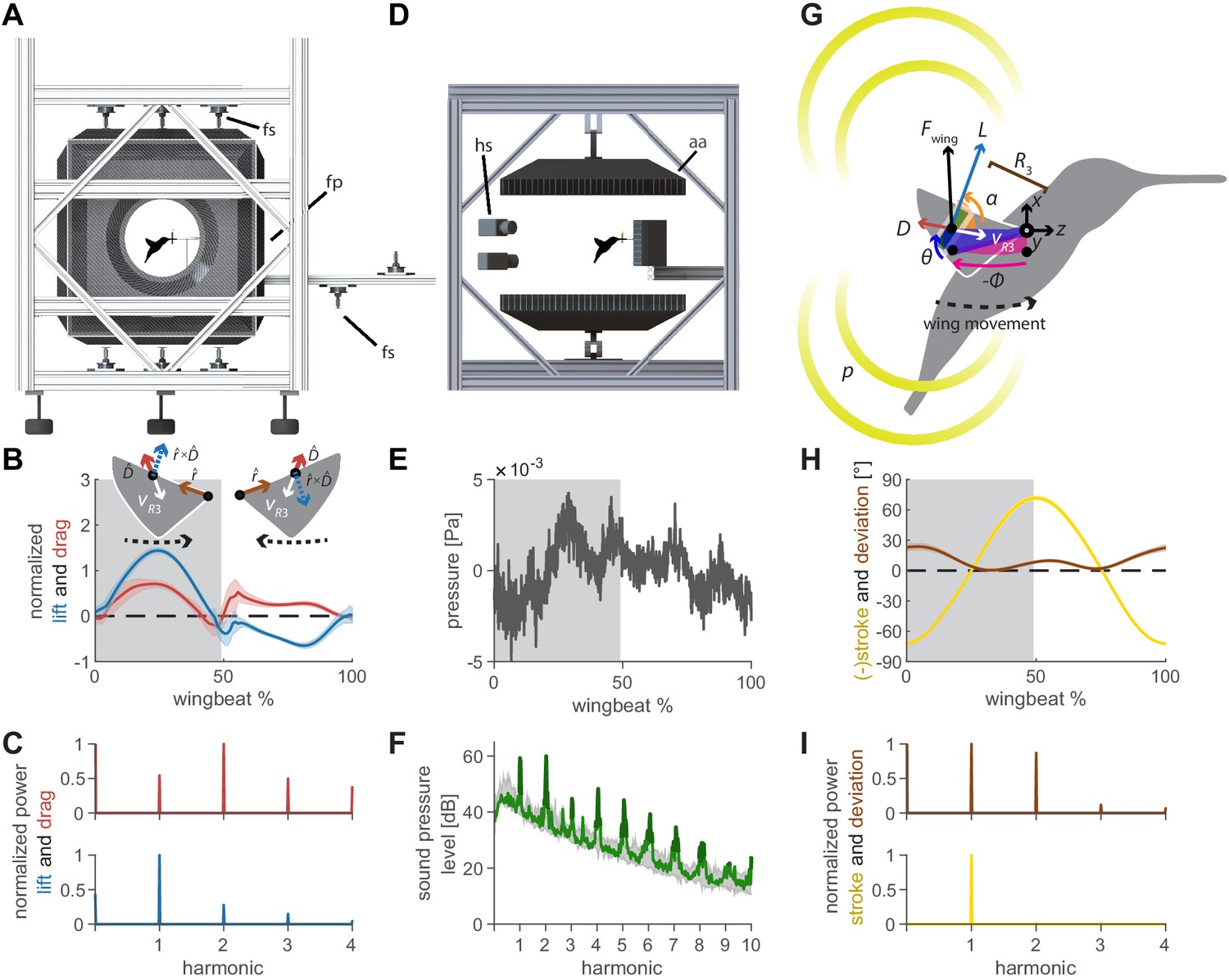
Oscillating aerodynamic force and acoustic field measurements to determine how hummingbirds hum.
(A) 3D aerodynamic force platform setup to measure the forces generated by a hovering hummingbird. Each of the flight arena's walls comprises a force plate (fp) instrumented by three force sensors (fs), two additional force sensors instrument the perch. The six DLT calibrated cameras imaging through three orthogonal ports in pairs are not shown. (B) The lift and drag force generated by hovering hummingbirds during a wingbeat (gray area, downstroke; mean ± std based on N = 6 birds, each bird made two flights, n = 5 wingbeats were fully analyzed per flight for 60 total wingbeats). Lift is negative during the upstroke since the direction of the lift vector is perpendicular to the wing velocity while the drag vector is parallel and opposite to the wing velocity direction, resulting in the lift vector being defined as the cross product of the wing velocity direction and the drag direction (inset). (C) Most of the frequency content in the lift profile is contained in the first harmonic and corresponds to the high forces generated during downstroke (first harmonic mean ± standard deviation is 44.2 ± 1.8 Hz across all birds and flights). In contrast, the frequency content in the drag profile is contained primarily in the second harmonic and corresponds to the equivalent drag generated during the up and downstroke. (D) Acoustic flight arena in which hovering hummingbirds (N = 6 birds, n = 2 flights per bird) were surrounded by four acoustic arrays (labeled aa; 2 ×1024 and 2 × 64 microphones) and four high-speed cameras (hs) while feeding from a stationary horizontal flower (separate experiment with six other individuals). (E) Throughout a wingbeat, each microphone records the local acoustic field generated by the hovering hummingbird (microphone located at the center above bird #1). (F) To generate a representative spectrum of a single bird, the signals of all microphones in all arrays around the bird were summed (green line: N = 1, n = 1) and plotted up to the tenth harmonic. The background spectrum of the lab (range over all trials) is plotted in gray, showing the hum consists primarily of tonal noise higher than the background at wingbeat harmonics (dark green line, 3 dB above maximum background noise). In addition, several smaller non-harmonic tonal peaks can be observed between the first and fourth harmonic with a dB level equivalent to the sixth - seventh harmonic. (G) To determine the acoustic source of the hum, we constructed a simple model that predicts the acoustic field. The acoustic waves radiate outwards from the overall oscillating force () generated by each wing, which can be decomposed into the lift () and drag () forces generated by each wing (recorded in vivo, B). To predict the aeroacoustics, these forces are positioned at the third moment of inertia of the wing () and oscillate back and forth due to the periodic flapping wing stroke (φ) and deviation angle (θ) (recorded in vivo, H). Angle of attack is defined for modeling flapping wing hum across flying species (Figure 4). (I) Hummingbird wing kinematics (φ, θ) measured in vivo from the 3D aerodynamic force platform experiment (gray area, downstroke; mean ± std based on N = 6 birds, n = 2 flights). (I) Whereas most of the frequency content in the stroke profile is contained in the first harmonic, the content in the deviation profile extends to the second and third harmonics.
Figure 2 with 7 supplements
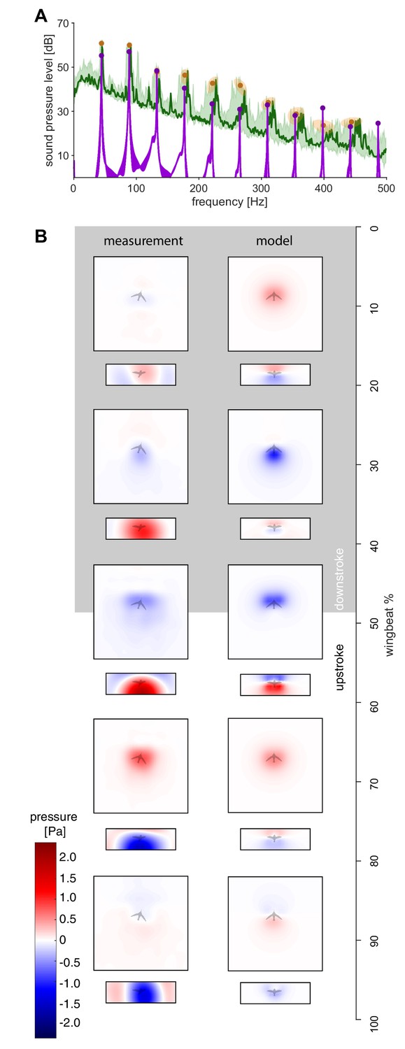
The measured spectra and holograms match those predicted by the simple aeroacoustics model.
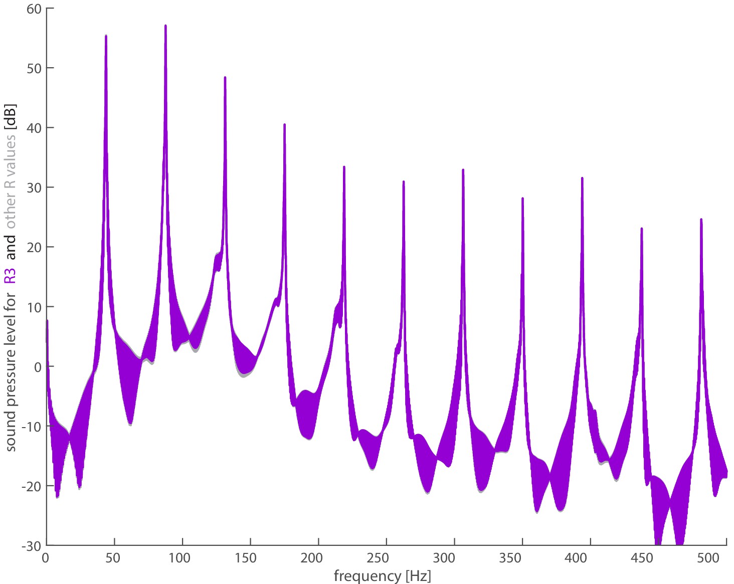
(A) A representative acoustic spectrum measured from all arrays for hummingbird #1 in hover is shown in dark green (n = 1), while the range for N = 6 hummingbirds is shown in light green. The variation in the frequency and sound pressure level (SPL) peak value associated with each harmonic is shown with orange circles (mean) and ellipsoids (width and height, 68% confidence intervals; their asymmetric shape stems from computing the covariance in Pascals while the spectrum is in dB). The peak sound pressure levels predicted by our acoustic model (purple line) match those of the measured spectrum up to higher harmonics. In addition, several smaller non-harmonic tonal peaks can be observed between the first and fourth harmonic with a dB level equivalent to the sixth - seventh harmonic. The predicted spectrum starts at the numerical noise floor, of which the amplitude (< −10 dB) is physically irrelevant. (B) Acoustic holograms throughout the example wingbeat for hummingbird #1 (Figure 1E,F) are presented side-by-side as measured (left) and modeled (right) for the top and front array microphone positions. There is reasonable spatial and temporal agreement between the measured and predicted acoustic nearfield centered around stroke transition (30–70%) where the pressure transitions from minimal (blue) to maximal (red).
Figure 2—figure supplement 1
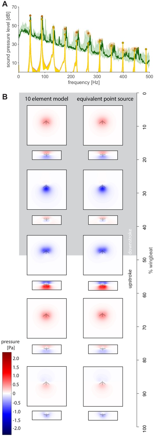
Spectra and holograms show agreement between a 10-element distributed source model and the equivalent single point source model.
(A) The distributed source model uses 10 equally spaced wing elements along the length of the wing (gold; spanwise force distribution adapted from a high-fidelity model from Ingersoll and Lentink, 2018), while the equivalent point source model uses a single point force at (purple). The median difference between the point force and distributed model is 0.1 dB (Supplementary file 2). (B) Acoustic holograms throughout the wingbeat are presented side-by-side for the distributed point model and single point source model (comparison based on top and front microphone array positions).
Figure 2—figure supplement 2
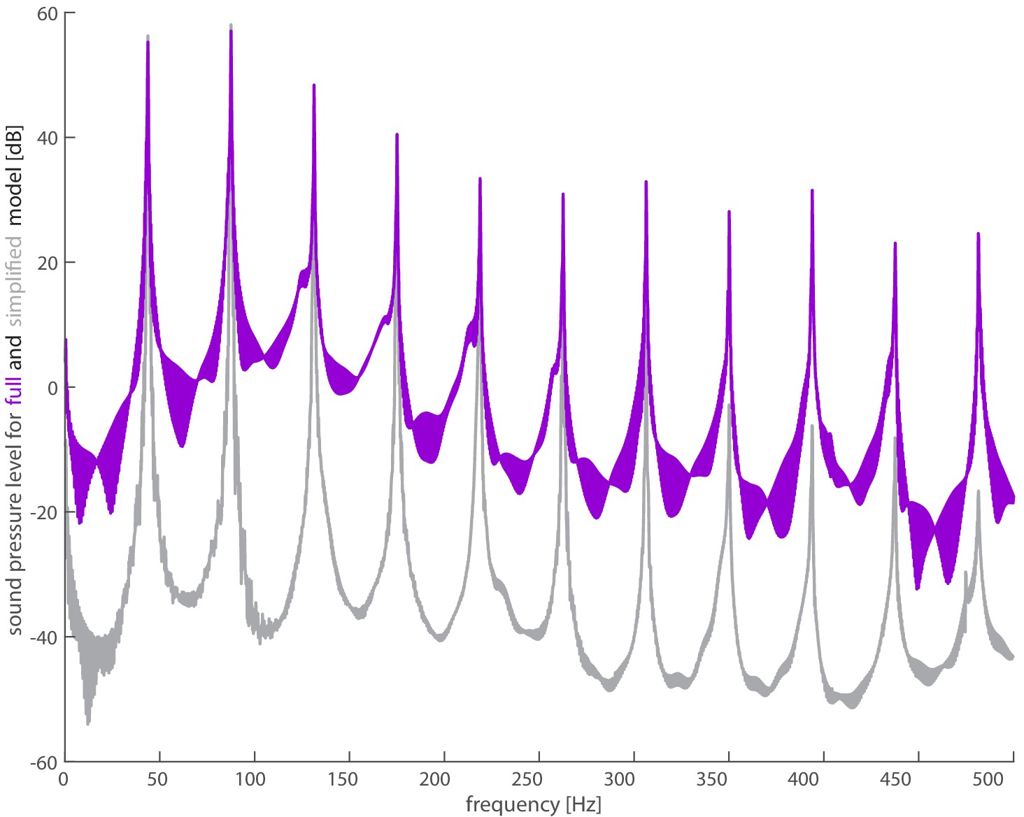
Spectra shows good agreement between full model and simplified model.
The full acoustic model (purple) uses 3D kinematics and lift and drag forces calculated from in vivo measurements of the hummingbird. The simplified model (gray) uses the vertical weight support and lift to drag ratio (Kruyt et al., 2014) to calculate lift and drag forces. The magnitudes of the first four harmonics agree reasonably well as observed in Supplementary file 3.
Figure 2—figure supplement 3
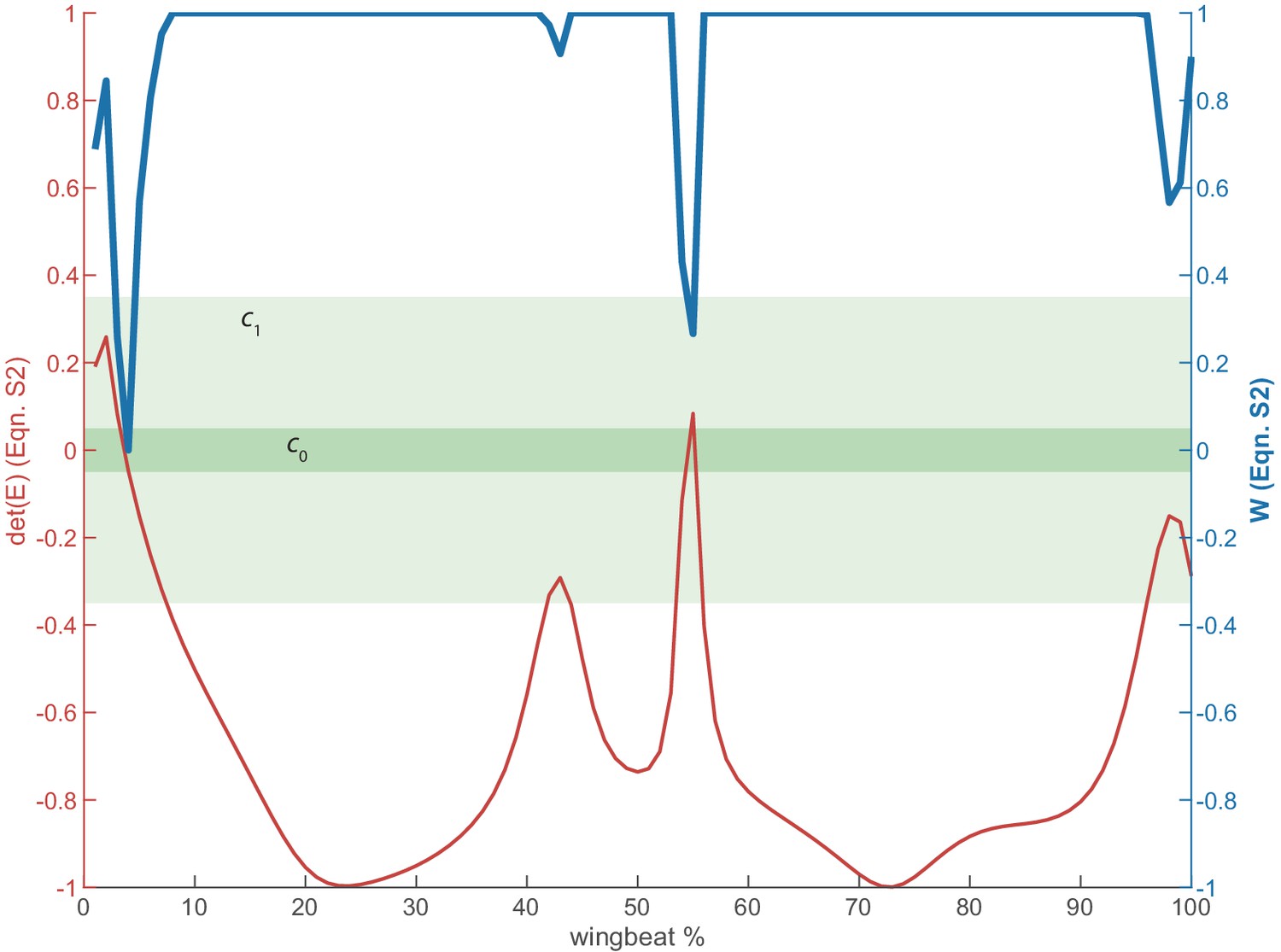
Illustration of regularization for lift and drag.
The lift and drag computations (Equation. A2) are sensitive when (red) is near zero, which occurs near stroke reversal. To temper the effects of these spikes, we apply a weight (blue) defined by Equation A6. When is in the dark green region, it is assigned a weight of zero. When is in the light green region, it is assigned a weight between zero and one. All other data in the white region are assigned a weight of one.
Figure 2—figure supplement 4
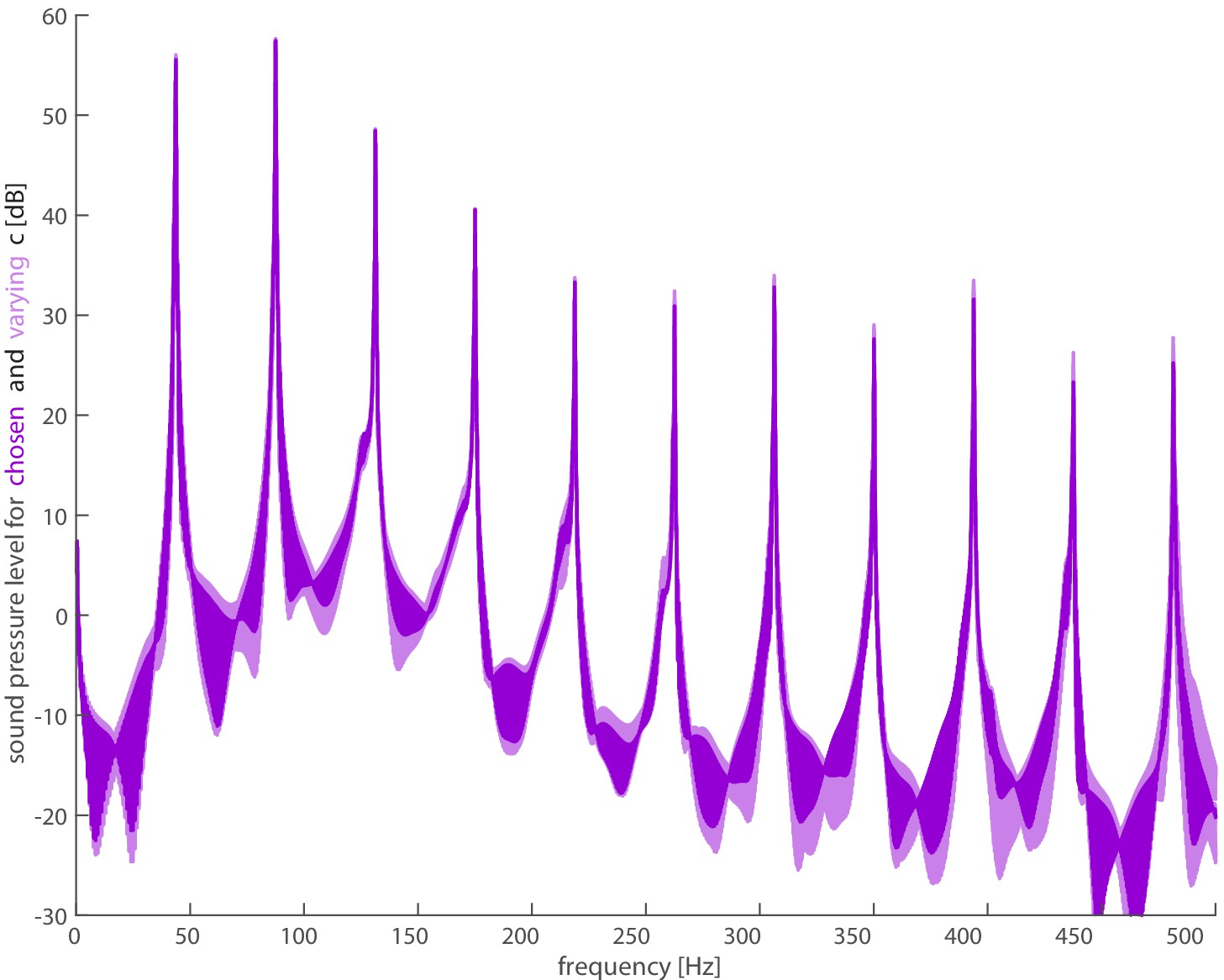
Choice of regularization constants does not appreciably affect smoothing.
The lift and drag forces are inputs to the full acoustic model, but need to be regularized due to sensitivities near stroke reversal. We varied the regularization constants of from 0.01 to 0.1 and from 0.2 to 0.5 (light purple), and we did not find substantial differences in the resultant spectra. We used the reported values of and (dark purple) from Chin and Lentink, 2019.
Figure 2—figure supplement 5
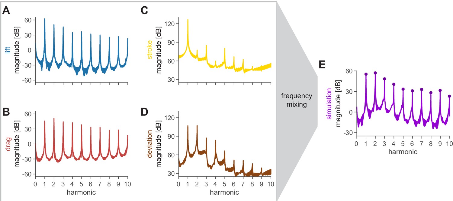
Spectra of all inputs into the acoustic model reveal the source of humming harmonics and evidence of frequency mixing.
(A and B) The lift and drag profiles were obtained from the kinematic (filtered at 400 Hz) and force (filtered at 180 Hz) data. The synthesis of these data results in the first stage of frequency mixing, whereby there is relatively high power even into higher harmonics. (C and D) The stroke and deviation define the position of the acoustic source and were obtained from the kinematic data. These spectra decay faster at higher harmonics. (E) The simulation spectra exhibit a mixture of the behavior of the inputs, with prominent peaks similar to the lift and drag forces (A and B), and a decay similar to the kinematics (C and D).
Figure 2—figure supplement 6
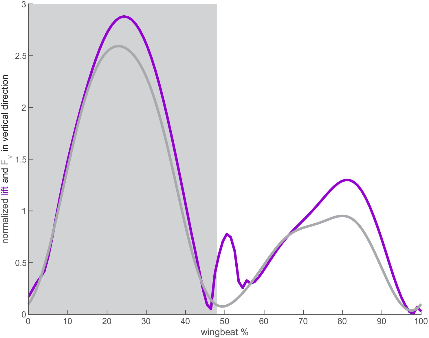
Agreement between calculated lift and weight support in the vertical direction.
The calculated lift (purple) for both wings in the vertical direction agrees well with the vertical weight support in the vertical direction (gray) as measured by Ingersoll and Lentink, 2018.
Figure 2—figure supplement 7
Sensitivity of the spectrum to the location of the acoustic point force along the wing radius.
The spectrum for the full acoustic model does not change appreciably when the source is located at (chosen value; purple), (gray), or (gray). Note that the plots overlap, so differences at the different harmonics can be viewed in Supplementary file 4.
Figure 3 with 1 supplement
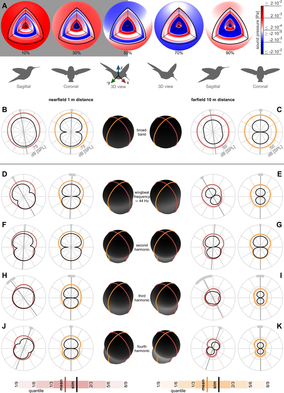
Nearfield versus farfield measured radial sound pressure level generated by a hovering hummingbird.
(A) The full 3D broadband (from 3 to 500 Hz; animated in Video 1) pressure field measured over a wingbeat from bird #1 (oriented as the 3D view avatar) is shown across the spherical circumference at 1 m radius, the acoustic nearfield (outside the wing radius of the bird, 8 cm) and at 10 m radius, the acoustic farfield (wavelength of first wingbeat harmonic is 7.8 m). These 3D acoustic field reconstructions are based on the measurements from all arrays (Figure 1D). (B) At a nearfield distance of 1 m, the 3D broadband pressure surfaces can be represented with cross sections along the two key anatomical planes, the side/sagittal and front/coronal plane respectively, to visualize the broadband pressure directivity over the entire wingbeat. The mean pressure directivity trace for all birds is colored dark with color coding referring to the anatomical plane, the quantiles for each of the six birds are shaded light, and model prediction are shown in black. The overall pressure shape in 3D is plotted in the middle in black, which has a roughly spherical shape in the broadband holograms. (C) The 3D broadband pressure directivity at a farfield distance of 10 m. The waists of the individual lobes in each flight are smeared out due to small variations between the birds and their flights, obscuring the directivity in the average plots (individual traces shown in Figure 3—figure supplement 1). To show where the principle axes of the individual pressure lobes fall, we calculated the waistline pressure level between the minimum lobes and plot the directivity axis as the line perpendicular to the waistline (gray line, light gray arc ±1 SD; D, E). The broadband hologram can be further decomposed into contributions from the first harmonic. The measurement and simulations match better for the nearfield (computationally backpropagated) than for the farfield (computationally propagated). In the sagittal plane, the dipoles for both the measurement and model are tilted aft. This tilt can also be observed as a rotational mode associated with the wingbeat frequency in the longitudinal direction in the 3D animation for the first harmonic for bird #1 (Video 2). In contrast, the associated coronal dipoles are oriented vertical. The 3D pressure shape is also more oblong, as viewed by the ovoid black shape in the middle. (F, G) The sagittal and coronal dipoles of the second harmonic are oriented vertically in both the nearfield and farfield. This vertical orientation is associated with the vertical force generation occurring twice per wingbeat and is also visible in the 3D animation for the second harmonic (Video 3). (H, I) We observed a rotational mode in the 3D animation for the third harmonic (Video 4). (J, K) Both the sagittal and coronal dipoles of the fourth harmonic are oriented vertical in both the nearfield and farfield, which is also visible in the animation (Video 5). The third and fourth harmonic are decompositions of the first two modes; therefore, they share directivity similarities. Finally, the data driven model prediction in B-K (black contours) match the in vivo data reasonably well in amplitude considering the differences in peak spectrum amplitude noted in Table 1. There is also good agreement in the directivity of the predicted angles for the first two harmonics for both sagittal and coronal planes and for the first four harmonics for the coronal plane (Table 2), which matches the agreement in amplitude.
Figure 3—figure supplement 1
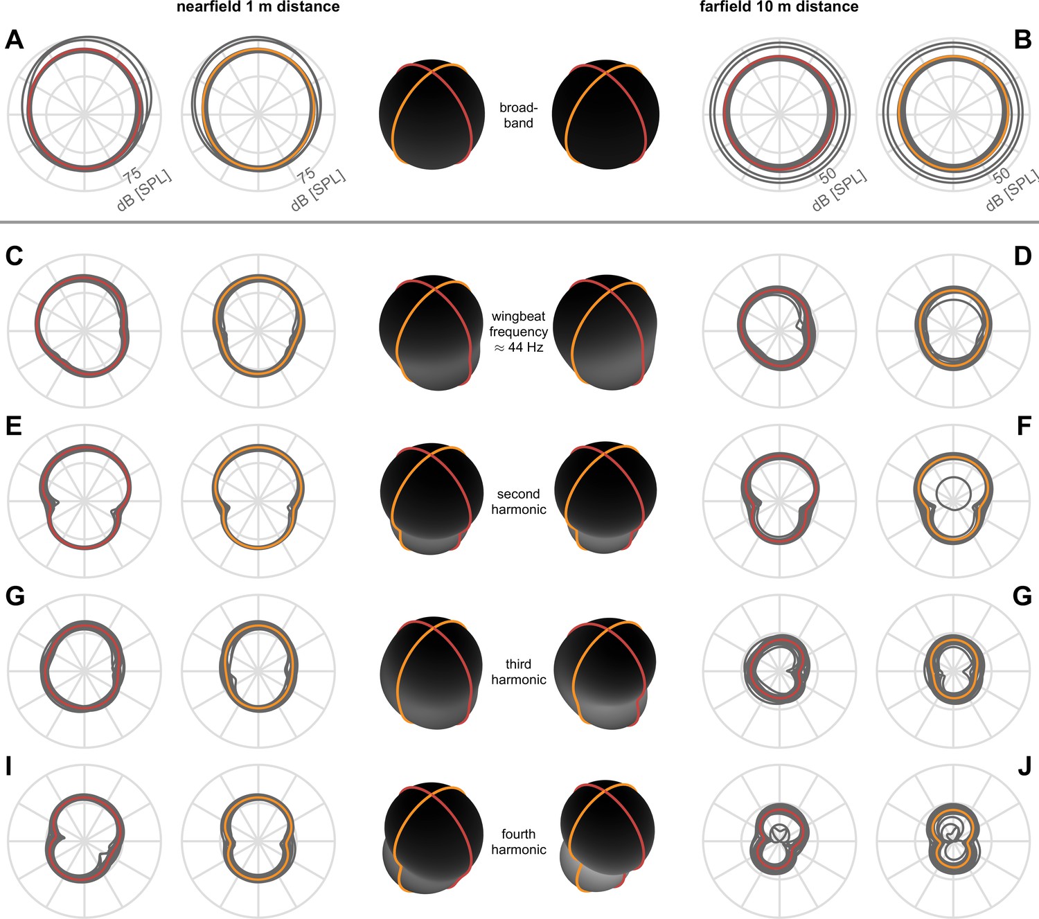
Individual directivity traces show waistlines.
The principal axis of each dipole is oriented perpendicular to the waistline (narrow region). The waistlines of individual lobes in each flight are smeared out due to small variations (in orientation, wingbeat, position, etc.) between birds and between flights of the same bird. Individual directivity measurements are shown in gray, and the averages are shown in red for sagittal and orange for coronal planes.
Figure 4 with 2 supplements
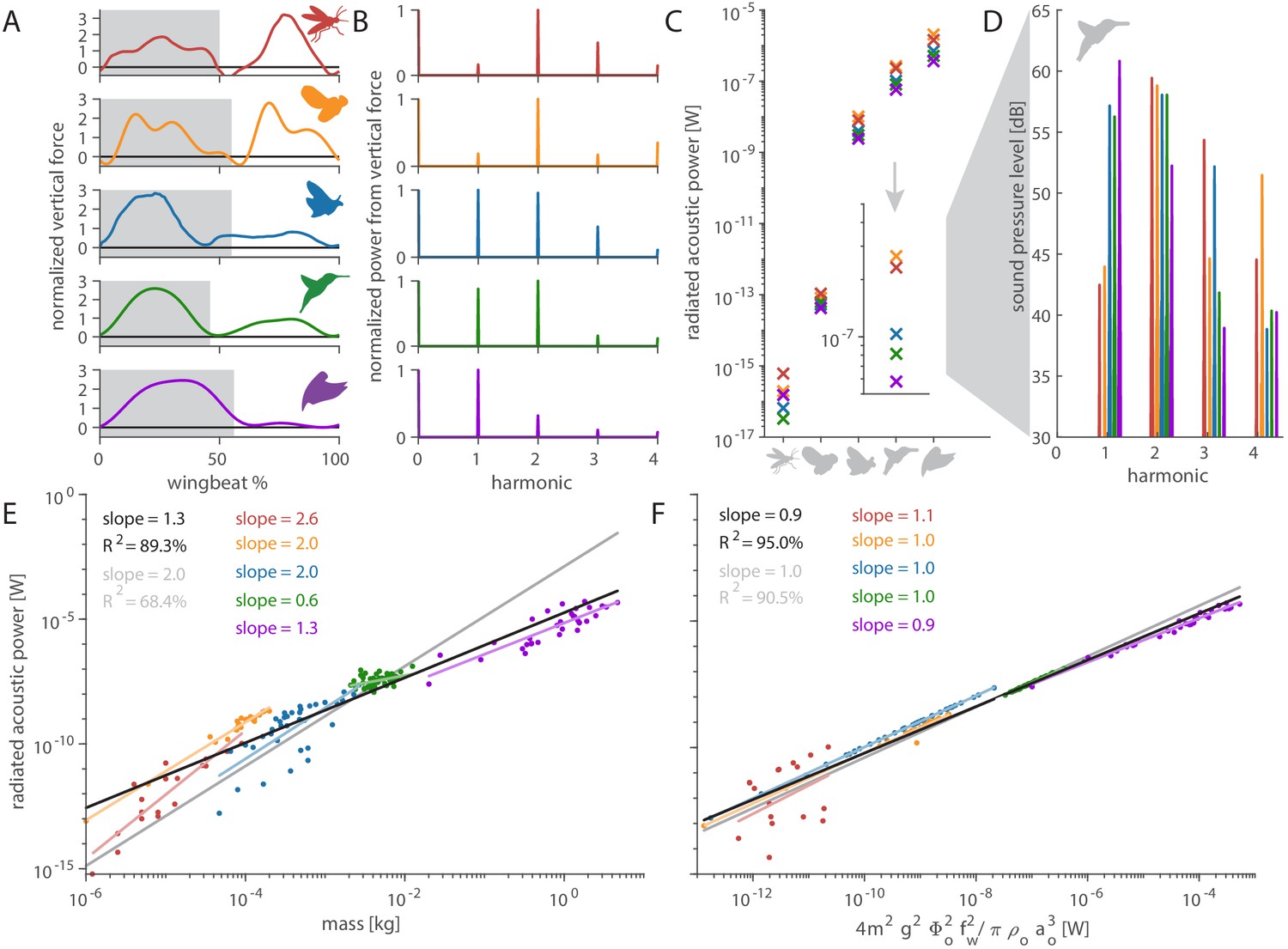
Distinct aerodynamic weight support profiles and non-allometric flapping wing scaling differentiates the acoustic spectrum and radiated power of flapping wing hum.
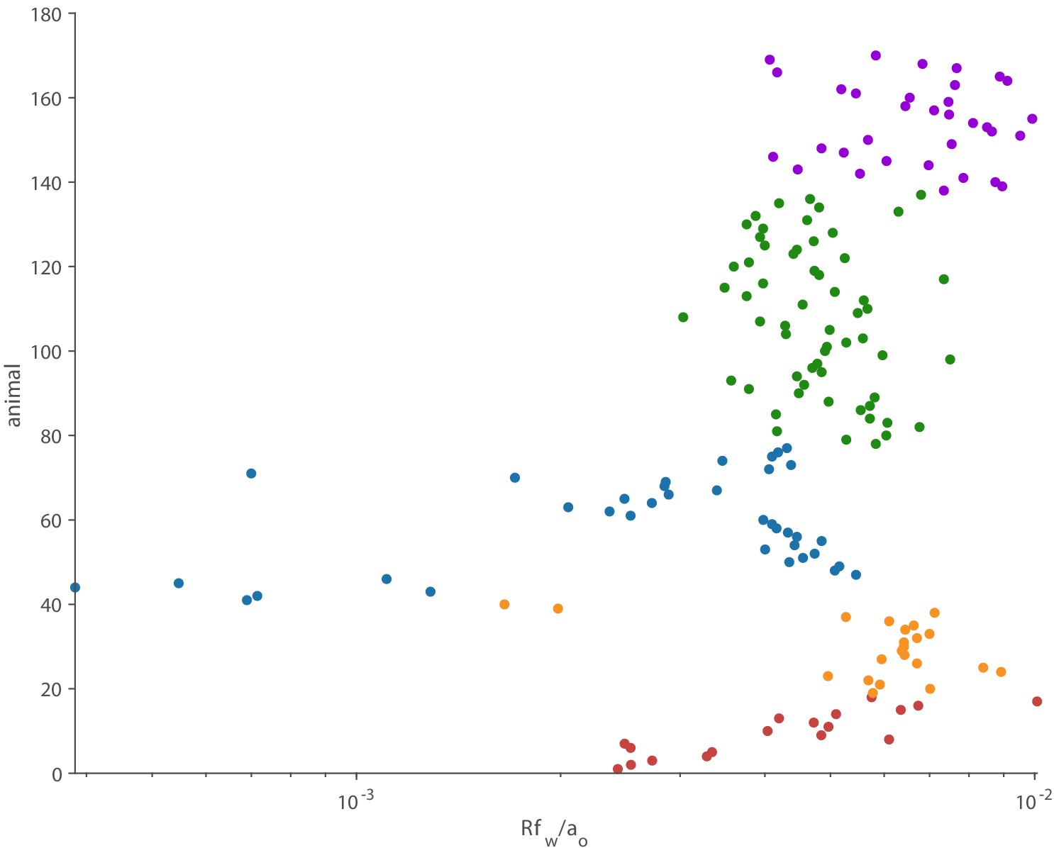
(A) Representative aerodynamic weight support profiles of paradigm animals representing elongated flies, compact flies, butterflies and moths, hummingbirds, and generalist birds. The representative weight support profile was used to simulate the hum across animals in each group, with body mass varying over seven orders of magnitude and flapping frequency over three orders of magnitude. (B) The frequency content of these weight support profiles is distinct. Elongated flies and compact flies concentrate energy at the second harmonic and have substantial frequency content at higher harmonics compared to hummingbirds and hawkmoths, which have high first and second harmonics. In contrast, parrotlets concentrate most of their energy at the first harmonic. (C) Using our aeroacoustics model, we prescribed each of the five animals (gray avatars) all five weight support profiles (red, orange, blue, green, and purple datapoints match avatars in A) to determine how this affected the total radiated acoustic power of the wing hum (e.g. a fly was prescribed the respective weight support profiles of a mosquito, fly, hawkmoth, hummingbird, and parrotlet). The weight support profiles of the mosquito and fly consistently generate more radiated power than the profiles of the other animals. Differences between the paradigm animal groups across the different scales are primarily governed by nonlinear interactions between the acoustic parameters. The inset zooms in on the model results at hummingbird scale, which reveals the marked influence of weight support profile on radiated power over one order of magnitude. (D) At the hummingbird scale, the weight support profiles (A and B) differentiate between the overall decibel level and distribution across the first four harmonics (to enhance readability we slightly shifted each spectrum from the harmonic to the left). (E) We find these effects across the seven orders of magnitude across which body mass ranges for the 170 flying animals that perform flapping flight. The model is based on body mass, wing length, and flapping frequency of each individual species combined with the weight support profile of the associated paradigm animal (A). The computational results across all species (black line, best-fit scaling across all groups) show the simplified scaling law derived from the acoustic equations used in the model (gray line, predicted scaling result) closely matches the computational outcome for moths and butterflies (blue line). Other groups deviate appreciably from the acoustic scaling law prediction (colored lines, best-fit scaling per group), because their wing length and flapping frequency scale allometrically with body mass. (F) To test if the acoustic scaling law is reasonably accurate for all groups when allometric scaling is incorporated, we plot the simulated radiated acoustic power versus the scaling law: the product of force, stroke amplitude and flapping frequency squared (divided by the constant product of air density and speed of sound). On average this shows good agreement between the computational model (black line) and scaling law prediction (gray line) across all groups.
Figure 4—figure supplement 1
The multiplicative factor is much smaller than one for all 170 animals.
At the wingbeat frequency, all these animals act as compact acoustic sources.
Figure 4—figure supplement 2

The flapping Mach number is small for all 170 animals.
This value is below 0.3, so the flow can be treated as subsonic.
Videos
Video 1
The 3D broadband hologram shows how pressure waves emanate from the nearfield to farfield.
Video 2
The 3D hologram for the first harmonic conveys the rotational mode associated with the tilted dipole.
Video 3
The 3D hologram for the second harmonic conveys the vertical mode associated with the vertically oriented dipole.
Video 4
The 3D hologram for the third harmonic conveys the rotational mode associated with the tilted dipole.
Video 5
The 3D hologram for the fourth harmonic conveys the vertical mode associated with the vertically oriented dipole.
Tables
Table 1
The measured and predicted sound pressure level peaks across the first 10 harmonics.
The measurement and model are close up to the fourth harmonic. The over-prediction for the seventh harmonic and up may be attributed to frequency mixing. Past the tenth harmonic, we approach the ambient noise floor for the measurements.
| Harmonic | 1st | 2nd | 3rd | 4th | 5th | 6th | 7th | 8th | 9th | 10th |
|---|---|---|---|---|---|---|---|---|---|---|
| Measurement [dB] ± SD [dB] | 60.8 ±1.2 | 60.0 ±1.2 | 47.9 ±2.6 | 46.4 ±3.4 | 42.7 ±3.2 | 41.7 ±3.2 | 34.0 ±2.6 | 28.8 ±3.7 | 23.6 ±3.1 | 25.2 ±2.3 |
| Model [dB] | 55.3 | 57.0 | 48.4 | 40.5 | 33.4 | 30.9 | 32.9 | 28.1 | 31.5 | 23.1 |
Table 2
The measured and predicted broadband pressure directivity angles match.
Aft tilt is evident in the sagittal planes, whereas the coronal planes show vertical directionality associated with vertical force generation. Harmonic modes 1–4 match well in the coronal plane and modes 1 and 2 match well in the sagittal plane.
| Broadband | Sag near | Cor near | Sag far | Cor far |
|---|---|---|---|---|
| Measurement [°] ± SD [°] | 99.4 ±3.1 | 88.0 ±3.4 | 97.4 ±3.2 | 89.1 ±4.6 |
| Model [°] | 102.3 | 90.2 | 97.8 | 90.0 |
| Sagittal nearfield | 1st | 2nd | 3rd | 4th |
| Measurement [°] ± SD [°] | 119.7 ±3.4 | 86.3 ±1.9 | 126.9 ±13.7 | 69.6 ±5.0 |
| Model [°] | 125.8 | 99.8 | 82.7 | 44.3 |
| Sagittal Farfield | 1st | 2nd | 3rd | 4th |
| Measurement [°] ± SD [°] | 120.4 ±4.4 | 85.4 ±2.2 | 116.6 ±24.4 | 70.8 ±5.1 |
| Model [°] | 125.6 | 99.8 | 78.9 | 44.6 |
| Coronal nearfield | 1st | 2nd | 3rd | 4th |
| Measurement [°] ± SD [°] | 86.7 ±8.8 | 89.7 ±2.7 | 88.7 ±9.3 | 89.8 ±4.1 |
| Model [°] | 89.9 | 90.2 | 89.9 | 90.0 |
| Coronal Farfield | 1st | 2nd | 3rd | 4th |
| Measurement [°] ± SD [°] | 89.4 ±6.6 | 90.2 ±2.8 | 90.5 ±10.3 | 90.9 ±7.2 |
| Model [°] | 90.1 | 90.0 | 90.0 | 90.0 |
Additional files
-
Supplementary file 1
Summary of the number of acoustic measurements made for each bird.
To obtain frequency resolution ≤ 2 Hz, we selected feeding flights of 0.5 s or longer.
- https://cdn.elifesciences.org/articles/63107/elife-63107-supp1-v2.docx
-
Supplementary file 2
Comparison between the 10-element distributed source model and equivalent point source model.
To investigate how well hummingbird flapping wing hum can be approximated with a single acoustic source per wing, we created a distributed oscillating source model with ten equally spaced elements along each wing. The force distribution was adapted from a high-fidelity model by Ingersoll and Lentink, 2018 for the same hummingbird species. There is close agreement in magnitude for the first ten harmonics of the single and ten source model.
- https://cdn.elifesciences.org/articles/63107/elife-63107-supp2-v2.docx
-
Supplementary file 3
Comparison between the full and simplified acoustic models.
There is reasonable agreement in magnitude for the first four harmonics.
- https://cdn.elifesciences.org/articles/63107/elife-63107-supp3-v2.docx
-
Supplementary file 4
Comparison between the different acoustic source locations.
When the acoustic source is located at (chosen), , or , the resultant spectra have similar peak magnitudes.
- https://cdn.elifesciences.org/articles/63107/elife-63107-supp4-v2.docx
-
Supplementary file 5
Summary of values used for paradigm animals in acoustic models.
Culex quinquefasciatus was adapted from Bomphrey et al., 2017. Drosophila hydei mass was adapted from Greenewalt, 1962, while the other parameters were adapted from Muijres et al., 2014. Manduca sexta parameters were adapted from Zheng et al., 2013. Calypte anna values were obtained from the present experiment. Forpus coelestis values were adapted from Chin and Lentink, 2017. To simplify the comparison between the five paradigm animals, we approximated the stroke plane as horizontal and the normalized lift profile to have the same shape as the reported vertically oriented force profile (‘Normalized Lift Profile Proxy’), so that the lift generated during a wingbeat summed up to body weight for all associated species in the same way. ** and ***: these forces do not equate to lift, but we used the normalized profile as an approximation for the lift profile. * and ***: these forces do not necessarily equate to body weight when integrated over a wingbeat in hover. **: these forces do equate to body weight when integrated over a wingbeat in hover. * and ** and ***: the normalized profiles of these forces were used and either equate to or are a proxy for the lift profiles.
- https://cdn.elifesciences.org/articles/63107/elife-63107-supp5-v2.docx
-
Transparent reporting form
- https://cdn.elifesciences.org/articles/63107/elife-63107-transrepform-v2.docx
Download links
A two-part list of links to download the article, or parts of the article, in various formats.
Downloads (link to download the article as PDF)
Open citations (links to open the citations from this article in various online reference manager services)
Cite this article (links to download the citations from this article in formats compatible with various reference manager tools)
How oscillating aerodynamic forces explain the timbre of the hummingbird’s hum and other animals in flapping flight
eLife 10:e63107.
https://doi.org/10.7554/eLife.63107


