Spherical arena reveals optokinetic response tuning to stimulus location, size, and frequency across entire visual field of larval zebrafish
- University of Tübingen, Werner Reichardt Centre for Integrative Neuroscience and Institute of Neurobiology, Germany
- Sussex Neuroscience, School of Life Sciences, University of Sussex, United Kingdom
Figures
Figure 1 with 2 supplements
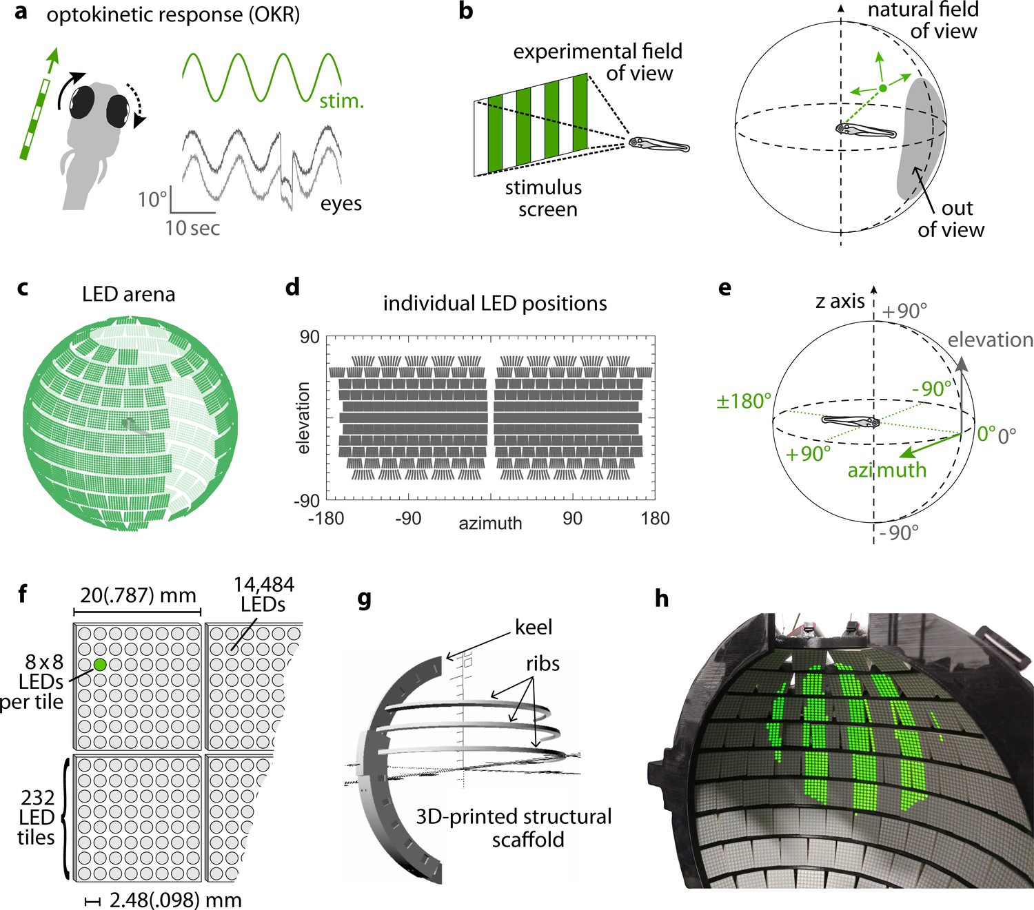
Presenting visual stimuli across the visual field.
(a) When presented with a horizontal moving stimulus pattern, zebrafish larvae exhibit optokinetic response (OKR) behaviour, where eye movements track stimulus motion to minimise retinal slip. Its slow phase is interrupted by intermittent saccades, and even if only one eye is stimulated (solid arrow), the contralateral eye is indirectly yoked to move along (dashed arrow). (b) Often, experiments on visuomotor behaviour such as OKR sample only a small part of the visual field, whether horizontally or vertically. As different spatial directions may carry different behavioural importance, an ideal stimulation setup should cover all or most of the animal’s visual field. For zebrafish larvae, this visual field can be represented by an almost complete unit sphere. (c) We arranged 232 LED tiles with 64 LEDs each across a spherical arena, such that 14,484 LEDs (green dots) covered nearly the entire visual field. (d) The same individual positions, shown in geographic coordinates. Each circle represents a single LED. Each cohesive group of eight-by-eight circles corresponds to the 64 LEDs contained in a single tile. (e) To identify LED and stimulus locations, we use Up-East-North geographic coordinates: Azimuth describes the horizontal angle, which is zero in front of the animal and, when seen from above, increases for rightward position. Elevation refers to the vertical angle, which is zero throughout the plane containing the animal, and positive above. (f) The spherical arena is covered in flat square tiles carrying 64 green LEDs each. (g) Its structural backbone is made of a 3D-printed keel and ribs. Left and right hemispheres were constructed as separate units. (h) Across 85-90% of the visual field, we can then present horizontally moving bar patterns of different location, frequency and size to evoke OKR.
-
Figure 1—source data 1
SCAD files for 3D-printing the arena scaffold.
- https://cdn.elifesciences.org/articles/63355/elife-63355-fig1-data1-v2.zip
Figure 1—figure supplement 1

A spherical LED arena to present visual stimuli across the visual field.
(a) LED tiles are arranged in ribbons parallel to the equator and glued in between structural ribs. Gaps at the top and bottom pole of the sphere allow coupling in an optical pathway for infrared illumination and subsequent video recording of eye movement. The fish is placed at the centre of the sphere, facing the observer. See the Supplementary file 1A as well as the mathematical manual in our data repository for more on the angles . (b) Optical pathway for eye movement tracking. (c) To minimise obstruction and refraction, the zebrafish larva is immobilised on the tip of a glass triangle (left) using agarose, which is then inserted into the centre of a spherical glass bulb (middle). This bulb is then mounted into a metal holder (right) and thus placed at the centre of the sphere. (d) Image of the two hemispheres and the camera setup. One hemisphere is mounted on a rail to allow opening and closing the arena.
Figure 1—figure supplement 2
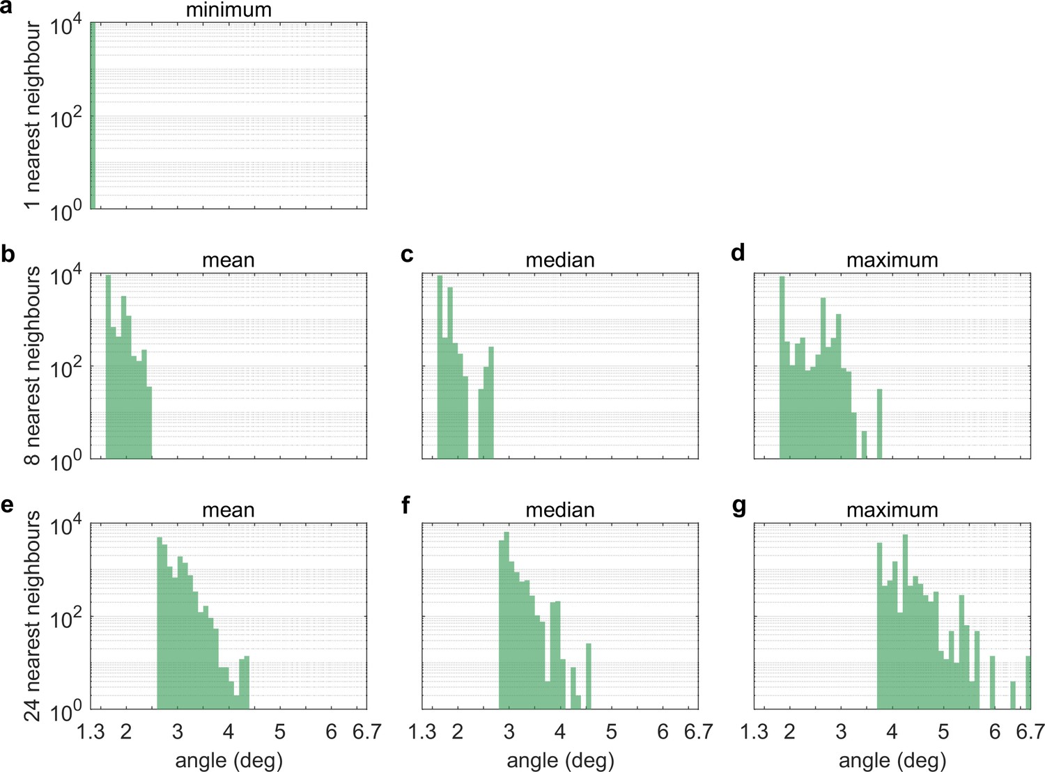
Nearest-neighbour distances between LEDs.
Histograms of (a) the angle between an LED and its nearest neighbour, (b) the mean, (c) median and (d) maximum angle between an LED and its eight nearest neighbours, and (e) the mean, (f) median and (g) maximum angle between an LED and its 24 nearest neigbours. Whereas (a) only captures the microstructure of LED tiles, where 8 by 8 LED are arranged in a square pattern, (b-d) and especially (e-g) also capture edge effects and gaps in between tiles.
Figure 2 with 2 supplements

OKR gain is inferred from a piece-wise fit to the slow phase of tracked eye movements.
(a) We present a single pattern of horizontally moving bars to evoke OKR and crop it by superimposing a permanently dark area of arbitrary size and shape (left). Its velocity follows a sinusoidal time course, repeating every 10 s for a total of 100 s for each stimulus phase (right). (b) OKR gain is the amplitude of eye movement (green trace) relative to the amplitude of the sinusoidal stimulus (grey trace). The OKR gain is often well below 1, e.g. for high stimulus velocities as used here (up to 12.5°/s). (c) Even small stimuli are sufficient to elicit reliable OKR, although gains are low if stimuli appear in a disfavoured part of the visual field. Shown here are responses to a whole-field stimulus (top) and to a disk-shaped stimulus in the extreme upper rear (bottom, Figure 2—figure supplement 2).
Figure 2—figure supplement 1
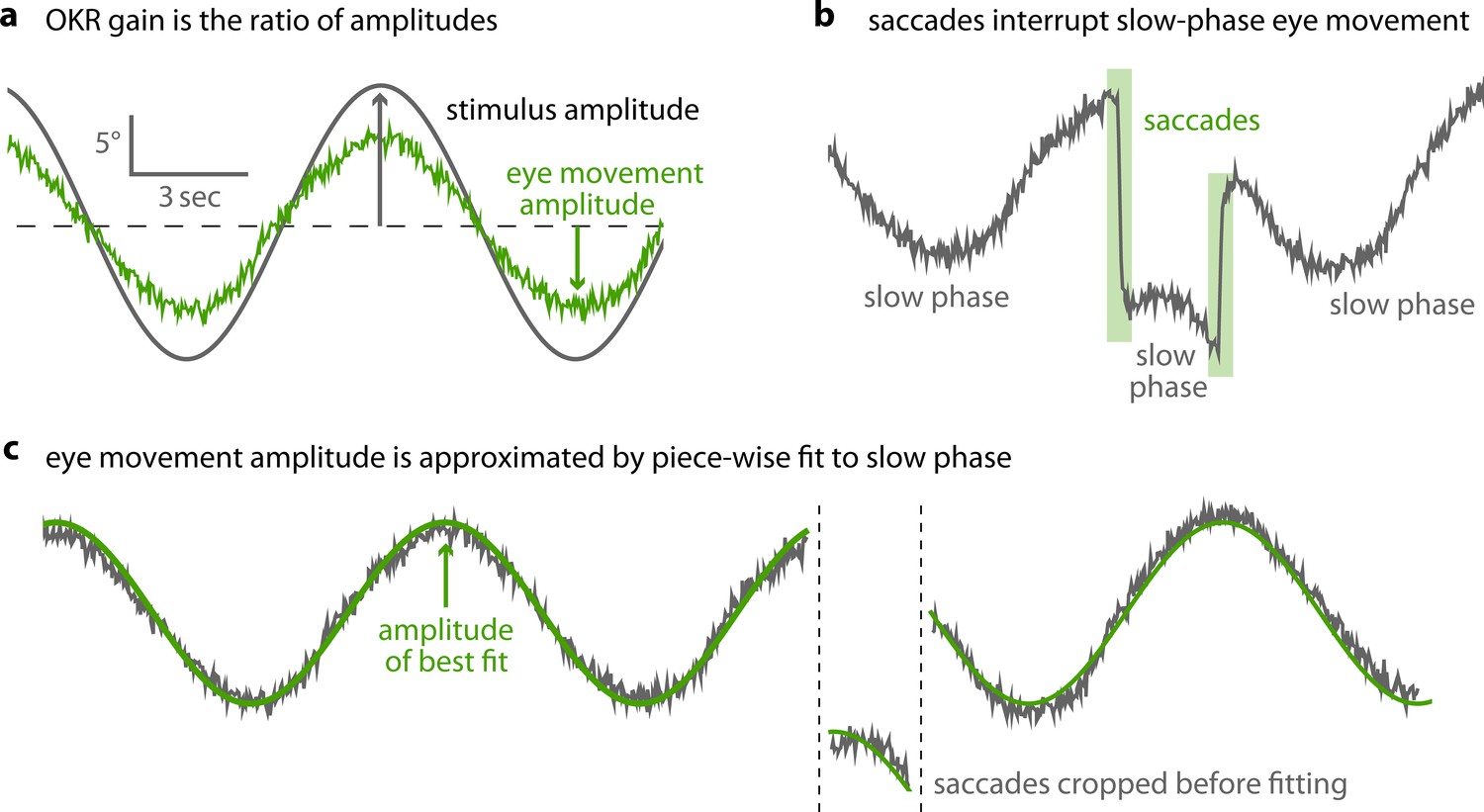
Saccades are cropped before OKR gain is measured.
(a) As shown in Figure 2b, optokinetic gain is the ratio between the amplitudes of eye movement and stimulus movement. To extract these, raw eye traces must be processed. (b) OKR eye movements consist of a slow phase, gradually tracking stimulus motion, and intermittent saccades. (c) After pre-processing data to detect and remove saccades, we fit a piece-wise sinusoidal function with a single amplitude to the remaining slow-phase eye traces. The amplitude of the best fit determines OKR gain.
Figure 2—figure supplement 2
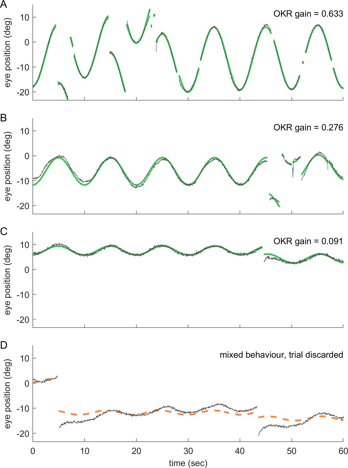
Even at remote stimulus locations, fish exhibit reliable OKR behaviour; trials with mixed behaviour are excluded.
(a–d) show 60 s samples of eye position traces obtained during visual stimulation (dark grey traces). Saccades were cropped, as demonstrated in Figure 2—figure supplement 1. Positive angles correspond to more rightward eye positions. Coloured traces show best fit to data (see Materials and methods), along with the resulting OKR gain. Fish were presented with either (a) whole field visual stimuli, or (b–d) smaller disk-shaped stimuli, as in Figure 3. (a) Whole-field stimulation elicits reliable OKR, even though high stimulus frequencies keep its gain below 1. (b) The same is true for disk stimulus in a preferred region of the visual space (stimulus D7, azimuth −90°, elevation +39°, that is lateral and dorsal to the fish), although the smaller stimulus evokes a smaller OKR gain. (c) Disk stimuli presented in a disfavoured part of the visual field (stimulus D3, azimuth −90°, elevation +74°, almost dorsal to the fish) evoke significantly lower gains, but still reliable OKR behaviour. Data in (a,c) correspond to trials shown in Figure 2c. (d) As it is possible to encounter behaviours other than OKR, or in addition to OKR, we inspected all trials before data analysis. Trials in which no pure OKR was present, such as the one shown here, were excluded (stimulus D3, same as in c).
Figure 3 with 6 supplements
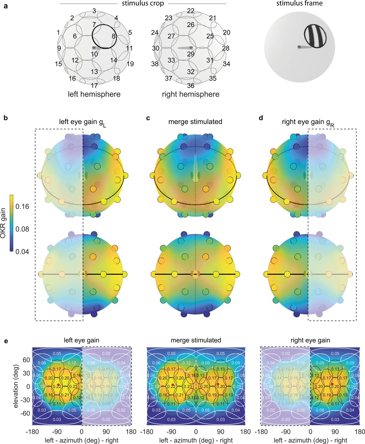
OKR gain depends on stimulus location.
(a) The stimulus is cropped to a disk-shaped area 40 degrees in diameter, centred on one of 38 nearly equidistant locations (Supplementary file 1B) across the entire visual field (left), to yield 38 individual stimuli (right). (b–d) Dots reveal the location of stimulus centres D1-D38. Their colour indicates the average OKR gain across individuals and trials, corrected for external asymmetries. Surface colour of the sphere displays the discretely sampled OKR data filtered with a von Mises-Fisher kernel, in a logarithmic colour scale. Top row: OKR gain of the left eye (b), right eye (d), and the merged data including only direct stimulation of either eye (c), shown from an oblique, rostrodorsal angle. Bottom row: same, but shown directly from the front. OKR gain is significantly higher for lateral stimulus locations and lower across the rest of the visual field. The spatial distribution of OKR gains is well explained by the bimodal sum of two von-Mises Fisher distributions. (e) Mercator projections of OKR gain data shown in panels (b–d). White and grey outlines indicate the area covered by each stimulus type. Numbers indicate average gain values for stimuli centred on this location. Red dots show mean eye position during stimulation. Dashed outline and white shading on panels (b, d, e) indicate indirect stimulation via yoking, that is, stimuli not directly visible to either the left or right eye. Data from n = 7 fish for the original configuration and n = 5 fish for the rotated arena.
-
Figure 3—source data 1
Numerical data and graphical elements of Figure 3b–d.
- https://cdn.elifesciences.org/articles/63355/elife-63355-fig3-data1-v2.mat
-
Figure 3—source data 2
Numerical data and graphical elements of Figure 3e.
- https://cdn.elifesciences.org/articles/63355/elife-63355-fig3-data2-v2.mat
Figure 3—figure supplement 1
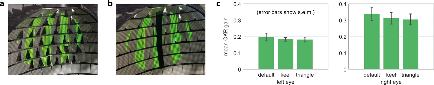
Gaps in the arena do not bias OKR behaviour.
(a) Artificial triangular holes setup. (b) Artificial keel setup. (c) Neither triangular nor elongated gaps result in significantly different OKR gains (n = 5 fish).
Figure 3—figure supplement 2

During OKR, the beating field and average eye position are independent of stimulus location.
All data were pooled across fish and trials. One gain value was computed per stimulus presentation. Violin plots show distribution of mean horizontal eye positions across the pooled data; vertical lines indicate 25th percentile, median and 75th percentile of the distribution. Positions are those during presentation of stimulus types (a) D1 to D38 shown in Figure 3a, (b) A1 to A42 shown in Figure 5b, (c) F1 to F42 shown in Figure 5a. Dashed lines in (c) represent axis limits of (a,b).
Figure 3—figure supplement 3
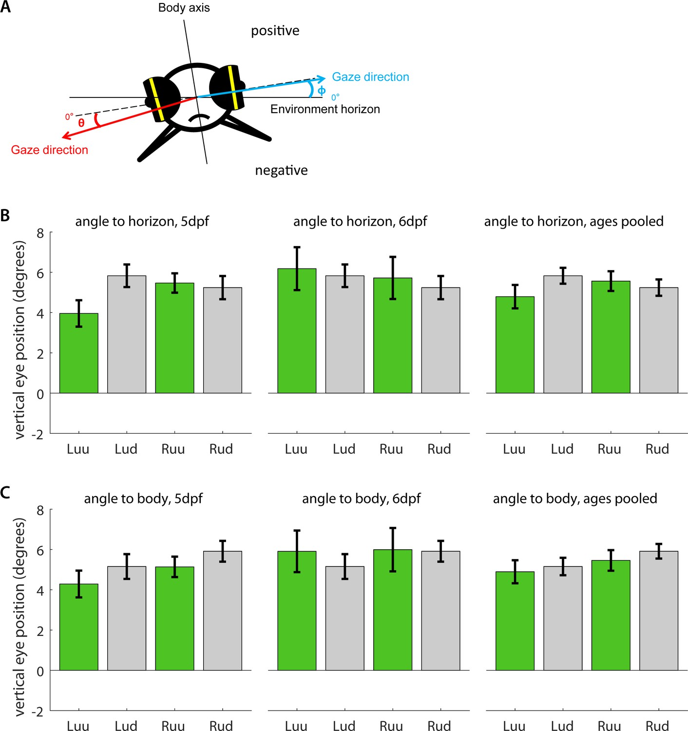
Vertical eye position under upright and upside-down embedding.
(a) Five dpf and six dpf larvae were embedded in agarose with their eyes cut free and placed under a microscope. Using an additional mirror, we recorded simultaneous image time series along both the dorsoventral and mediolateral axes. Vertical eye position was determined geometrically for each individual frame (see Materials and methods). Because some larvae were embedded in such a way that mediolateral axis was not entirely aligned with the true horizon of the environment, we measured vertical eye position (b) relative to both the true environmental horizon, and (c) the mediolateral body axis, and in both cases, compared the left (L) and right eyes (R) of larvae embedded upside-up (uu) or upside-down (ud). To facilitate comparison, positive signs were chosen to roughly correspond to the dorsal hemisphere in both cases. Bars indicate mean after pooling across all frames, error bars show corresponding standard error of the mean (s.e.m.). In summary, larval eyes were almost always inclined towards the dorsum, irrespective of the direction of embedding. The fish do not appear to compensate for their orientation with respect to the gravitational axis.
Figure 3—figure supplement 4
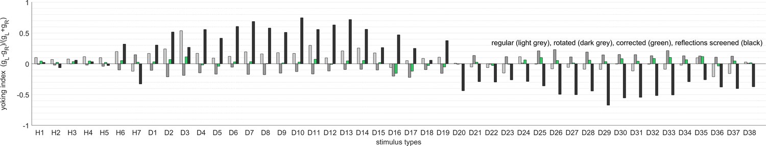
Yoking indices are biased by reflections within the arena.
Yoking indices were computed for experiments using the regular setup as in Figure 4a (light grey), with a rotated arena as in Figure 4b (dark grey), corrected for experimental asymmetries as in Figure 3 (green), and with one side of the glass bulb, contralateral to the stimulus centre, painted black (black). Yoking indices from most experiments are close to zero, indicating similar OKR gains for both eyes regardless of stimulus location. In contrast, yoking indices from the latter control experiment differ markedly from zero, indicating significantly weaker responses by the respectively unstimulated eye. This finding points to reflections at the air-glass interface being visible to the purportedly ‘unstimulated’ eye. Stimulus types are listed in the order given in Supplementary file 1B and Supplementary file 1E: the whole-field stimulus H1, hemifield stimuli H2 to H7, and then disk-shaped stimuli D1 to D38 from front to rear, top to bottom, and left hemisphere to right hemisphere.
Figure 3—figure supplement 5
Across different types of arenas, stimulus reflections affect perceived yoking.
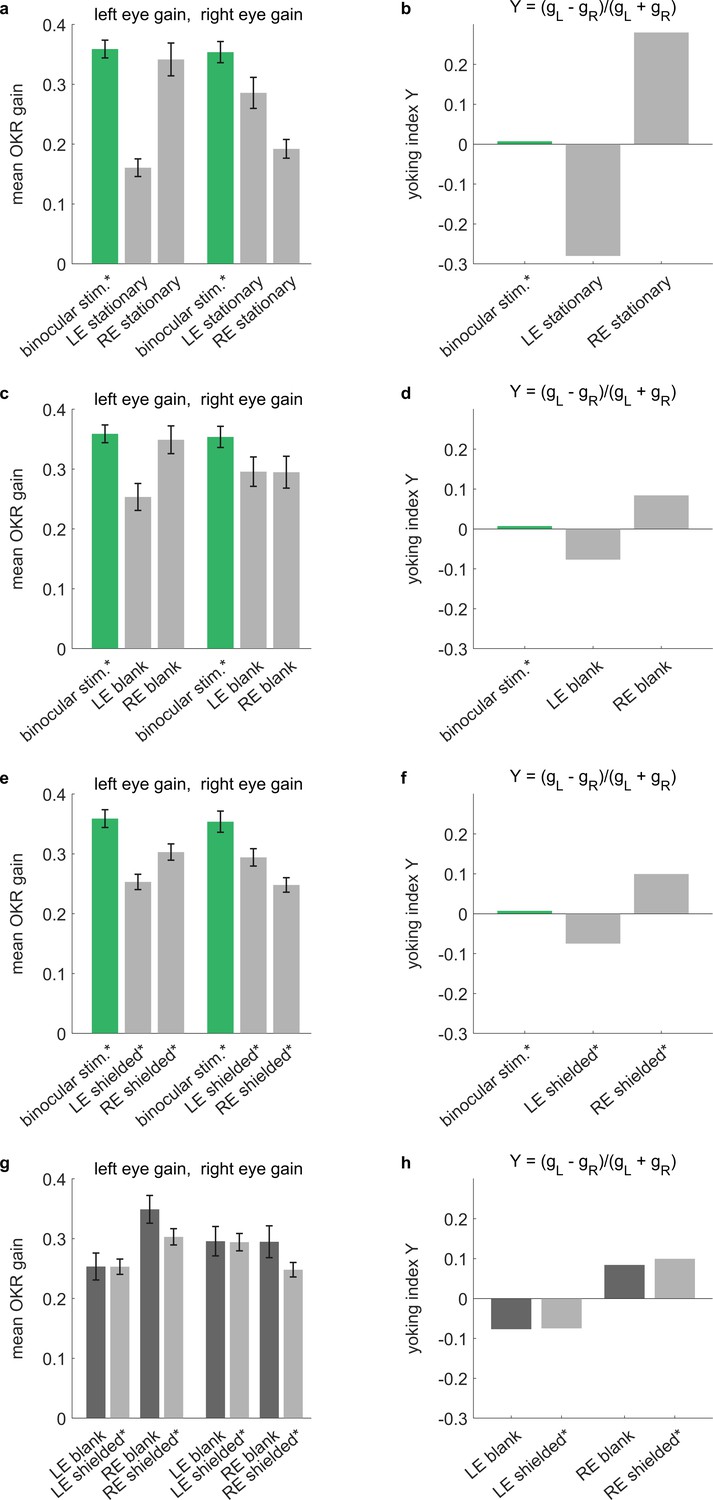
Control experiments conducted in a rectangular stimulus arena. OKR-inducing gratings were shown on all four stimulus screens surrounding the larvae, while additional elements were introduced around either the left eye (LE), the right eye (RE) or neither. Specifically, selected eyes were (a,b) shown stationary stimuli of the same frequency and contrast as the moving stimuli, (c,d) shown a blank white surface, or (e,f) shielded with a fully opaque cover. See Supplementary file 1D for an overview of stimulus combinations. (a,c,e,g) Bars indicate mean OKR gains, and error bars show standard error of the mean. (b,d,f,h) Yoking indices are near zero when both eyes move with identical amplitudes and positive when left eye amplitude exceeds that of the right eye (see Materials and methods). (a,b) In the presence of two conflicting stimuli (moving vs. stationary), yoking between the eyes is reduced by almost half, confirming that the unstimulated eye is yoked to the stimulated eye, albeit with a lower OKR gain. (c,d) When there is no conflicting stimulus, yoking drives OKR of the contralateral eyes, albeit with a lower amplitude as if both eyes were stimulated directly with identical stimulus, (e,f) which is equally true in the presence of shielding. (g,h) To assess the effect of reflections on the difference between directly stimulated and purportedly stimulated eyes, we compare blank stimuli (as in c-d, which could diffusely reflect light) to fully shielded eyes (as in e-f, where no reflections should occur). There are no significant differences, indicating that the larger effect of reflections observed in our spherical arena (Figure 3—figure supplement 4) may be caused by the different stimulus design or by different reflection properties. *Two rectangular arena setups were used for the control experiments. Asterisks indicate data obtained from the second setup, for which balanced illumination was explicitly confirmed via diode photodetector. Data from n = 22 fish for initial setup and n = 10 fish for second setup.
Figure 3—video 1
Animation showcasing short samples of all disk stimuli used to study location dependence, as in Figure 3a.
Figure 4 with 3 supplements

The OKR is biased towards upper environmental elevations irrespective of fish orientation.
(a) Regular arena setup. (b) Arena can be tilted 180 degrees so front and rear, upper and lower LED positions are swapped. The bulb holder moves accordingly, so from the perspective of the fish, left and right, upper and lower LEDs are swapped. (c) Upside-down embedding setup. (d) Setup with inverted optical path, including illumination. (e–h) Results in body-centred coordinates, where positive elevations refer to dorsal positions, for the four setups shown in (a–d). As in Figure 3b–e, colour indicates the discretely sampled OKR data filtered with a von Mises-Fisher kernel and follows a logarithmic colour scale. (g,h) Experiments with presentation of a less regularly distributed set of stimuli, cropped to disks of 64 degrees polar angle instead of the 40 degrees used in (a,b,e,f). (g) Fish embedded upside-down exhibit a slight preference for stimuli below the body-centred equator, that is, positions slightly ventral to their body axis. (h) Fish embedded upright, as in (a). To account for environmental asymmetries such as arena anisotropies, we combined the data underlying (e) and (f) to obtain Figure 3b–e (see Materials and methods). Data from (e) n = 7, (f) n = 5, (g) n = 3, (h) n = 10 fish.
-
Figure 4—source data 1
Numerical data and graphical elements of Figure 4e.
- https://cdn.elifesciences.org/articles/63355/elife-63355-fig4-data1-v2.mat
-
Figure 4—source data 2
Numerical data and graphical elements of Figure 4f.
- https://cdn.elifesciences.org/articles/63355/elife-63355-fig4-data2-v2.mat
-
Figure 4—source data 3
Numerical data and graphical elements of Figure 4g.
- https://cdn.elifesciences.org/articles/63355/elife-63355-fig4-data3-v2.mat
-
Figure 4—source data 4
Numerical data and graphical elements of Figure 4h.
- https://cdn.elifesciences.org/articles/63355/elife-63355-fig4-data4-v2.mat
Figure 4—figure supplement 1
Asymmetries between left and right eye are strongly affected by the environment.
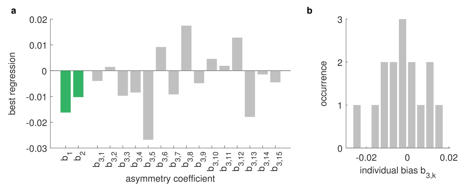
Differences between the OKR gains of directly stimulated left eyes and directly stimulated right eyes can be explained by a linear combination of biological and environmental factors, for example, biases of individual animals or asymmetries of the stimulus arena (see Materials and methods). Comparing data from the regular and rotated setups (Figure 4e–f), as well as data from fish immobilised upside-down (Figure 4g), including additional stimuli covering entire hemispheres (Supplementary file 1E), we can infer the underlying factors via multivariate regression of our linear model. We find that individual biases (grey) vary strongly from fish to fish and are broadly distributed from left to right. There are some constant biases across fish (green), both towards the left side of their visual field () and towards one of the two LED hemispheres (); however, these biases are small and, given the large variability of individual biases, might be a result of the limited number of fish studied. Underlying stimulus types are listed in Supplementary file 1B and Supplementary file 1E. (b) Histogram of individual-fish biases shows no collective preference for either side.
Figure 4—figure supplement 2
OKR gain maps for individual larvae.
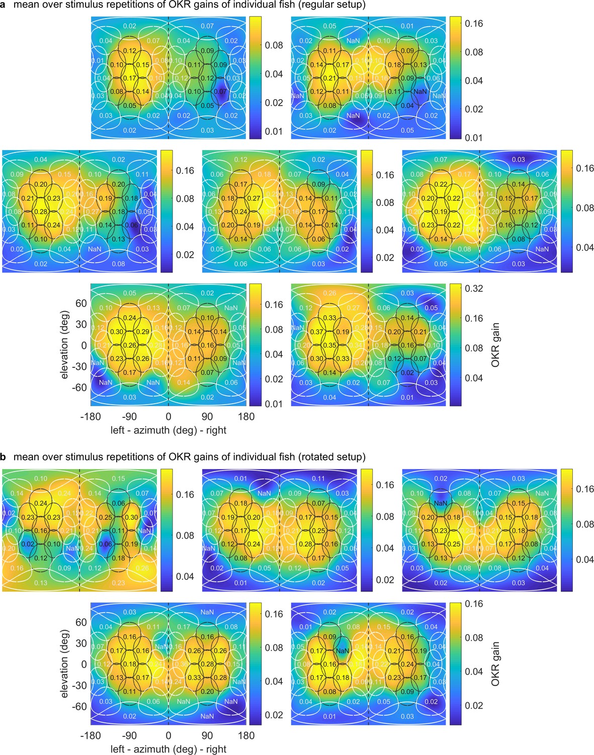
Mercator projections of OKR gain data as in Figure 3e and Figure 4e–h, but shown here for individual fish in (a) the regular setup, (b) the rotated arena. Data from n = 1 fish per panel. The results of the first fish in (b) are so irregular as to have likely been caused by experimenter error in preprocessing, rather than biologically meaningful differences. We thus excluded this fish from any analyses, such as the those for Figure 3 and Figure 4.
Figure 4—figure supplement 3
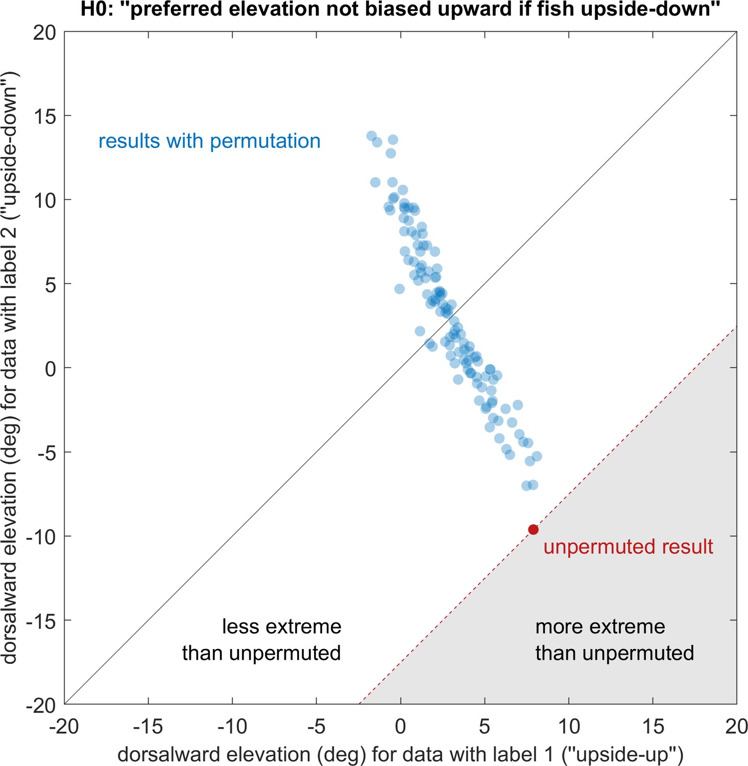
Elevation of stimuli evoking strongest OKR remains upward regardless of embedding direction.
See Materials and methods for a detailed description of the permutation test. Showing the actual observation (red) and all 119 non-redundant permutations (blue) that maintain relative group size, p<0.05. ‘Dorsalward’ refers to the dorsal hemisphere in a body-centred reference frame, as opposed to the ‘upper’ hemisphere in an environmental reference frame. Before permutation, label one corresponds to the experiments shown in Figure 4a, whereas label two corresponds to those in Figure 4c. The test statistic is the signed distance from the black diagonal, with results in the white area being less extreme than those of the unpermuted observation. The null-hypothesis is rejected, so the elevation of OKR gain peaks within the visual field is not determined in body-centred coordinates, but instead biased towards upper elevations (‘towards the sun’, world-centred coordinates).
Figure 5 with 5 supplements
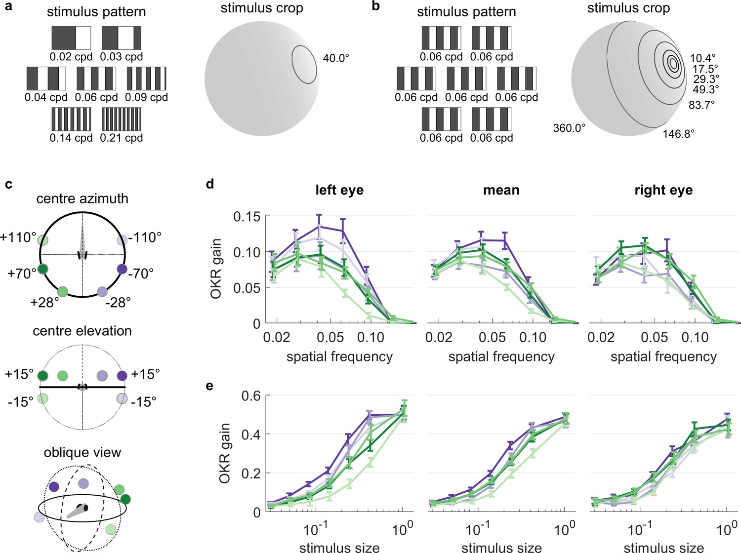
OKR tuning to spatial frequency is similar across different visual field locations.
(a) Patterns with seven different frequencies were cropped to disks of a single size. These disks were placed in six different locations for a total of 42 stimuli. cpd: cycles per degree. (b) Patterns with identical spatial frequencies were cropped to disks of seven different sizes. These disks were also placed in six different locations for another set of 42 stimuli. Degrees indicate planar angles subtended by the stimulus outline, so 360° correspond to whole-field stimulation. (a, b) Displaying the entire actual pattern at the size of this figure would make the individual bars hard to distinguish. We thus only show a zoomed-in version of the patterns in which 45 out of 360 degrees azimuth are shown. (c) Coloured dots indicate the six locations on which stimuli from a and b were centred, shown from above (top), from front (middle), and from an oblique angle (bottom). (d) OKR gain is unimodally tuned to a wide range of spatial frequency (measured in cycles per degree). (e) OKR gain increases sigmoidally as the area covered by the visual stimulus increases logarithmically (a stimulus size of 1 corresponds to 100% of the spherical surface). (d–e) Colours correspond to the location of stimulus centres shown in (c). There is no consistent dependence on stimulus location of either frequency tuning or size tuning. Error bars show standard error of the mean. Data from n = 7 fish for frequency dependence and another n = 7 fish for size dependence.
-
Figure 5—source data 1
Numerical data and graphical elements of Figure 5.
- https://cdn.elifesciences.org/articles/63355/elife-63355-fig5-data1-v2.mat
Figure 5—figure supplement 1
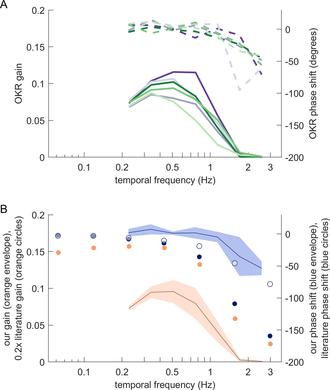
Magnitude and phase shift of eye movements at different frequencies resemble those previously observed for zebrafish OKR.
(A) Bode plots showing OKR gain (solid lines) and phase shift relative to the stimulus (dashed lines). Gains and phase shifts decrease as temporal frequency increases. Each line represents the mean across trials for a specific stimulus location, pooled across all fish, all trials and both eyes. Colours match the stimulus locations identified in Figure 5c. (B) Our observations qualitatively, but not quantitatively, match those reported for traditional full-field stimulus paradigms. Solid blue circles represent OKR phase shifts for approximately 6.4 dpf zebrafish larvae reported by Beck et al., 2004. The blue line represents our own mean phase shift across all stimulus locations shown in (A), and the light blue envelope shows the standard deviation across locations. Interestingly, our phase shifts are more in line with those reported for older fish (approximately 33.8dpf larvae, open blue circles) in Beck et al., 2004. Solid orange circles show scaled OKR gain for approximately 6.4dpf zebrafish larvae, as reported by Beck et al., 2004. Direct comparison to our gain data could be misleading because of the smaller size and higher velocity of our stimuli. Based on our results reported in Figure 5e, the size difference alone should account for a factor of about 5. Orange circles thus show the literature gain data scaled 0.2x. The black line and orange envelope represent our mean OKR gain and standard deviation across all stimulus locations shown in (A). Quantitative changes are consistent with the notion that smaller and faster stimuli evoke equally reliable, but lower-amplitude OKR behaviour (Figure 2c).
Figure 5—figure supplement 2
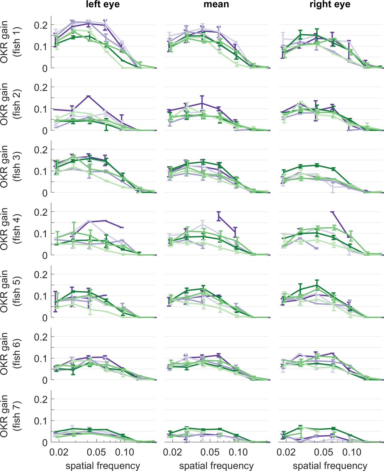
OKR gain of individual larvae, for different stimulus frequencies.
Same colours as in Figure 5. Error bars show standard error of the mean. Data from n = 7 fish.
Figure 5—figure supplement 3

OKR gain of individual larvae, for different stimulus sizes.
Same colours as in Figure 5. Error bars show standard error of the mean. Data from n = 7 fish.
Figure 5—video 1
Animation showcasing short samples of all disk stimuli used to study frequency dependence, as in Figure 5a.
Figure 5—video 2
Animation showcasing short samples of all disk stimuli used to study size dependence, as in Figure 5b.
Figure 6 with 1 supplement
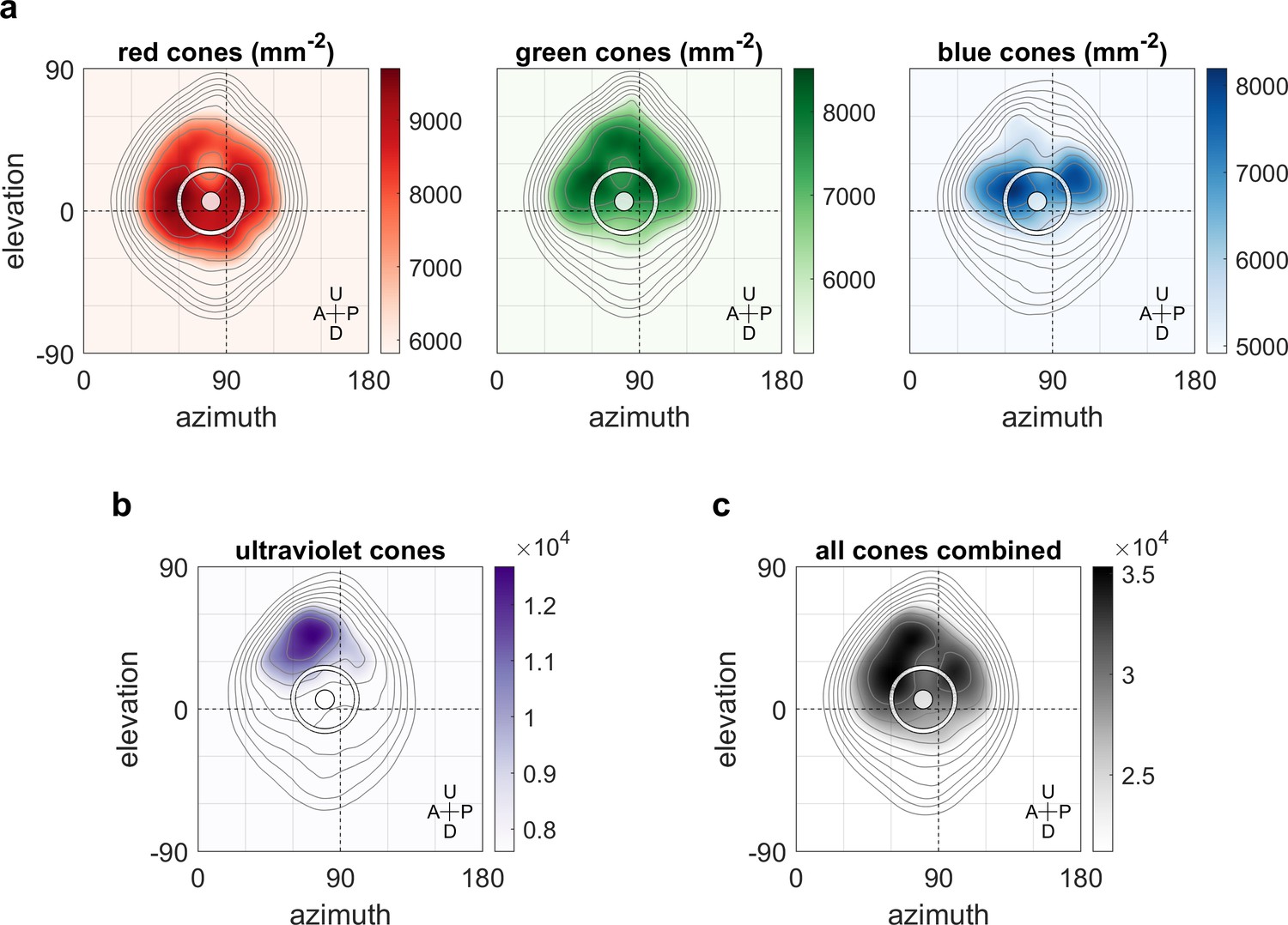
Maximum OKR gain is consistent with high photoreceptor densities in the retina.
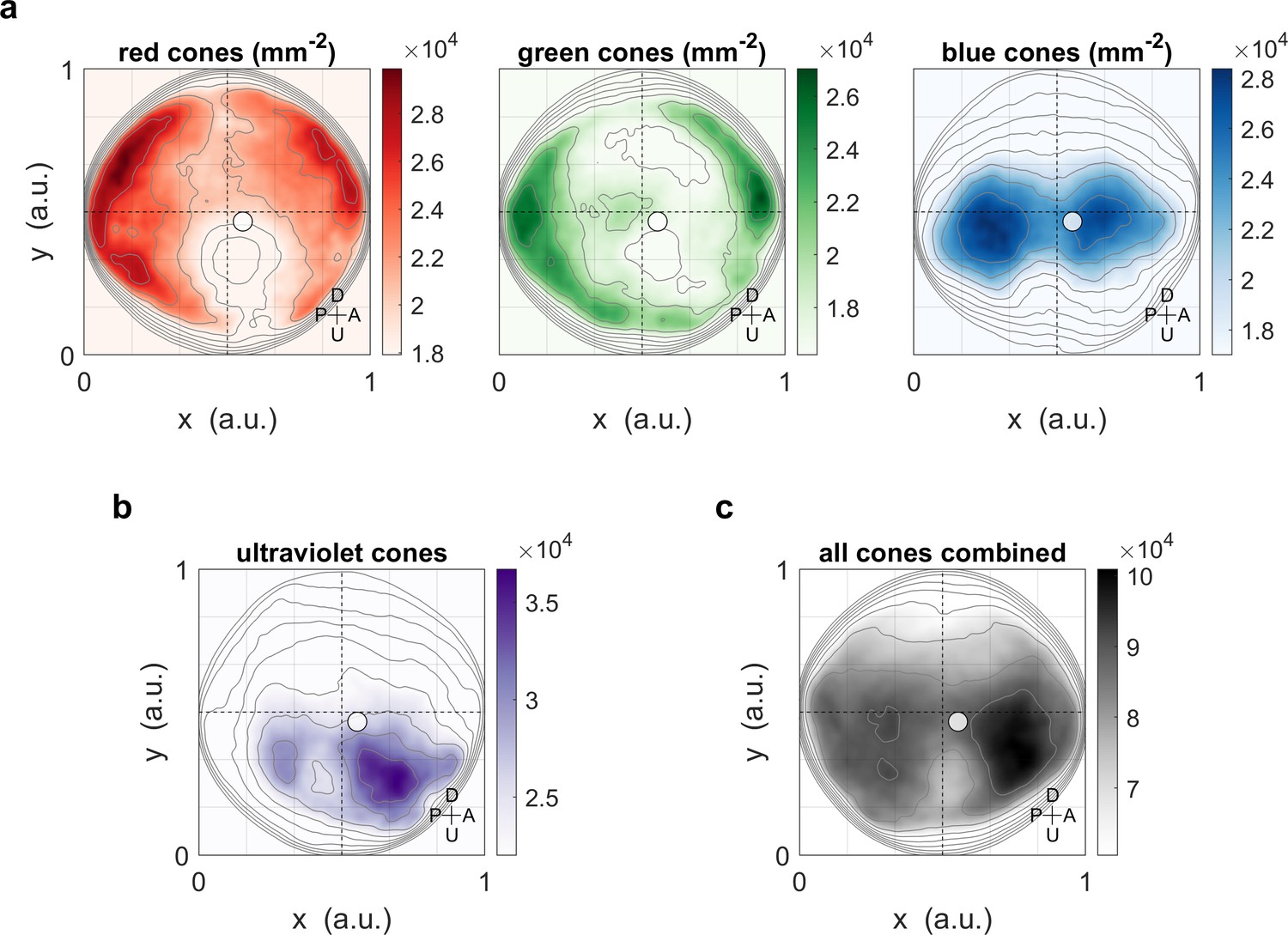
Contour lines show retinal photoreceptor density determined by optical measurements of explanted eye cups of 7–8 dpf zebrafish larvae, at increments of 10% of maximum density. Data shown in visual space coordinates relative to the body axis, that is, 90° azimuth and 0° elevation corresponds to a perfectly lateral direction. To highlight densely covered regions, densities from half-maximum to maximum are additionally shown in shades of colour. Solid white circles indicate the location of maximum OKR gain inferred from experiments of type D in 5-7dpf larvae (Figure 3). White outlines indicate the area that would be covered by a 40° disk-shaped stimulus centred on this location when the eye is in its resting position. As the eyes move within their beating field during OKR, the actual, non-stationary retinal coverage extends further rostrally and caudally. For (a) red, green, and blue photoreceptors, high densities coincide with high OKR gains. (b) For ultraviolet receptors, there is no clear relationship to the OKR gain. (c) For reference, the summed total density of all receptor types combined. We did not observe a significant shift in the position-dependence of maximum OKR gain between groups of larvae at 5, 6, or 7 dpf of age, consistent with the notion that retinal development is far advanced and the circuits governing OKR behaviour are stable at this developmental stage. U: Up, D: Down, A: Anterior, P: Posterior.
-
Figure 6—source data 1
Numerical data and graphical elements of Figure 6.
- https://cdn.elifesciences.org/articles/63355/elife-63355-fig6-data1-v2.mat
Figure 6—figure supplement 1
Maximum OKR gain compared to photoreceptor densities in retinal coordinates.
Same as Figure 6, but showing positions across the retina in Cartesian coordinates, as originally published (Zimmermann et al., 2018 Curr Biol), instead of in geographic visual field coordinates. When plotting photoreceptor densities in Cartesian coordinates, the regions of highest densities appear to be located quite peripheral/eccentric. However, the plot of the densities in visual field coordinates (Figure 6) confirms the coincidence of high densities and high OKR gains. Solid circles indicate the location of maximum OKR gain inferred from experiments of type D in 5-7 dpf larvae (Figure 3), and corrected by the mean eye position over time. U: Up, D: Down, A: Anterior, P: Posterior.
Videos
Video 1
Repulsion-based algorithm to numerically distribute stimulus centres across a sphere surface (Source code 1B), with gradual convergence on a logarithmic timescale (blue to green).
A subset of stimulus centres is held on the equator at zero elevation (orange).
Tables
Key resources table
| Reagent type (species) or resource | Designation | Source or reference | Identifiers | Additional information |
|---|---|---|---|---|
| Genetic reagent (Danio rerio) | mitfas184 | https://zfin.org/action/genotype/view/ZDB-GENO-080305-2, (Scott et al., 2007) | RRID:ZFIN_ZDB-ALT-070629-2 | Mutant fish line (melanocyte inducing transcription factor a) |
| Software, algorithm | ZebEyeTrack | http://zebeyetrack.org/, (Dehmelt et al., 2018) | DOI:10.1038/s41596-018-0002-0 | Modular eye tracking software for zebrafish |
| Software, algorithm | spherical arena code | https://gin.g-node.org/Arrenberg_Lab/spherical_arena, (Dehmelt et al., 2020) | DOI:10.12751/g-node.qergnn | Code for stimulus generation, LED position mapping, and arena control |
| Software, algorithm | OpenSCAD | https://www.openscad.org/ | 3D computer-aided design of arena scaffold | |
| Other | LED array | Kingbright Electronic Co. | TA08-81CGKWA | Green light emitting LED tiles, 20 × 20 mm each, peak power at 568 nm |
| Other | hardware controller | Joesch et al., 2008 | DOI:10.1016/j.cub.2008.02.022 | Circuit board designs and code by Alexander Borst (MPI Neurobiol, Martinsried), Väinö Haikala and Dierk Reiff (University of Freiburg) |
Author response table 1
| regular arena | azimuth 1 | elevation 1 | azimuth 2 | elevation 2 |
|---|---|---|---|---|
| fish no. 1 | -77.6 | 7.5 | 70.7 | 9.2 |
| fish no. 2 | -78.7 | 6.4 | 52.9 | 13.2 |
| fish no. 3 | -76.5 | 8.2 | 64.7 | 8.0 |
| fish no. 4 | -78.7 | 6.4 | 52.9 | 13.2 |
| fish no. 5 | -77.9 | 5.3 | 92.6 | 0.0 |
| fish no. 6 | -90.7 | 3.3 | 84.8 | -2.9 |
| fish no. 7 | -83.2 | 9.9 | 91.9 | -3.3 |
Author response table 2
| rotated arena | azimuth 1 | elevation 1 | azimuth 2 | elevation 2 |
|---|---|---|---|---|
| fish no. 1* | -27.4 | 34.2 | 141.5 | -39.6 |
| fish no. 2 | -64.9 | 10.3 | 71.7 | -9.6 |
| fish no. 3 | -76.3 | 0.9 | 86.7 | 4.5 |
| fish no. 4 | -97.9 | 7.6 | 73.1 | -6.6 |
| fish no. 5 | -93.3 | -1.9 | 76.9 | 4.8 |
Additional files
-
Source code 1
Five separate sets of MATLAB code.
(A) Code to design visual stimuli, convert them to geographic coordinates, and map them onto the actual position of individual LEDs. (B) Code to numerically identify a distribution of nearly equidistant stimulus centres that is symmetric between the left and right, upper and lower, as well as front and rear hemispheres. (C) Code to read raw eye traces, identify individual stimulus phases, detect and remove saccades, compute piece-wise fits to cropped and pre-processed raw data, and return OKR gains. (D) Code to recreate the results figures from data, especially Figure 3, Figure 5, Figure 6. (E) Code to assess the significance of differences between the best fits to data for fish embedded upright or upside-down. This last set of code requires access to the raw data repository.
- https://cdn.elifesciences.org/articles/63355/elife-63355-code1-v2.zip
-
Supplementary file 1
Seven supplementary tables.
(A) The arena cross-section, (B) stimulus parameters for position dependence experiments, (C) absolute positions of fish and setup elements in different experiments, (D) stimulus parameters for control experiments, (E) parameters for whole-field and hemisphere stimuli, (F) stimulus parameters for frequency dependence experiments, and (G) stimulus parameters for size dependence experiments.
- https://cdn.elifesciences.org/articles/63355/elife-63355-supp1-v2.docx
-
Transparent reporting form
- https://cdn.elifesciences.org/articles/63355/elife-63355-transrepform-v2.docx
Download links
A two-part list of links to download the article, or parts of the article, in various formats.
Downloads (link to download the article as PDF)
Open citations (links to open the citations from this article in various online reference manager services)
Cite this article (links to download the citations from this article in formats compatible with various reference manager tools)
Spherical arena reveals optokinetic response tuning to stimulus location, size, and frequency across entire visual field of larval zebrafish
eLife 10:e63355.
https://doi.org/10.7554/eLife.63355


