Bi-channel image registration and deep-learning segmentation (BIRDS) for efficient, versatile 3D mapping of mouse brain
- School of Optical and Electronic Information- Wuhan National Laboratory for Optoelectronics, Huazhong University of Science and Technology, China
- School of Basic Medicine, Tongji Medical College, Huazhong University of Science and Technology, China
- Britton Chance Center for Biomedical Photonics, Wuhan National Laboratory for Optoelectronics, Huazhong University of Science and Technology, China
Figures
Figure 1 with 4 supplements
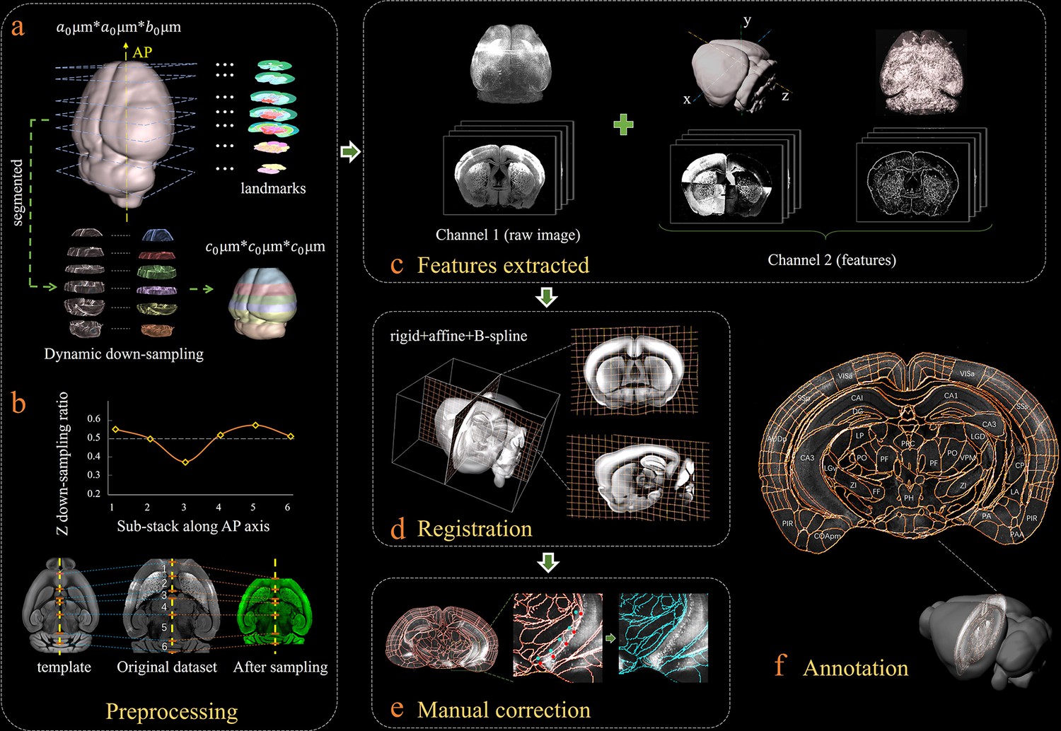
Bi-channel brain registration procedure.
(a) Re-sampling of a raw 3D image into an isotropic low-resolution one, which has the same voxel size (20 μm) using an averaged Allen template image. The raw brain dataset was first subdivided into six sub-stacks along the AP axis according to landmarks identified in seven selected coronal planes (a1). Then an appropriate z re-sampling ratio, which was different for each slice, was applied to each sub-stack (a2, left) to finely adjust the depth of the stack in the down-sampled data (a2, right). This step roughly restored the deformation of non-uniformly morphed samples, thereby allowing the following registration with an Allen reference template. (b) Plot showing the variation of the down-sampling ratio applied to the six sub-stacks and comparison with the Allen template brain before and after the dynamic re-sampling showing the shape restoration effects of the this preprocessing step. (c) Additional feature channels containing a geometry and outline feature map extracted using grayscale reversal processing (left), as well as an edge and texture feature map extracted by a phase congruency algorithm (right). This feature channel was combined with a raw image channel for implementing our information-enriched bi-channel registration, which showed improved accuracy as compared to conventional single-channel registration solely based on raw images. (d) 3D view and anatomical sections (coronal and sagittal planes) of the registration results displayed in a grid deformed from an average Allen template. (e) Visual inspection and manual correction of automatically-registered results from an optically clarified brain, which showed obvious deformation. Using the GUI provided, this step could be readily operated by adjusting the interactive nodes in the annotation file (red points to light blue points). (f) A final atlas of an experimental brain image containing region segmentations and annotations.
Figure 1—figure supplement 1
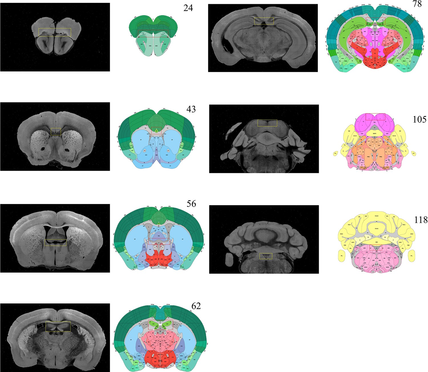
Selection of featured coronal planes corresponded to the Allen Reference Atlas, for subdividing the entire brain volume into multiple sub-stacks along AP axis.
The GUI of BIRDS program first permits the selection of a series of coronal planes (monochrome images) from the deformed 3D brain data, which are corresponded to the Allen Reference Atlas (#23, 43, 56, 62, 78, 105, and 118 of total 132 slices). The selection of coronal planes corresponded to the Allen Reference Atlas is based on the identification of several anatomical features, as shown in the paired yellow-red rectangular boxes. Then the six sub-stacks segmented according to these seven planes are processed with different down-sampling ratios (from 0.36 to 0.59, Figure 1b), to obtain the corresponding rectified stacks with 1:1 scale ratio to the Allen template images (total 660 slice, 20 μm resolution). These rectified sub-stacks are finally combined to form an entire 3D brain volume with restored shape more similar to the Allen average template.
Figure 1—figure supplement 2
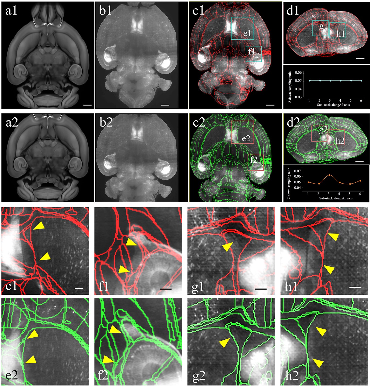
Improved registration accuracy enabled by the abovementioned shape rectification preprocessing.
(a–d) Automatical registration results of the experimental brain data obtained after applying conventional uniform (top panel, a1–d1) and our non-uniform down-sampling (bottom panel, a2–d2), respectively. From (a) to (d), we comparatively show the moving template image (a1, a2), fixed experimental image (b1, b2), and corresponding segmentation results in horizontal (c1, c2) and coronal views (d1, d2), respectively. Scale bars, 1 mm. (e, f) Magnified views of two region-of-interests (boxes) shown in the registered-and-annotated horizontal planes (c1, c2). The yellow arrows indicate the improved accuracy by our BIRDS method (e2, f2), as compared to conventional uniform down-sampling registration (e1, f1). (g, h) Magnified views of two region-of-interests (boxes) in registered-and-annotated coronal planes (d1, d2). The yellow arrows indicate the improved accuracy by our method (g2, h2), as compared to conventional uniform down-sampling registration (g1, h1). Scale bar, 250 μm.
Figure 1—figure supplement 3
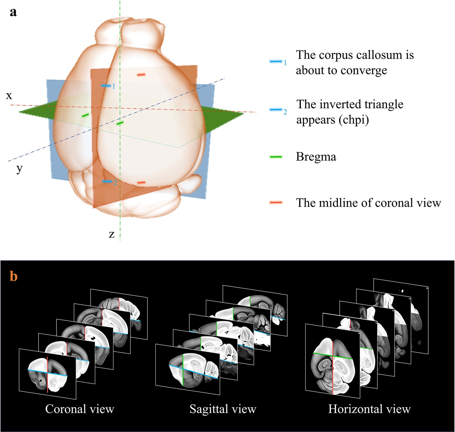
Extraction of axes features for registration.
(a) Determination of sagittal (orthogonal to lateral-medial axis, orange); horizontal (orthogonal to dorsal-ventral axis, blue); and coronal (orthogonal to anterior–posterior axis, green) planes based on the identification of specific anotomical features, as shown in (a). (b) Grayscale reversal processing applied to the background-filtrated image dataset, according to the above-defined axis planes. The extraction of pure signals together with artificial reversal operation generate an extra feature map containing the geometry information of the axes, which is benefical to the improvement of registration accuracy.
Figure 1—figure supplement 4
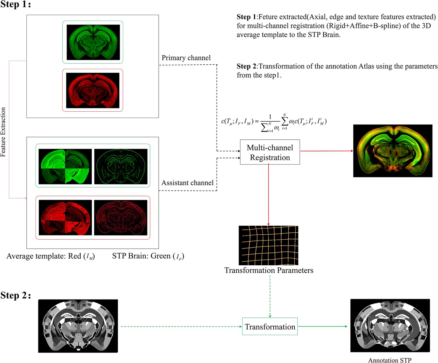
Schematic of the multi-channel registration and annotation process.
For both experimental and template data, an additional feature channel (assistant channel) containing texture features extracted by PC and axial geometry features added by grayscale reversal, are combined with the raw image channel (primary channel) to implement information-augmented dual-channel registration based on rigid, affine, and B-spline transformation. This procedure simultaneously registers all the multi-spectral input data using a single cost function, as shown in Step 1. The transformation parameters obtained from the image registration procedure are then applied to the template mouse annotation atlas (Allen Institute, CCF v3) to transform the template annotation file into an individual one that specifically fits our experimental brain image, and thus describes the anatomical structures in the whole-brain space (Step 2).
Figure 2 with 4 supplements
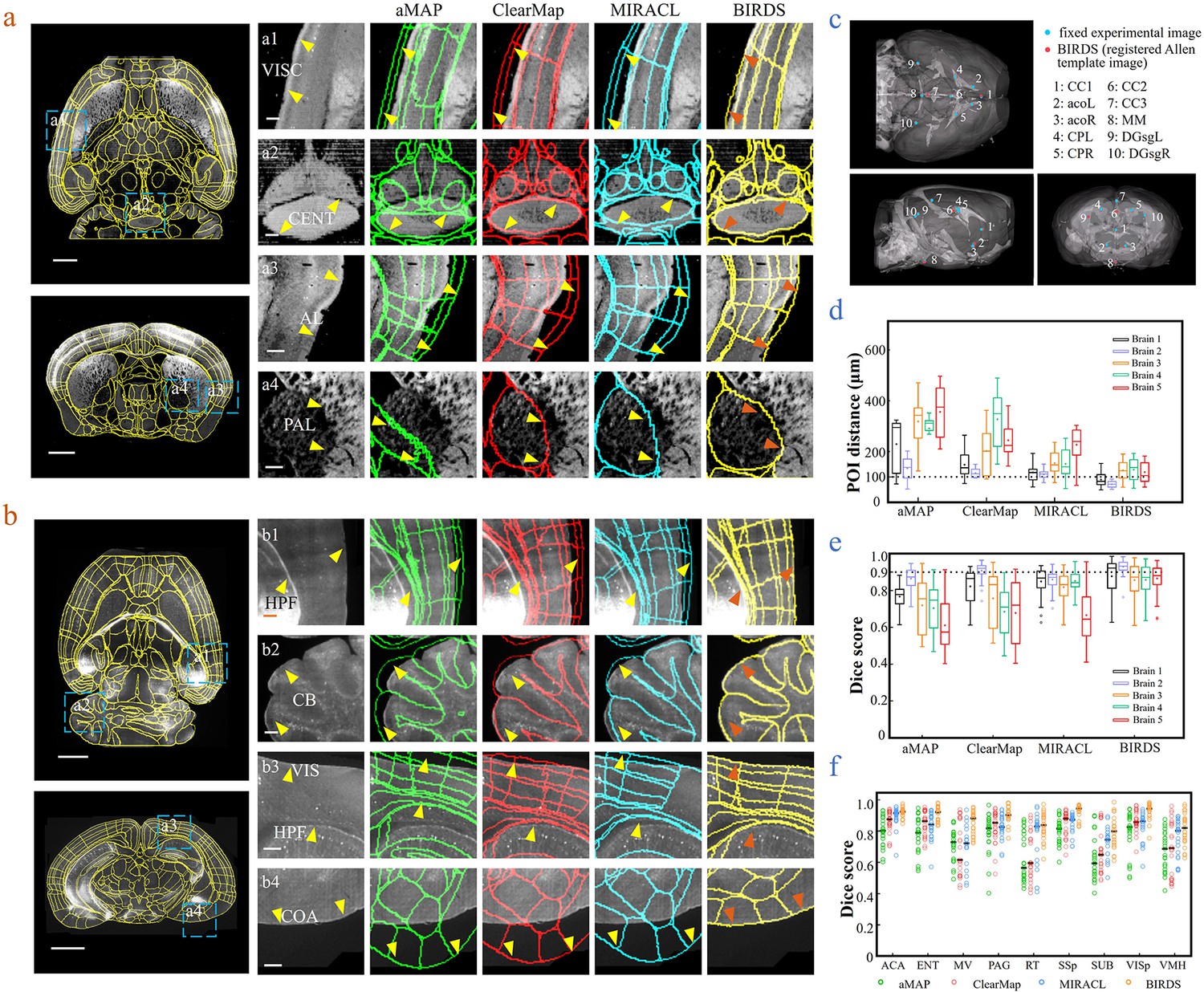
Comparison of BIRDS with conventional single-channel registration methods.
(a) Comparative registration accuracy (STPT data from an intact brain) using four different registration methods, aMAP, ClearMap, MIRACL, and BIRDS. (b) Comparative registration accuracy (LSFM data from clarified brain) using four methods. Magnified views of four regions of interest (a1–a4, b1–b4, blue boxes) selected from the horizontal (left, top) and coronal planes (left, bottom) are shown in the right four columns, with 3D detail for the registration/annotation accuracy for each method. All comparative annotation results were directly output from respective programs without manual correction. Scale bar, 1 mm (whole-brain view) and 250 μm (magnified view). (c) Ten groups of 3D fiducial points of interest (POIs) manually identified across the 3D space of whole brains. The blue and red points belong to the fixed experimental images and the registered Allen template images, respectively. The ten POIs were selected from the following landmarks: POIs: cc1: corpus callosum, midline; acoL, acoR: anterior commisure, olfactory limb; CPL, CPR: Caudoputamen, Striatum dorsal region; cc2: corpus callosum, midline; cc3: corpus callosum, midline; MM: medial mammillary nucleus, midline; DGsgL, DGsgR: dentate gyrus, granule cell layer. The registration error by each method could be thereby quantified through measuring the Euclidean distance between each pair of POIs in the experimental image and template image. (d) Box diagram comparing the POI distances of five brains registered by the four methods. Brains 1, 2: STPT images from two intact brains. Brain one is also shown in (a). Brains 3, 4, and 5: LSFM images from three clarified brains (u-DISCO) that showed significant deformations. Brain five is also shown in (b). The median error distance of 50 pairs of POIs in the five brains registered by BIRDS was ~104 μm, as compared to ~292 μm for aMAP, ~204 μm for ClearMap, and ~151 μm for MIRACL. (e, f) Comparative plot of Dice scores in nine registered regions of the five brains. The results were grouped by brain in (e) and region in (f). The calculation was implemented at the single nuclei level. When the results were analyzed by brain, BIRDS surpassed the other three methods most clearly using LSFM dataset #5, with a 0.881 median Dice score as compared to 0.574 from aMAP, 0.72 from ClearMap, and 0.645 from MIRACL. At the same time, all the methods performed well on STPT dataset #2, with a median Dice score of 0.874 from aMAP, 0.92 from ClearMap, 0.872 from MIRACL, and 0.933 from BIRDS. When the results were compared using nine functional regions, the median values acquired by BIRDS were also higher than the other three methods. Even the lowest median Dice score by our method was still 0.799 (indicated by black line), which was notably higher than 0.566 by aMAP, 0.596 by ClearMap, and 0.722 by MIRACL, respectively.
-
Figure 2—source data 1
Source data file for Figure 2.
- https://cdn.elifesciences.org/articles/63455/elife-63455-fig2-data1-v3.zip
Figure 2—figure supplement 1
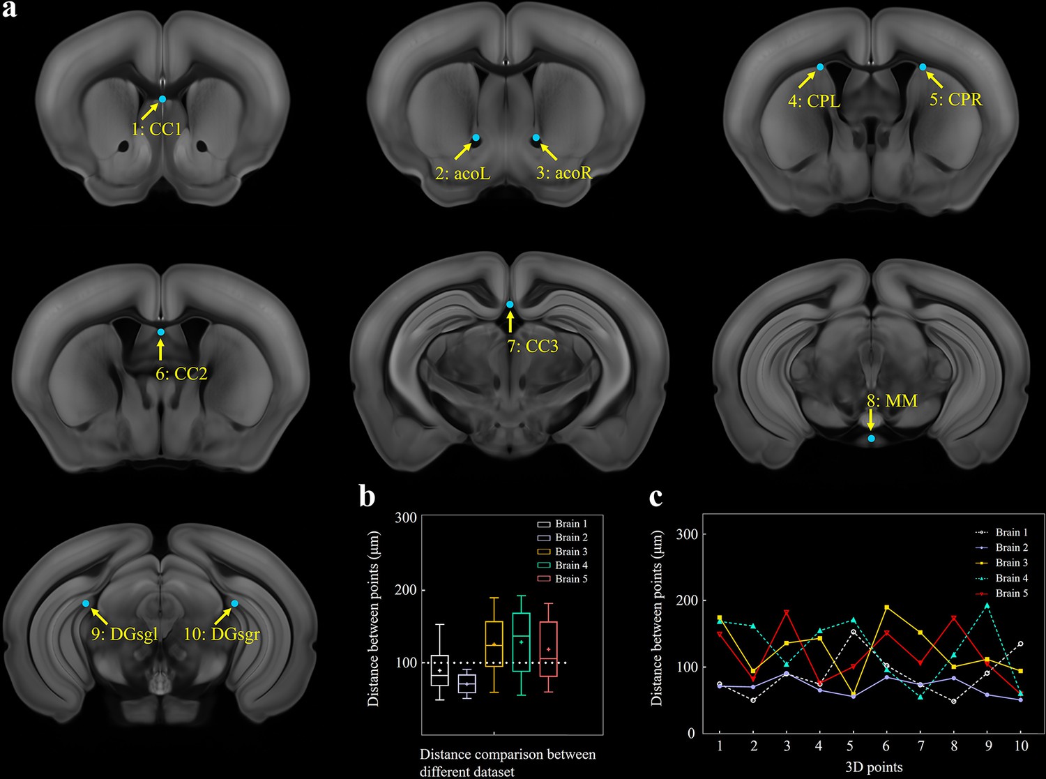
Selection of 10 fiducial points of interest (POIs) for measuring the error distance between registered brains.
(a) Ten selected feature points in Allen template image. (1) cc1: corpus callosum, midline. (2, 3) acoL, acoR: anterior commisure, olfactory limb. (4, 5) CPL, CPR: Caudoputamen, Striatum dorsal region. (6) cc2: corpus callosum, midline. (7) cc3: corpus callosum, midline. (8) MM: medial mammillary nucleus, midline. (9, 10) DGsgL, DGsgR: dentate gyrus, granule cell layer. (b) Box diagrams showing the error distances between the paired POIs in registered template and experimental brains (n = 5 brains, which are also used for Figure 2). Using BIRDS method, the median error distance of total 50 pairs of POIs in five brains is ~104 μm. (c) Line plot further showing the distance between each pair of POI.
Figure 2—figure supplement 2
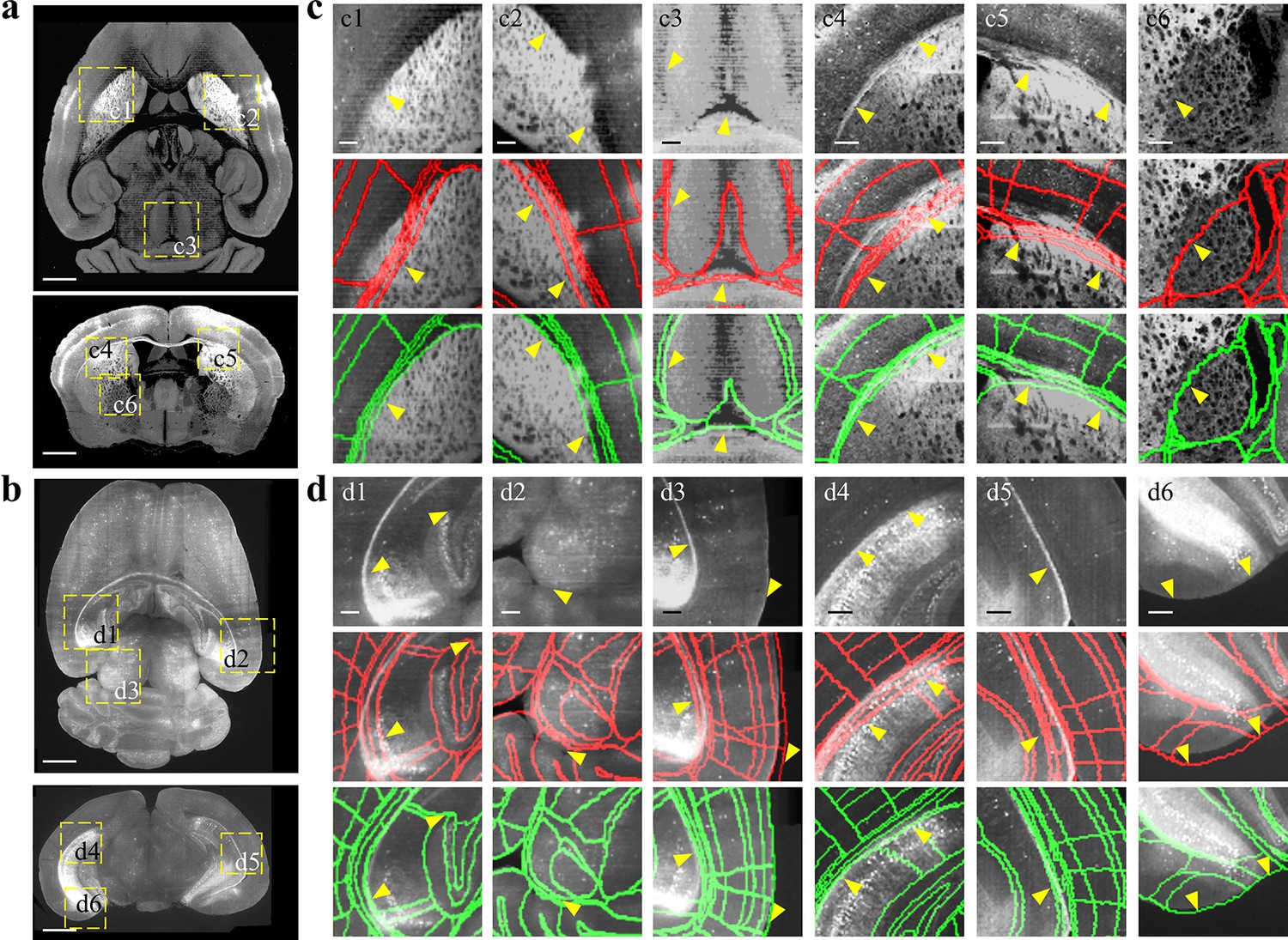
Comparison between BIRDS and conventional single-channel registration.
(a, b) STPT image of intact brain and LSFM image of clarified brain, which are registered by our BIRDS and conventional single-channel method. (c, d) Magnified views of six region-of-interests (yellow boxes) selected from the horizontal (top in a, b) and coronal planes (bottom in a, b) in the STPT and LSFM brains, respectively. The comparison between BIRDS (green annotation) and single-channel (red annotation) results indicates obviously less inaccuracy by our BIRDS method (yellow arrows). All segmentation results are directly outputted from the programs, without any manual correction. Scale bar, 1 mm for (a, b) and 250 μm for (c, d).
Figure 2—figure supplement 3
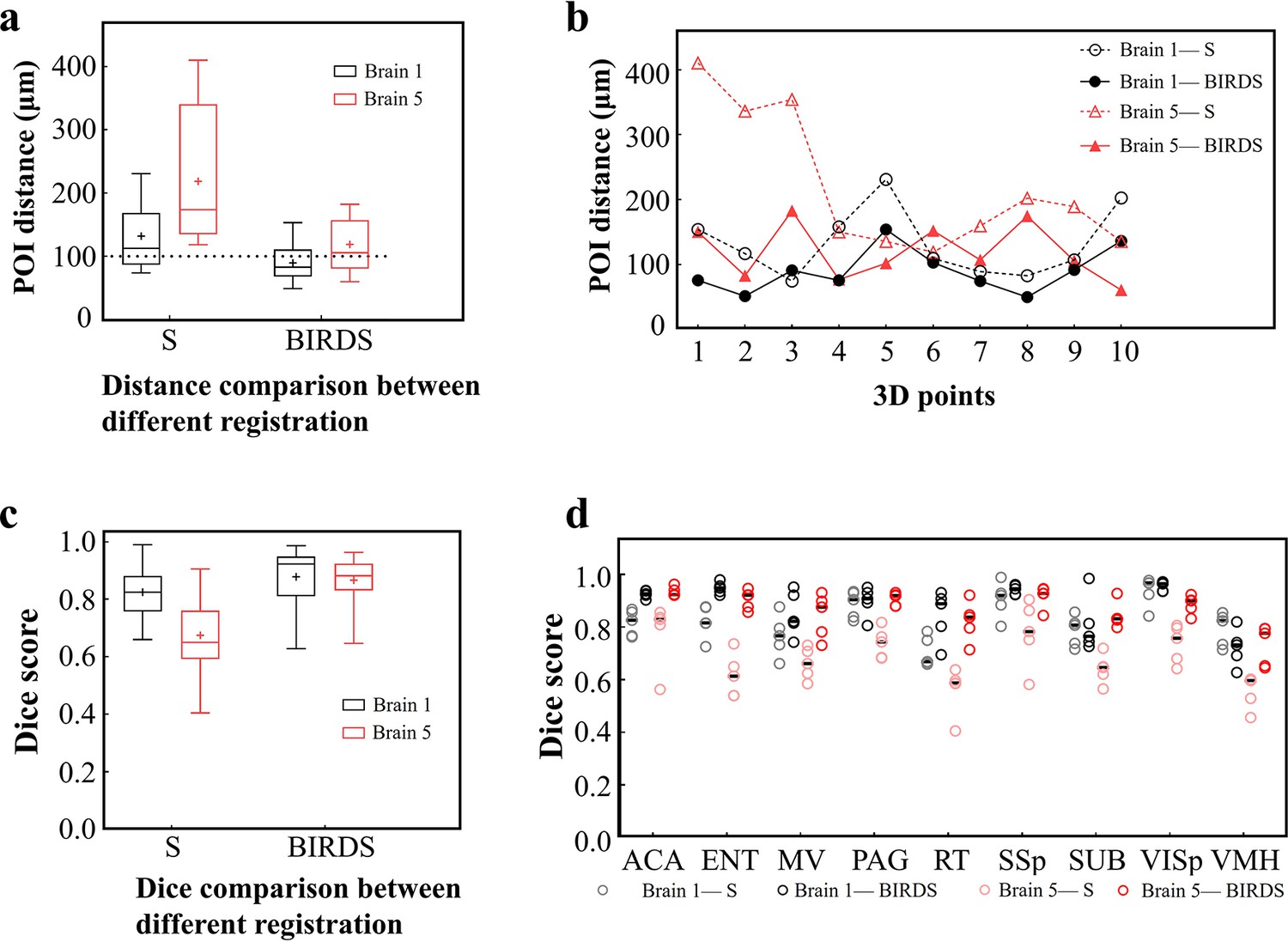
Comparative accuracy analysis of BIRDS and single-channel registration.
(a) Box diagram showing the distances between the paired POIs (Figure 2—figure supplement 1) in Allen template and experimental image registered by BIRDS and conventional single-channel registration. Black Brain 1 represents STPT image of an intact brain, and red Brain 5 represents LSFM image of a clarified brain, which have been also shown in Figure 2—figure supplement 2. The median error distance of 20 pairs of POIs in the two brains registered by BIRDS is ~104 μm, which is compared to ~175 μm error distance by single-channel registration. (b) Line chart specifically showing the distance of each pair of points in two types of datasets by two registration methods. Besides smaller median error distance, here BIRDS registration with including feature information also yields smaller distance variance (solid lines), as compared to single-channel method (dash line). (c) Dice score comparison of two registration methods at nuclei level. Eighteen regions in two brains (nine regions for each) are selected for the analysis, with results grouped by the datasets. It is clearly shown that the median Dice scores by our method are higher than those by single-channel registration, especially for the highly deformed clarified brain (Brain 5, 0.65 vs 0.881). (d) Dice scores of two registration methods, with results grouped by nine selected sub-regions (five planes included for each region), which are ACA, ENT, MV, PAG, RT, SSp, SUB, VISp, and VMH. The black lines indicate the median Dice scores for each regions. Overall, Dice scores with averaged median value of >0.9 (calculated by two brains) or >0.87 (calculated by nine regions) were obtained by our BIRDS. These two values are obviously higher than 0.74 and 0.76 by single-channel registration.
-
Figure 2—figure supplement 3—source data 1
Source data file for Figure 2—figure supplement 3.
- https://cdn.elifesciences.org/articles/63455/elife-63455-fig2-figsupp3-data1-v3.zip
Figure 2—figure supplement 4
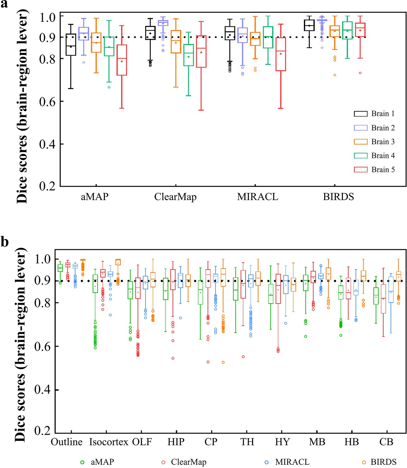
Dice score comparison of nine regions in five brains registered by four registration tools: aMAP, ClearMap, MIRACL, and our BIRDS.
The results are grouped by brains in (a) and regions in (b). The calculation/comparison is implemented at region level with ~100 μm resolution. When the results are analyzed by brains, BIRDS surpass the other three methods most on LSFM dataset #5, with 0.944 median Dice score being compared to 0.801 by aMAP, 0.848 by ClearMap, and 0.835 by MIRACL. At the same time, all the methods perform well on STPT dataset #2 with median Dice of 0.919 by aMAP, 0.969 by ClearMap, 0.915 by MIRACL, and 0.977 by our BIRDS. When the results are compared by nine functional regions, the median values acquired by our BIRDS were also higher than the other three methods. Even the lowest median Dice score by our method is still 0.885 (indicated by black line), which is notably higher than 0.834 by aMAP, 0.82 by ClearMap, and 0.853 by MIRACL.
-
Figure 2—figure supplement 4—source data 1
Source data file for Figure 2—figure supplement 4.
- https://cdn.elifesciences.org/articles/63455/elife-63455-fig2-figsupp4-data1-v3.zip
Figure 3
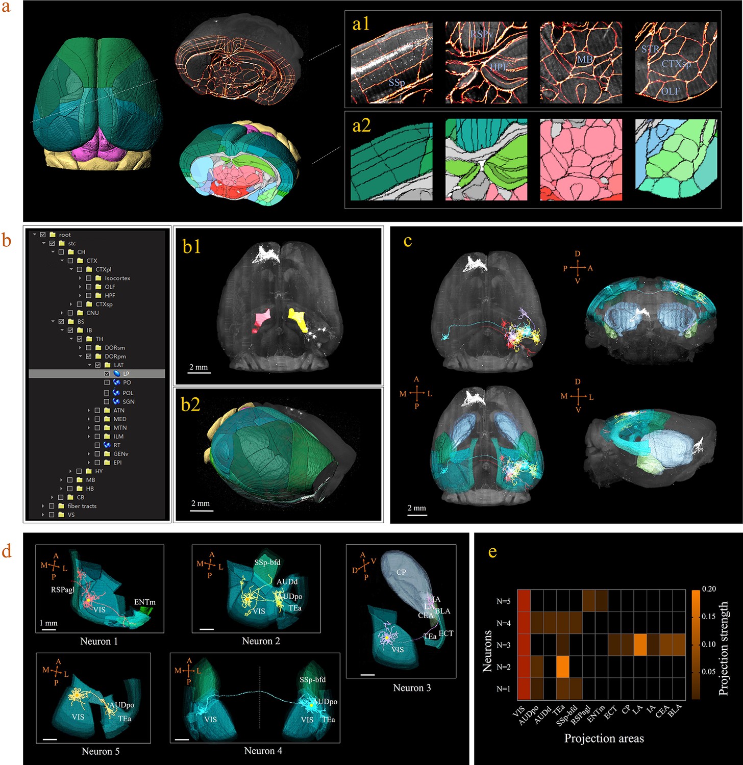
3D digital atlas of a whole brain for visualization and quantitative analysis of inter-areal neuronal projections.
(a) Rendered 3D digital atlas of a whole brain (a2, pseudo color), which was generated from registered template and annotation files (a1, overlay of annotation mask and image data). (b) Interactive hierarchical tree shown as a sidebar menu in the BIRDS program, indexing the name of brain regions annotated in CCFv3. Clicking on any annotation name in the side bar of the hierarchal tree highlights the corresponding structure in the 3D brain map (b1, b2), and vice versa. For example, brain region LP was highlighted in the space after its name was chosen in the menu (b1). 3D rendering of an individual brain after applying a deformation field in reverse to a whole brain surface mask. The left side of the brain displays the 3D digital atlas (CCFv3, colored part in b2), while the right side of the brain is displayed in its original form (grayscale part in b2). (c) The distribution of axonal projections from five single neurons in 3D map space. The color-rendered space shown in horizontal, sagittal, and coronal views highlights multiple areas in the telencephalon, anterior cingulate cortex, striatum, and amygdala, which are all potential target areas of layer-2/3 neuron projections. (d) The traced axons of five selected neurons (n = 5) are shown. ENTm, entorhinal area, medial part, dorsal zone; RSPagl, retrosplenial area, lateral agranular part; VIS, visual areas; SSp-bfd, primary somatosensory area, barrel field; AUDd, dorsal auditory area; AUDpo, posterior auditory area; TEa, temporal association areas; CP, caudoputamen; IA, intercalated amygdalar nucleus; LA, lateral amygdalar nucleus; BLA, basolateral amygdalar nucleus; CEA, central amygdalar nucleus; ECT, ectorhinal area. (e) Quantification of the projection strength across the targeting areas of five GFP-labeled neurons. The color codes reflect the projection strengths of each neuron, as defined as axon length per target area, normalized to the axon length in VIS.
-
Figure 3—source data 1
Source data file for Figure 3e.
- https://cdn.elifesciences.org/articles/63455/elife-63455-fig3-data1-v3.zip
Figure 4
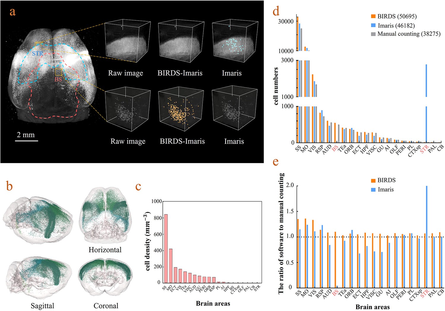
Cell-type-specific counting and comparison between different cell counting methods.
(a) Cell counting of retrogradely labeled striatum-projecting cells. We selected two volumes (1 × 1 × 1 mm3) from SS and VIS areas, respectively, to show the difference in cell density and the quantitative results by BIRDS–Imaris versus conventional Imaris. Here, a separate quantification parameters set for different brain areas in the BIRD–Imaris procedure lead to obviously more accurate counting results. Scale bar, 2 mm. (b) 3D-rendered images of labeled cells in the whole brain space, shown in horizontal, sagittal, and coronal views. The color rendering of the cell bodies was in accordance with CCFv3, and the cells were mainly distributed in the Isocortex (darker hue). (c) The cell density calculated for 20 brain areas. The cell densities of MO and SS were highest (MO = 421.80 mm−3; SS = 844.71 mm−3) among all areas. GU, gustatory areas; TEa, temporal association areas; AI, agranular insular area; PL, prelimbic area; PERI, perirhinal area; RSP, retrosplenial area; ECT, ectorhinal area; ORB, orbital area; VISC, visceral area; VIS, visual areas; MO, somatomotor areas; SS, somatosensory areas; AUD, auditory areas; HPF, hippocampal formation; OLF, olfactory areas; CTXsp, cortical subplate; STR, striatum; PAL, pallidum; BS, brainstem; CB, cerebellum. (d) Comparison of the cell numbers from three different counting methods, BIRDS, Imaris (3D whole brain directly), and manual counting (2D slice by slice for a whole brain). (e) The cell counting accuracy using BIRDS–Imaris (orange) and conventional Imaris methods (blue), relative to manual counting. Besides the highly divergent accuracy for the 20 regions, the counting results by conventional Imaris in STR and BS regions were especially inaccurate.
-
Figure 4—source data 1
Source data file for Figure 4.
- https://cdn.elifesciences.org/articles/63455/elife-63455-fig4-data1-v3.zip
Figure 5 with 5 supplements
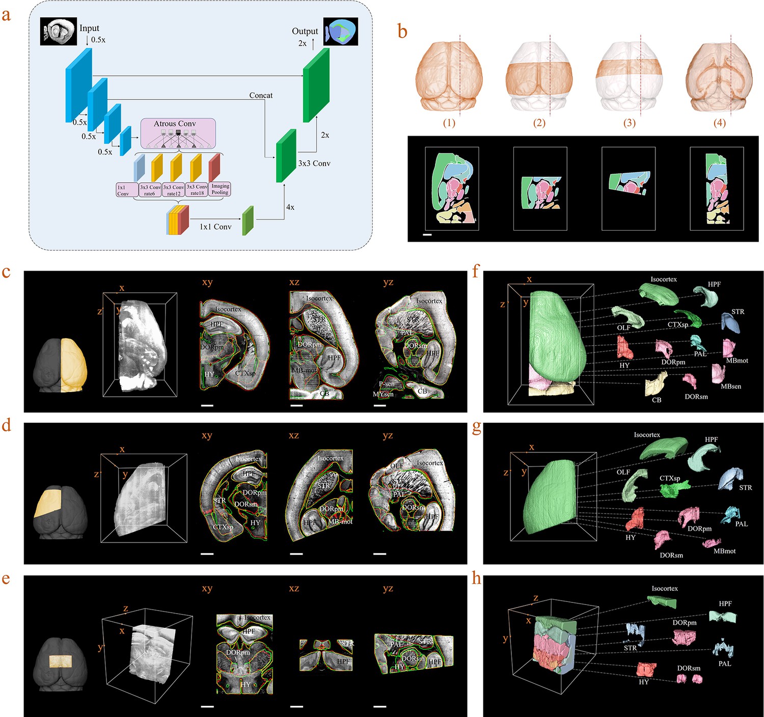
Inference-based network segmentation of incomplete brain data.
(a) The deep neural network architecture for directly inferring brain segmentation without required registration. The training datasets contained various types of incomplete brain images, which were cropped from annotated whole-brain datasets created using our bi-channel registration beforehand. (b) Four models of incomplete brain datasets for network training: whole brain (1), a large portion of telencephalon (2), a small portion of telencephalon (3), and a horizontal slab of whole brain (4). Scale bar, 1 mm. (c–e) The inference-based segmentation results for three new modes of incomplete brain images, defined as the right hemisphere (c), an irregular cut of half the telencephalon (d), and a randomly cropped volume (e). The annotated sub-regions are shown in the x-y, x-z, and y-z planes, with the Isocortex, HPF, OLF, CTXsp, STR, PAL, CB, DORpm, DORsm, HY, MBsen, MBmot, MBsta, P-sen, P-mot, P-sat, MY-sen, and MY-mot for right hemisphere, Isocortex, HPF, OLF, CTXsp, STR, PAL, DORpm, DORsm, HY, and MY-mot for the irregular cut of half the telencephalon, and Isocortex, HPF, STR, PAL, DORpm, DORsm, and HY for the random volume. Scale bar, 1 mm. (f–h) Corresponding 3D atlases generated for these three incomplete brains.
-
Figure 5—source data 1
Source data file for Figure 5.
- https://cdn.elifesciences.org/articles/63455/elife-63455-fig5-data1-v3.zip
Figure 5—figure supplement 1
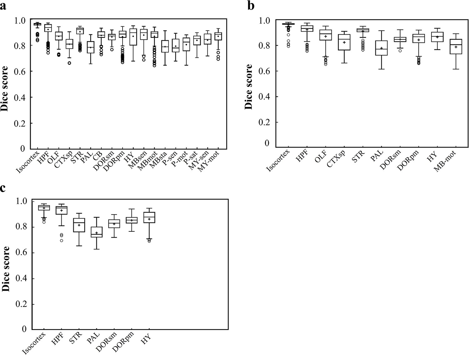
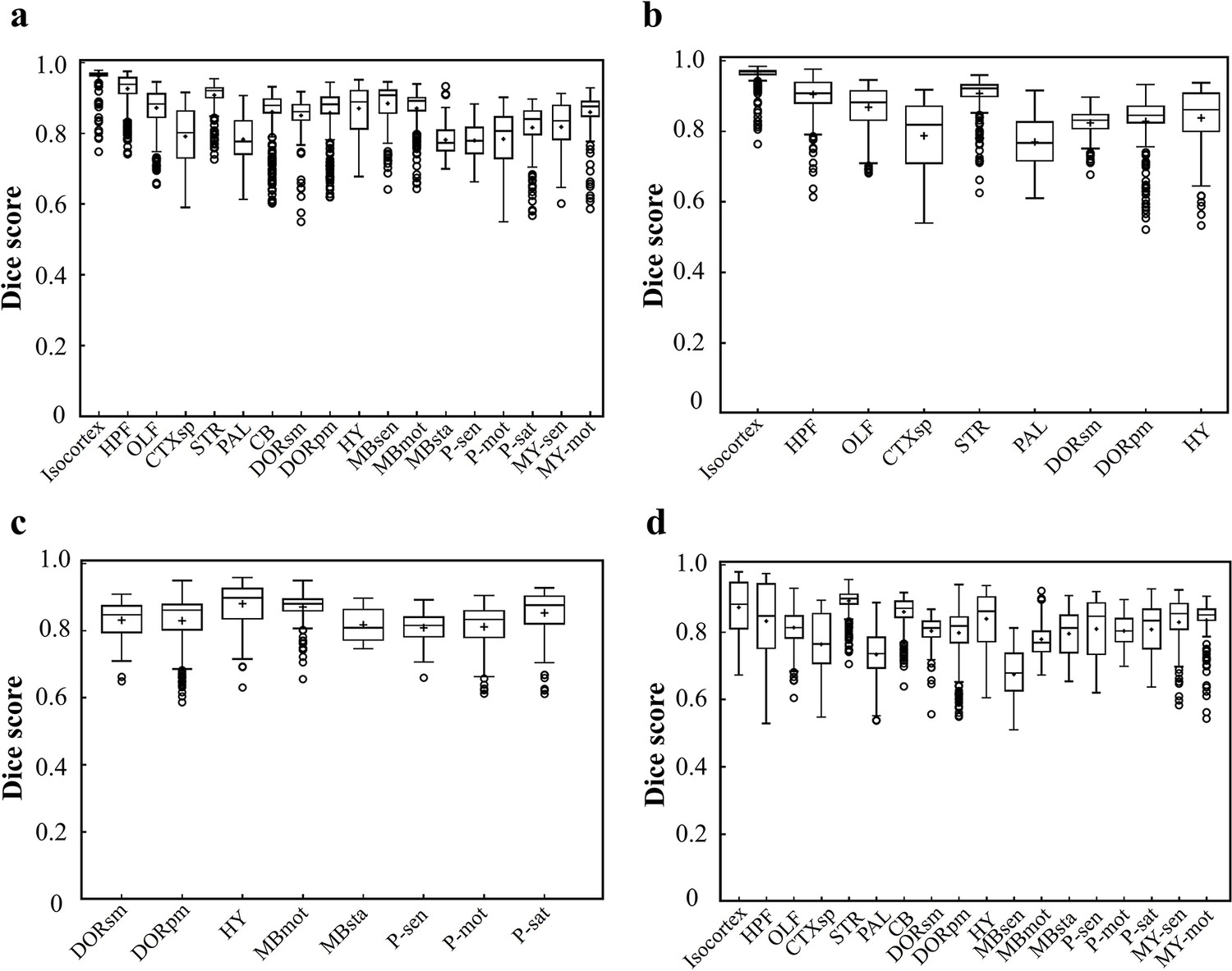
Dice scores of the DNN-segmented regions in three new types of incomplete brains.
These three incomplete brains, also shown in Figure 4c–e, all look different with the training data modes. Thereby, we can test the real inference capability of the trained DNN for segmenting unfamiliar data. (a) Dice scores of 18 DNN-segmented regions in right hemisphere. The ground-truth references used for calculation are the results obtained by bi-channel registration plus manual correction. The averaged median value of Dice scores was 0.86, with maximum value of 0.965 at Isocortex and minimum value of 0.78 at P-sen. (b) Dice scores of 10 DNN-segmented regions in an irregular cut of half telencephalon. The averaged median value of Dice scores was 0.87, with maximum value of 0.97 at Isocortex and minimum value of 0.771 at PAL. (c) Dice scores of seven DNN-segmented regions in a small random cut of brain. The averaged median value of Dice scores was 0.86, with maximum value of 0.958 at Isocortex and minimum value of 0.745 at PAL.
-
Figure 5—figure supplement 1—source data 1
Source data file for Figure 5—figure supplement 1.
- https://cdn.elifesciences.org/articles/63455/elife-63455-fig5-figsupp1-data1-v3.zip
Figure 5—figure supplement 2
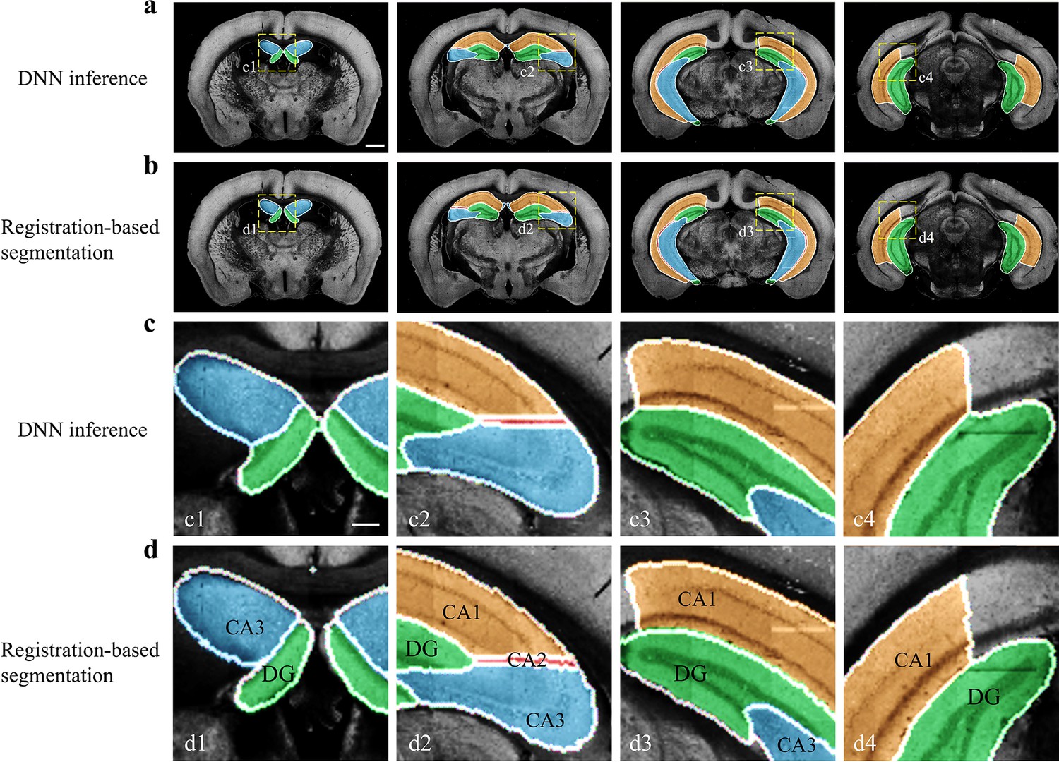
Performance of DNN inference for segmenting fine sub-regions specifically in the hippocampus.
Four coronal planes containing hippocampal sub-regions of CA1, CA2, CA3, and the DG are shown and compared to the bi-channel registration results. (a, b) Color-rendered segmentations of CA1, CA2, CA3, and DG by network inference and bi-channel registration (with manual correction), respectively. Scale bar, 1 mm. (c, d) Magnified views of the selected small regions (boxes) revealing the highly similar segmentation results by DNN inference and bi-channel registration. Scale bar, 250 μm. The averaged median value of Dice scores was 0.878, with maximum value of 0.96 at CA1 and minimum value of 0.70 at CA2.
Figure 5—figure supplement 3
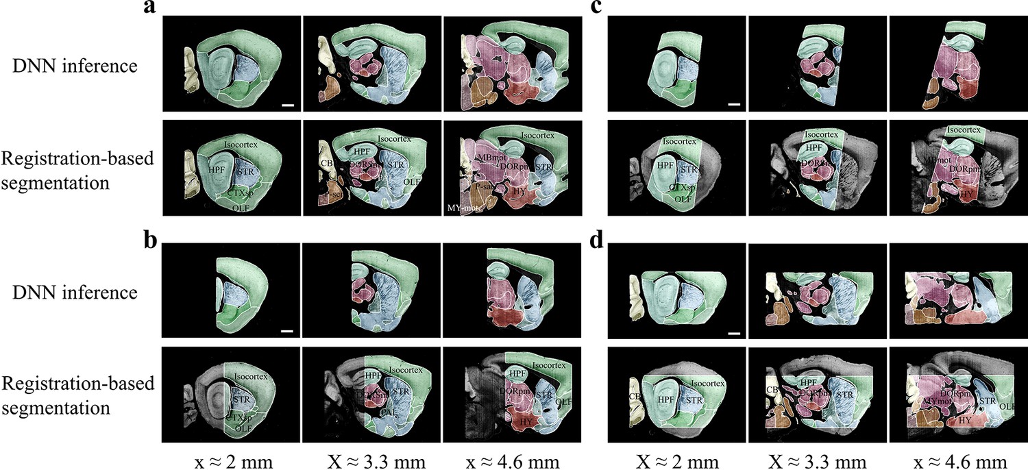
Accuracy comparison between DNN-based and registration-based brain segmentation.
We test the accuracy of DNN-inference-based segmentation through comparison with bi-channel registration results (after manual correction). An entire STP brain and three types of cropped incomplete brain regions, which are the same modes of data selected for network training (Figure 2b), are included for performance validation, with results shown in (a–d). In the comparative analysis of each group of data, we showed the same three sagittal planes (20 μm interval) segmented by DNN inference (upper row) and bi-channel registration (lower row). Eighteen segmented regions compared in the four modes of brain data (Isocortex, HPF, OLF, CTXsp, STR, PAL, CB, DORpm, DORsm, HY, MBsen, MBmot, Mbsta, P-sen, P-mot, P-sat, MY-sen, MY-mot) have widely verified the sufficient segmentation accuracy by our DNN inference. Scale bar, 1 mm.
Figure 5—figure supplement 4
Dice scores of the DNN-segmented regions in abovementioned four types of brains.
Data plots in a, b, c, d correspond to segmentation results shown in a, b, c, d, respectively. The average median value of Dice scores for most of the individual regions in all four brain modes are above 0.8, for example, Isocortex (~0.941), HPF (~0.884), OLF (~0.854), STR (~0.908), thereby showing a high inference accuracy for most of brain regions. At the same time, the performance of the network for segmenting PAL (~0.761) and MBsta (~0.799) regions remain limited, possibly owing to the large structure variation of these two regions as we move from the lateral to medial images across the sagittal plane.
-
Figure 5—figure supplement 4—source data 1
Source data file for Figure 5—figure supplement 4.
- https://cdn.elifesciences.org/articles/63455/elife-63455-fig5-figsupp4-data1-v3.zip
Figure 5—figure supplement 5
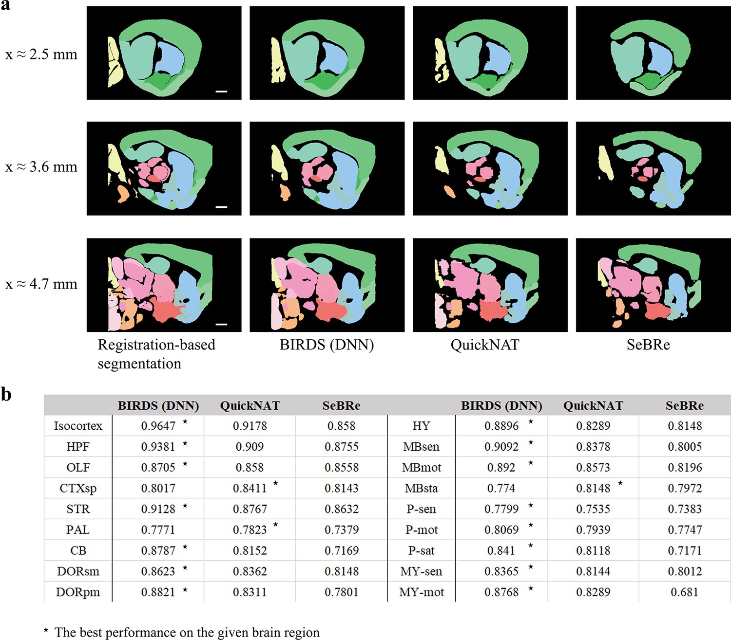
Comparison of the performance of DNN inference by three deep learning-based brainregion segmentation techniques, QuickNAT, SeBRe and our BIRDS (DNN).
(a) BIRDS (Bi-channel registration) and DNNs-inference-based segmentation results of an entire STP brain. Scale bar, 1mm. In the comparative analysis of each method, we showed the same three sagittal planes (20-μm interval) segmented by DNN inference (BIRDS, QuickNAT, SeBRe) and bi-channel registration. Eighteen regions (Isocortex, HPF, OLF, CTXsp, STR, PAL, CB, DORpm, DORsm, HY, MBsen, MBmot, Mbsta, P-sen, P-mot, P-sat, MY-sen, MY-mot ) segmented by the three deep learning-based methods have widely verified the sufficient segmentation accuracy by DNN inference. In most of brain regions the performance of BIRDS (DNN) is the best among the three (*), except CTXsp, PAL, and MBsta (QuickNAT is better than BIRDS (DNN) and SeBRe).
Videos
Video 1
Displays the 3D digital atlas.
Video 2
Shows the arborization of 5 neurons in 3D map space.
Additional files
-
Supplementary file 1
Data size, memory cost and time consumption at different BIRDS stages for processing 180 GB STPT and 320 GB LSFM datasets.
- https://cdn.elifesciences.org/articles/63455/elife-63455-supp1-v3.xlsx
-
Supplementary file 2
Details of training dataset and test dataset for coarse and fine DNN segmentations.
- https://cdn.elifesciences.org/articles/63455/elife-63455-supp2-v3.xlsx
-
Supplementary file 3
The median values corresponding to Figure 2d–f.
- https://cdn.elifesciences.org/articles/63455/elife-63455-supp3-v3.xlsx
-
Transparent reporting form
- https://cdn.elifesciences.org/articles/63455/elife-63455-transrepform-v3.docx
Download links
A two-part list of links to download the article, or parts of the article, in various formats.
Downloads (link to download the article as PDF)
Open citations (links to open the citations from this article in various online reference manager services)
Cite this article (links to download the citations from this article in formats compatible with various reference manager tools)
Bi-channel image registration and deep-learning segmentation (BIRDS) for efficient, versatile 3D mapping of mouse brain
eLife 10:e63455.
https://doi.org/10.7554/eLife.63455


