Live imaging and biophysical modeling support a button-based mechanism of somatic homolog pairing in Drosophila
- Department of Molecular and Cell Biology, University of California, Berkeley, United States
- Department of Physics, University of California, Berkeley, United States
- Biology Department, Bowdoin College, United States
- Univ Grenoble Alpes CNRS, Grenoble INP, TIMC-IMAG, France
- Biophysics Graduate Group, University of California, Berkeley, United States
- Université de Lyon, ENS de Lyon, Univ Claude Bernard, CNRS, Laboratory of Biology and Modeling of the Cell, France
- Institute for Quantitative Biosciences-QB3, University of California, Berkeley, United States
Figures
Figure 1
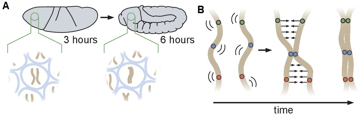
Schematic of homologous chromosome pairing in somatic cells in D. melanogaster.
(A) Over the course of embryonic development, homologous chromosomes pair along their lengths. (B) Button model for homolog pairing in which each chromosome carries a series of sites that have affinity for the same site on its homologous chromosome.
Figure 2 with 6 supplements
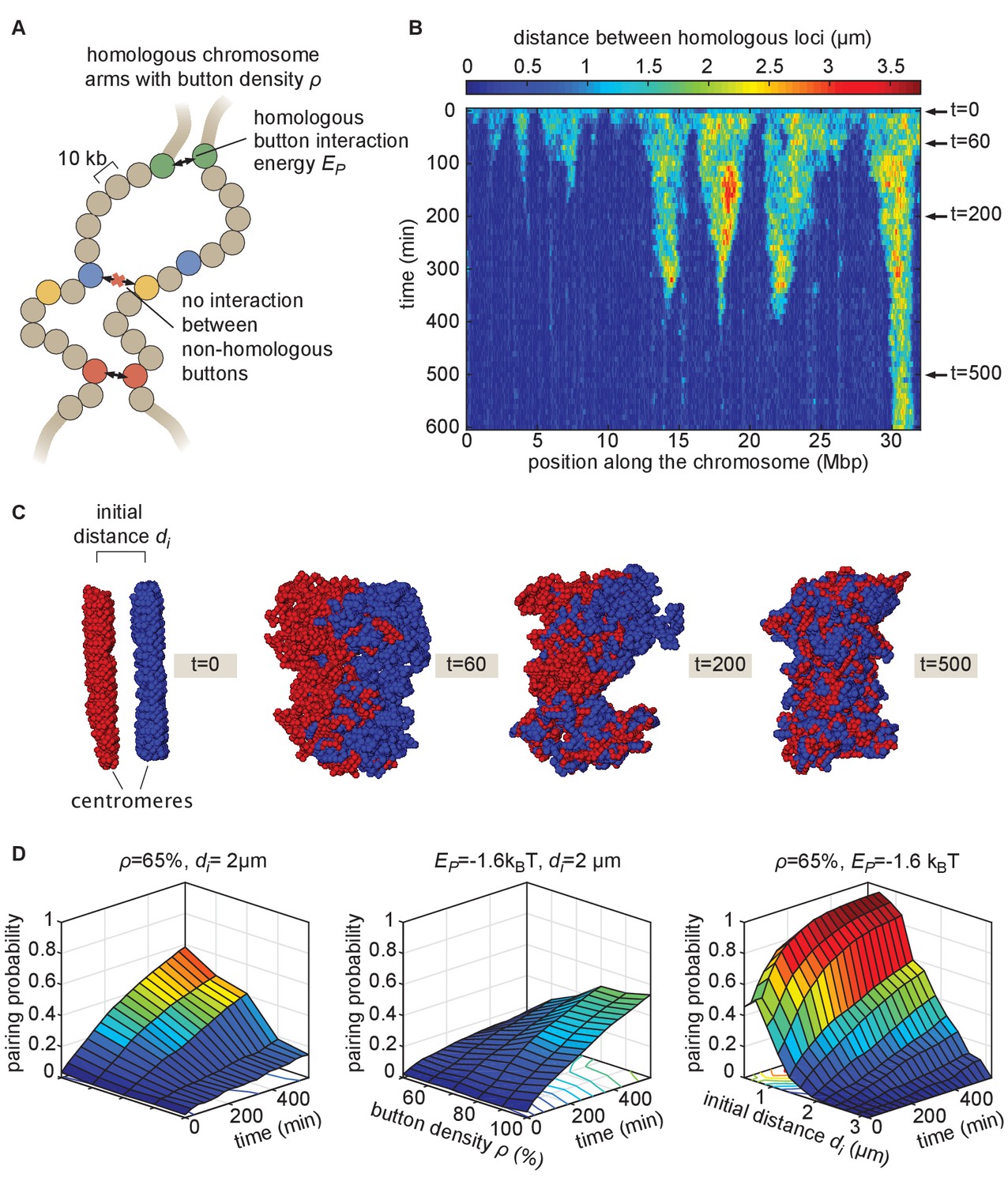
The homologous button model.
(A) Pairing between homologous chromosomes is assumed to be driven by specific, short-range attractive interactions of strength between certain homologous regions, named buttons. Each 10-kb monomer in the simulation corresponds to one locus. (B) Kymograph of the time evolution of the distances between homologous regions predicted by the model in one representative simulated stochastic trajectory for a button density of ρ = 65%, an interaction strength of = −1.6kBT, and an initial distance . See Figure 2—figure supplement 1 for other examples for various values. (C) Snapshots of the pair of homologous chromosomes at various time points along the simulation in (B) (see also Figure 2—video 1 and 2). (D) Predicted average pairing probability between euchromatic homologous loci (considered as paired if their relative distance ) as a function of time and of the strength of interaction (left), the button density ρ (center), and the initial distance between homologous chromosomes (right).
Figure 2—figure supplement 1
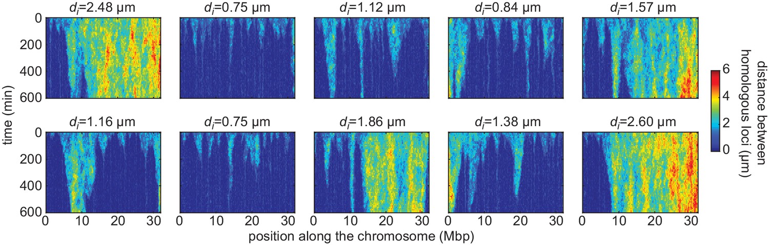
Simulated time evolution of distance between homologous loci.
Examples of kymographs of the time evolution of the distances between homologous regions predicted by the model in several simulated stochastic trajectories with different initial distances di for a button density of ρ = 65% and an interaction strength of = −1.6kBT. Pairing operates via a ‘zippering’ mechanism: as one pair of homologous loci becomes stably paired, the pairing of adjacent buttons is facilitated, leading to the ‘spreading’ of pairing along the chromosome (flame-like patterns in the kymographs). For smaller initial distances, pairing is faster and more efficient.
Figure 2—figure supplement 2
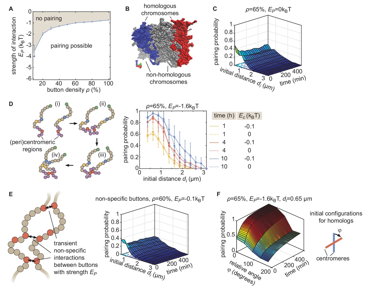
Properties of the button model.
(A) Phase diagram of parameter ranges resulting in simulations compatible (white area) and incompatible (gray area) with pairing, starting from favorable initial homologous chromosome configurations (aligned chromosomes with µm, as in Figure 2C). (B) Representative simulation snapshot for ρ = 65% and kT. When homologous chromosomes (red and blue monomers) are initially distant, steric hindrance by other chromosomes (gray monomers) may prevent pairing. (C) Behavior in the absence of specific interaction ( = 0) in the homologous button model. Predicted average pairing probability between euchromatic homologous loci (considered as paired if distance ) as a function of time and the initial distance between homologous chromosomes. (D) Impact of HP1-mediated interaction between (peri)centromeric regions. (Left) Pairing between chromosomes that are initially distant (i) is facilitated and accelerated by the non-specific interactions between centromeric regions that lead to the clustering (ii) of HP1 regions. This clustering facilitates the pairing of homologous buttons located in centromeric regions (iii) and the subsequent pairing via the zippering process of nearby euchromatic regions (iv). (Right) Predicted average pairing probability between euchromatic homologous loci (considered as paired if distance ) as a function of the initial distance between homologous chromosomes at 1 hr, 4 hr, and 10 hr for ρ = 65% and = −1.6kT in the presence (, full lines) or absence (, dashed lines) of interactions between (peri)centromeric regions. Even for large initial distances (), we observe a weak but significant amount of pairing in the euchromatic regions. These predictions are consistent with DNA-FISH experiments at various loci, suggesting an average higher pairing probability in heterochromatic loci during embryogenesis (see Figure 1 and Sup. Fig. 2 in Erceg et al., 2019). (E) The non-specific button model. To verify whether a non-specific button model can lead to global pairing, we relaxed the homologous model such that buttons may interact with any other buttons in the nucleus (left). In this model, the energy of a given configuration was described by.
We varied ρ from 10 to 100% and from −0.025 to −4kT, one realization of which is shown here (right), without observing any global pairing of homologous chromosomes. Other parameters were as in the homologous button model (see Materials and methods of the main text). Contacts preferentially form between buttons belonging to the same chromosome, or more weakly, between buttons of different chromosomes but not necessarily between homologous loci. (F) Effect of the relative initial orientation between homologs. Predicted average pairing probability between euchromatic homologous loci (considered as paired if distance ) as a function of time and the angle between the initial configurations of homologs (see inset), for an initial distance between the centers of mass of homologous chromosomes . We see that lower relative angles lead to more efficient pairing, with Rabl-like configurations corresponding to .
Figure 2—figure supplement 3
Large-scale correlations in pairing probabilities.
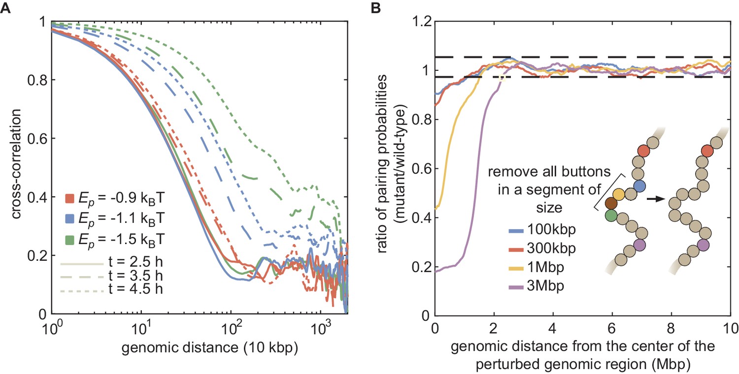
(A) Cross-correlation of the simultaneous pairing status of two loci separated by a given genomic distance computed for different values (ρ = 80%) at different simulated developmental times. This cross-correlation mathematically corresponds to the correlation between a binary variable defining the pairing status at a given time t of a pair of homologous loci at position i (= 0 if unpaired and = 1 if paired) and the same variable but for another pair at position j, and averaged over all the possible couples of pairs (i, j) separated by the same genomic distance. Due to the polymeric nature of the chromosome, nearby loci (distant by less than 500kbp) remain significantly correlated even for weak . However, while this correlation remains constant during development when pairing remains globally very low (red lines), the genomic range where loci tend to be correlated grows with developmental time as global pairing increases (blue and green lines). For example, for a scenario compatible with the experimental data (, blue lines), sites distant by more than 2 Mbp are highly correlated 2 hr after the beginning of the simulations (dotted line). (B) Investigation of the role of local perturbations of the button density on pairing efficiency. For parameters compatible with the experimental data (ρ = 80%, ), we simulated mutant situations where all the buttons in a given chromosomal segment are removed and calculated their pairing dynamics. Full lines represent the ratio between the long-time (between 6 and 8 hr after the beginning of the simulations) local pairing probability in the mutant and the corresponding quantity in the wild-type situation (i.e., without button removal) as a function of the genomic distance to the central monomer of the perturbed chromosomal segment for different sizes of the perturbation (100 kbp, 300 kbp, 1 Mbp, 3 Mbp). The black dashed lines represent the limit of a 99% confidence interval characterizing the ratio of the local pairing probability between two simulation replicas of the wild-type case. We observed that the local perturbation propagates to distant sites. Indeed, the pairing probability is significantly reduced (ratio below the lowest black dashed line) up to approximately 800 kbp to 1 Mbp from the border of the mutated region.
Figure 2—figure supplement 4
The combinatorial and large button models.
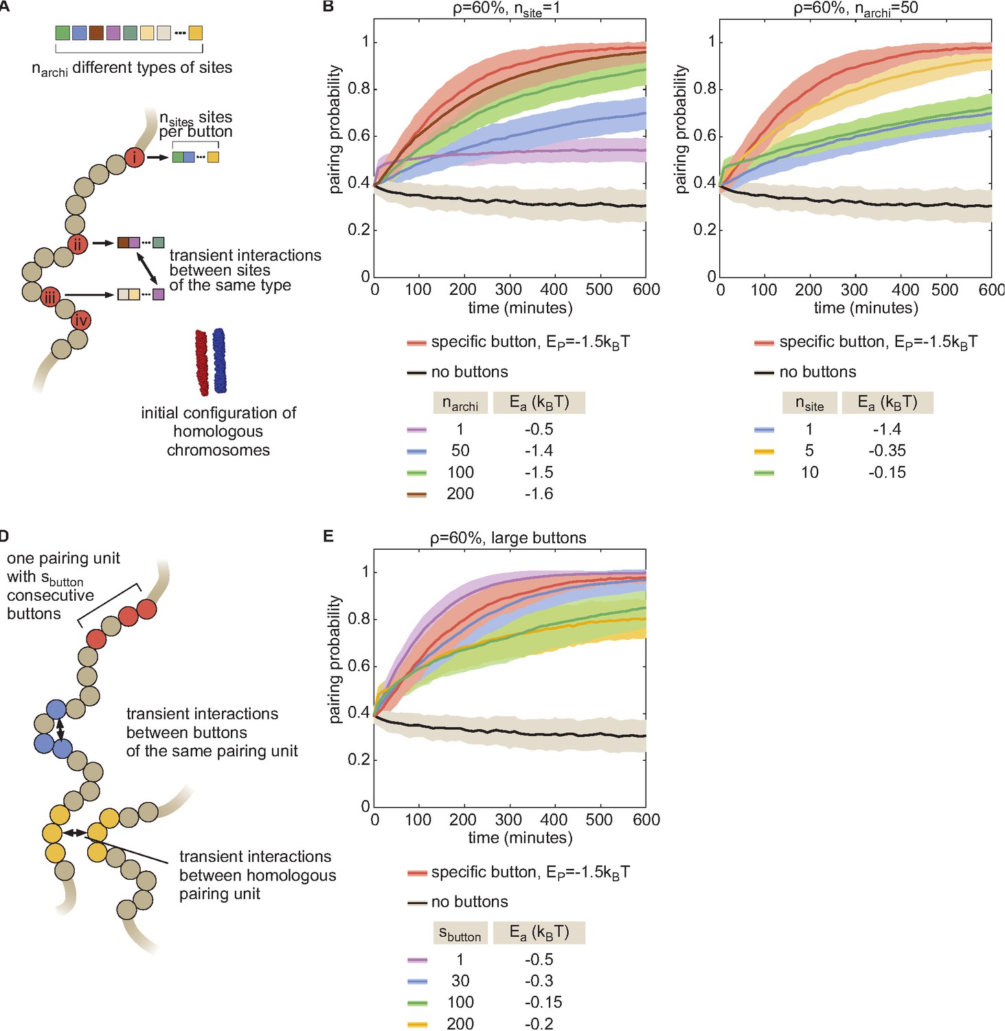
(A) To investigate the possible nature of buttons, we developed a more general model in which buttons are made of nsite binding sites for specific architectural proteins. Every site is occupied by one type of architectural proteins randomly chosen among narchi types. Two buttons may interact if they have common binding sites for some architectural proteins. The energy of a configuration is given by.
with parameters defined as in Equation S1, being the number of common binding sites between buttons (chr,i) and (chr’,j), and being the strength of interaction between binding sites bound to the same architectural proteins. Homologs share the same pattern of binding sites, that is if chr and chr’ are homologous and if i is a button. For example, the case nsite = 1, narchi = 1 ( = 1 ,) corresponds to the non-specific button model described in Figure 2—figure supplement 2E. To simplify and to avoid potential issues arising from periodic boundary conditions, we focused on favorable situations for pairing where homologs are initially aligned and close to each other (~640 nm between their respective centers of mass, see inset in A) and where the monomers evolve in a closed box (rigid wall conditions). Using this model, we first investigated how specific a button should be in order to lead to pairing. We fixed nsite = 1 and varied narchi and for a button density of 60%. In these cases, narchi represents the number of button types. In (B), we plotted, for each narchi, the time evolution of the average pairing probability between homologous sites (paired if distance ) for the value that leads to maximal pairing. As a point of comparison, we also plotted the corresponding curves in the absence of buttons (black line) and for the homologous button model investigated in the main text (red line) for the value (–1.5kT) consistent with experiments at the corresponding button density. We observed that as narchi increases (as the buttons become more specific) the pairing efficiency increases. The full specific model (red) becomes well approximated by our combinatorial button model for narchi > 200, i.e., when the number of buttons for one type is less than 10 per chromosome at 10kbp resolution. This suggests that pairing needs a significant degree of specificity via a large number of button types but each button type may be present in a small amount. However, we consider it unlikely that there are enough different architectural proteins in Drosophila to reach such single-site specificity. A possibility to increase specificity from a small number of proteins is to allow more than one binding site per button (nsite > 1). The number of different buttons is then (nsite)!/[(narchi-nsite)!(nsite)!]. In (C), we fixed narchi = 50, an upper maximal number of architectural proteins in flies, and varied nsite. For each nsite, we plotted the pairing probability for the value that leads to maximal pairing. We observed that there exists an optimal number of sites (here ~5) for which the pairing is close to the one obtained with the homologous button model. This corresponds to a value that leads to a large diversity of buttons while maintaining a low number of spurious interactions between non-homologous buttons, which is of the order of nsite/narchi~0.1. (D–E) In the main text, we assumed that the size of a specific button corresponded to one monomer in our simulations (10 kbp). Recently, Viets et al., 2019 suggested that homologous TADs (average size ~100 kbp [Haddad et al., 2017]) may be the basic units of pairing. (D) To test this hypothesis, we developed a variant model that assumed that one pairing unit is composed by consecutive buttons along the genome. These buttons can interact specifically with each other and with their homologs at an interaction energy . For example, the situation depicted in the main text corresponds to . Formally this model is equivalent to the combinatorial model with = 1 and with narchi = (total number of buttons)/ where buttons of the same type were placed consecutively along the chain (instead of randomly in the combinatorial model). As in (A–C), we simulated favorable situations where homologs are initially aligned and close to each other and where the monomers evolve in a closed box, using the same Hamiltonian as the combinatorial model. (E) Time evolution of the average pairing probability between homologous sites (paired if distance ) for different values and the value that leads to maximal pairing for a fixed global button density of 60%. We observed that the level of pairing obtained for the full specific button model at an interaction strength compatible with experiments (red) can only be achieved if is smaller than ~40–50 buttons. This would correspond to pairing units of maximal size of about 750 kbp. For larger units, cis interactions (between buttons of the same unit on the same chromosome) dominate over trans interactions (between homologous buttons of the same unit) leading to less efficient pairing. TADs, that would correspond to ~ 5–15, are therefore possible pairing units compatible with pairing.
Figure 2—video 1
Polymer simulations of homologous pairing.
Example of a 4-hr numerical simulation of the homologous button model (ρ = 60%, = −1.6 kBT) with frames taken every 30 s. The movie focuses on one pair of homologs (red and blue polymers). Orange and cyan parts of these chains represent their (peri)centromeric regions. Surrounding transparent light gray chains represent the periodic boundary images of the simulated chains. The scale bar is 1 µm. Homologous loci in closed contact (distance < 200 nm) are colored in green. Initially, chromosomes are randomly placed in a Rabl-like configuration. Then, they decompact and dynamically evolve in a crowded environment. First pairing events are diffusion-driven, followed by a spreading of pairing to nearest buttons via a zippering effect.
Figure 2—video 2
Polymer simulations of homologous pairing.
Same as in Figure 2—video 1 but taken from a different simulation run. The two pairs of homologs are highlighted (red/blue for one pair; purple/dark blue). Orange/cyan and pink/light blue parts of these chains represent their (peri)centromeric regions. Surrounding transparent light gray chains represent the periodic boundary images of the simulated chains. The scale bar is 1 µm. Homologous loci in closed contact (distance < 200 nm) are colored in green.
Figure 3 with 6 supplements

Live imaging of chromosomal loci provides dynamic single-locus spatiotemporal information about somatic homolog pairing.
(A) Schematic of the MS2 and PP7 nascent mRNA labeling scheme for live imaging of homologous loci. Expression of the stem loops is driven by UAS under the control of a GAL4 driver. (B) Snapshots at two time points from homologous chromosomal loci with one allele tagged with MS2 and one allele tagged with PP7 (top), negative controls consisting of non-homologous loci labeled with MS2 and PP7 (middle), and positive controls corresponding to a single reporter containing interlaced MS2 and PP7 stem loops on the same chromosome (bottom). Scale bars represent 1 µm. See also Figure 3—videos 1, 2, 3, 4. (C) Representative traces of the dynamics of the distance between imaged loci for unpaired homologous loci and the negative control showing how both loci pairs have comparable distance dynamics. (D) Representative traces of the dynamics of the distance between imaged loci for paired homologous loci and the positive control demonstrating how the distance between paired loci is systematically higher than the control. (E) Mean and standard deviation (SD) of the distance between reporter transgenes, where each data point represents a measurement over the length of time that the loci were imaged (ranging from approximately 10–50 min, depending on the duration of the movie and the length of time that a nucleus remained in the field of view, see Figure 3—figure supplement 1). The shaded region indicates the criterion used to define whether homologs are paired (mean distance < 1.0 µm, SD < 0.4 µm) based on the distribution of points where homologs were qualitatively assessed as paired (yellow and green points).
Figure 3—figure supplement 1
Experimental dynamics of inter-homolog distances used in Figure 3.
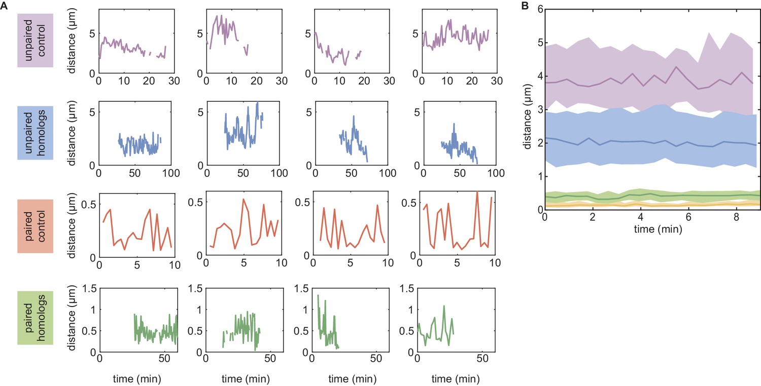
(A) Examples of individual traces in the unpaired (first row) and paired (third row) control cases, and when homologs are unpaired (second row) or paired (fourth row) for locus 38F. For the unpaired control, we monitored 21 trajectories of ~27 min in duration. For the paired control, 44 trajectories of ~10 min were imaged. For the unpaired homologs, 30 trajectories of 20–70 min were acquired. Finally, for paired homologs, 25 trajectories of 7–50 min were measured. (B) For each of these four categories, we computed the median (full lines) trajectory over ~10 min. The corresponding interquartile ranges are shown as shaded areas. Monitored trajectories longer than 10 min were divided into several 10 min long trajectories to enrich the statistics.
Figure 3—figure supplement 2
Homologous chromosome reporters inserted at the 53F genomic location.
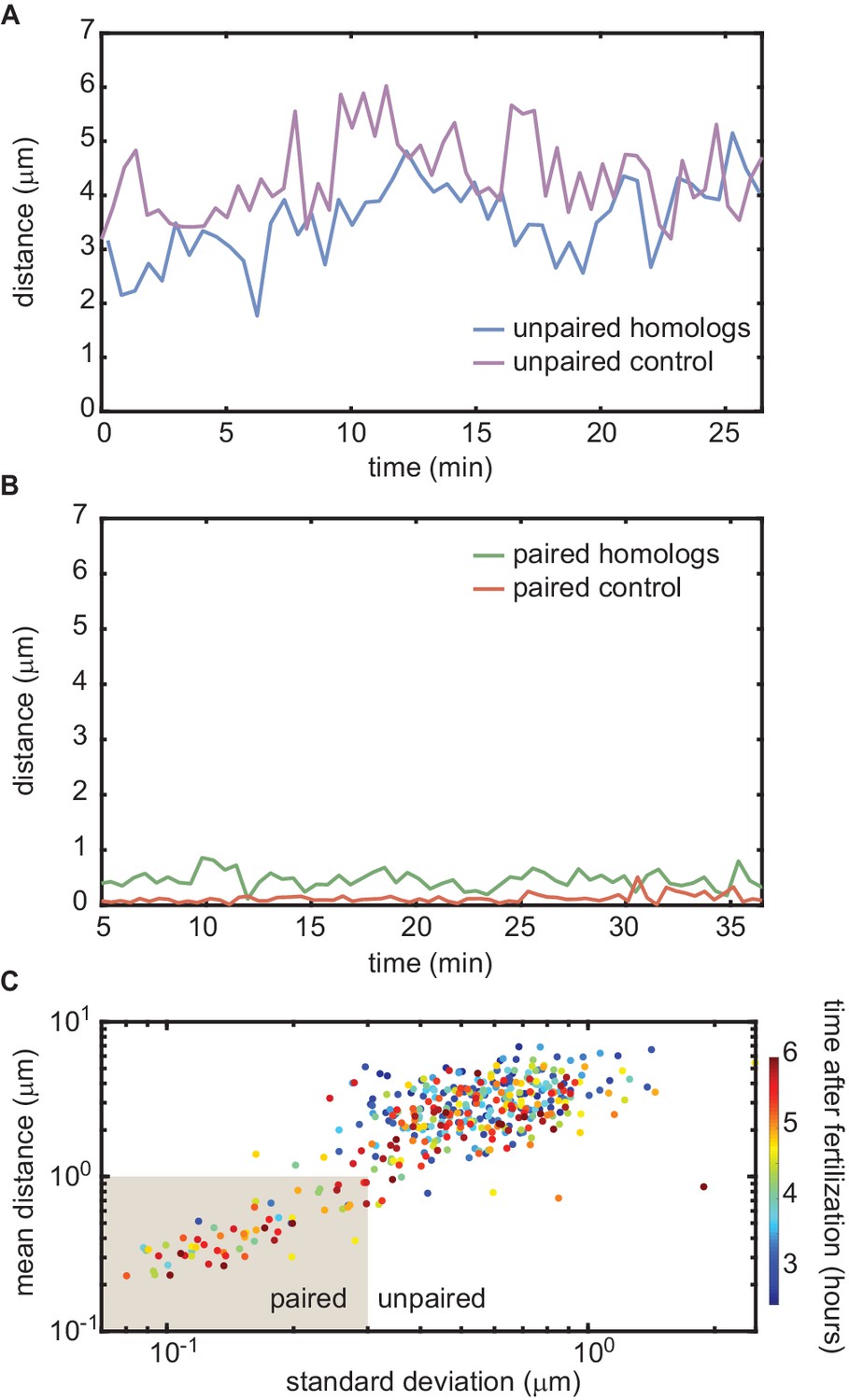
(A) Representative traces of the dynamics of the distance between imaged loci for unpaired homologous loci and the negative control. (B) Representative traces of the dynamics of the distance between imaged loci for paired homologous loci and the positive control. The traces in (A) and (B) are comparable to those measured at the 38F genomic location shown in Figure 3C,D. (C) Mean vs. standard deviation of the separation of each pair of homologous loci imaged in a single embryo over 6 hr of development (analyses of three embryos are combined). Each data point represents a 10 min window.
Figure 3—video 1
Representative confocal movie of a live Drosophila embryo (cell cycle 14 to gastrulation) in which MS2 and PP7 loops are integrated at equivalent positions on homologous chromosomes.
Examples of nuclei are highlighted whose loci display characteristic dynamics, including loci that do not pair (‘Unpaired’), loci that are already paired (‘Paired’), and loci that are observed transitioning from the unpaired to the paired state (‘Pairing’). Image stacks were taken roughly every 30 s and max-projected for 2D viewing.
Figure 3—video 2
Representative confocal movie of a live Drosophila embryo (roughly 4.5 hr old) in which MS2 and PP7 loops are integrated at equivalent positions on homologous chromosomes.
A greater proportion of nuclei show paired homologs relative to the earlier time point represented in Figure 3—video 1. Image stacks were taken roughly every 30 s and max-projected for 2D viewing.
Figure 3—video 3
Representative confocal movie of a live Drosophila embryo (roughly 5.5 hr old) in which MS2 and PP7 loops are integrated at various positions on homologous chromosomes (MS2 at position 38F and PP7 at position 53F) where we expect no pairing between transgenes.
Image stacks were taken roughly every 30 s and max-projected for 2D viewing.
Figure 3—video 4
Representative confocal movie of a live Drosophila embryo (cell cycle 14) in which MS2 and PP7 loops were interlaced in a single transgene on one chromosome at polytene position 38F to act as a positive control for pairing.
Both GFP and mCherry are co-localized to the same locus in all transcriptional loci. Image stacks were taken roughly every 30 s and max-projected for 2D viewing.
Figure 4 with 3 supplements
The homologous button model recapitulates the observed developmental dynamics of pairing.
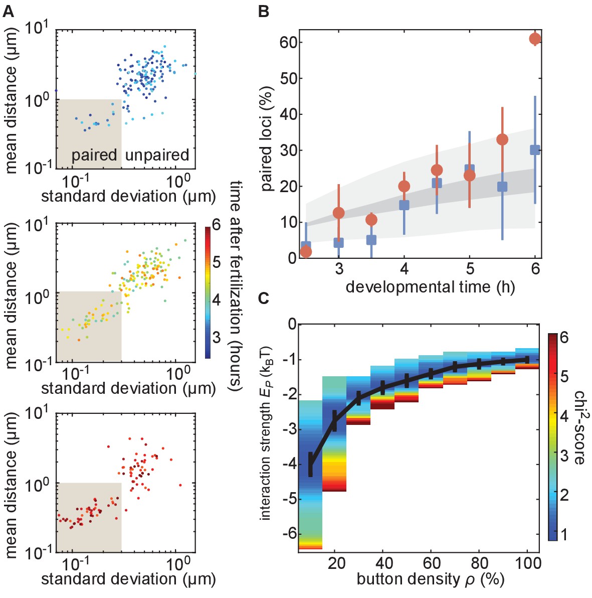
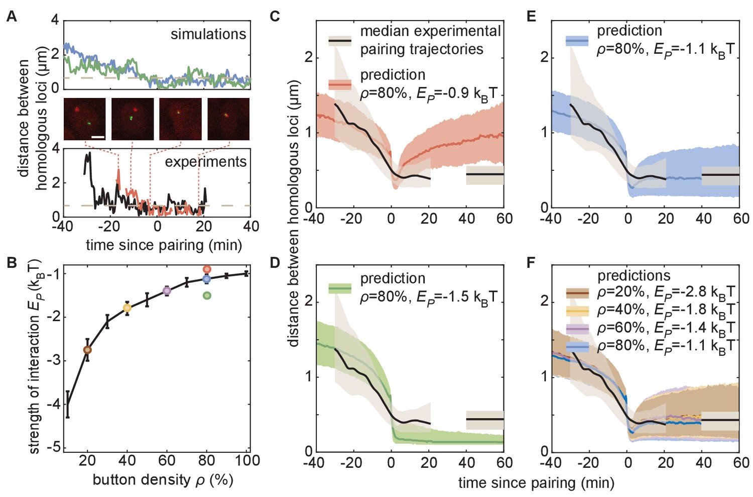
(A) Mean and SD of the separation of each pair of transgenes integrated at position 38F imaged in a single embryo over 6 h of development. Each data point represents a single nucleus over a 10-min time window, revealing the increase in the fraction of paired loci as development progresses. Data are separated into three plots for ease of visualization. (B) Nuclei from each time point were scored as “paired” if they fell within the shaded box in (A). Data were taken from three embryos each for transgenes at 38F (red) and 53F (blue) with error bars representing the standard error of the mean. For each button density ρ, we fitted the experimental pairing dynamics (Figure 4—figure supplement 2A). Gray shading provides the envelope of the best predictions obtained for each ρ (dark gray) and its SD (light gray). (C) Phase diagram representing, as a function of ρ, the value of (black line) that leads to the best fit between predicted and experimental developmental pairing dynamics. The predicted pairing strength is weaker than observed in the parameter space above the line, and stronger than observed below the line. Error bars represent the uncertainties on the value of that minimizes the chi2-score at a given ρ value.
Figure 4—figure supplement 1
Comparison of our pairing data to previous results.
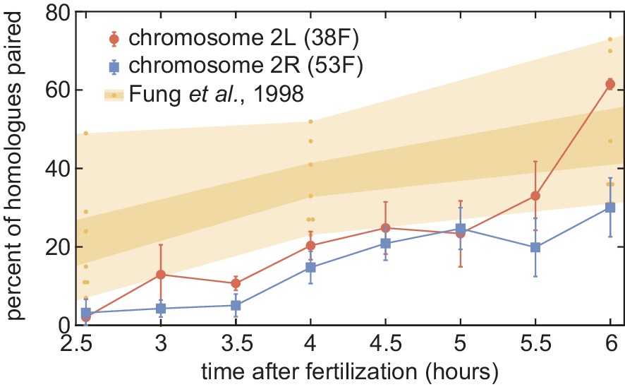
Pairing dynamics measured by live imaging at two chromosomal loci (red and blue points) as presented in Figure 4B. The progression of pairing observed in fixed embryos using DNA-FISH was obtained from Fung et al., 1998; yellow points represent the pairing measured at seven euchromatic loci on chromosome arm 2L at three time points, and yellow shading represents standard error (dark) and range (light). Our data is consistent with, but systematically lower than, the range of pairing observed in the prior study.
Figure 4—figure supplement 2
Establishing values for initial distance between homologous chromosomes via chromosome painting.
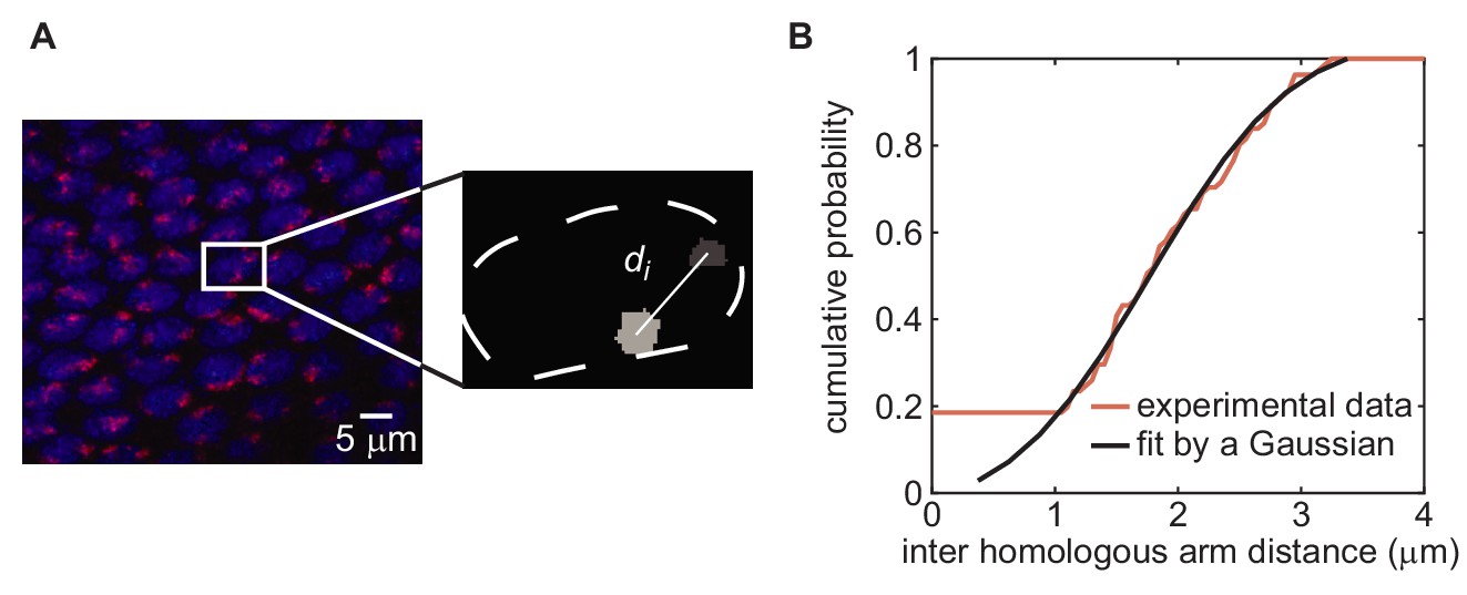
(A) Chromosome painting of chromosome arm 2L (red), carrying transgene location 38F, in an embryo in early cycle 14. Nuclei (blue) are stained with DAPI. Inter-homolog distances were determined by segmenting painted regions in 3D using ImageJ and measuring center-to-center distances (inset; see Materials and methods for details). Chromosome arm 2R, carrying transgene location 53F, was sampled in the same field of cells using a different fluorescent tag (not shown). (B) Distribution of inter-homologous arm distances measured from 48 nuclei in the image in (A) (red curve). Measurements from chromosome arms 2L and 2R were completely overlapping and therefore were combined. The curve is fitted by a Gaussian distribution (black curve, mean = 1.9, SD = 0.9).
Figure 4—figure supplement 3
Inference of developmental pairing dynamics.
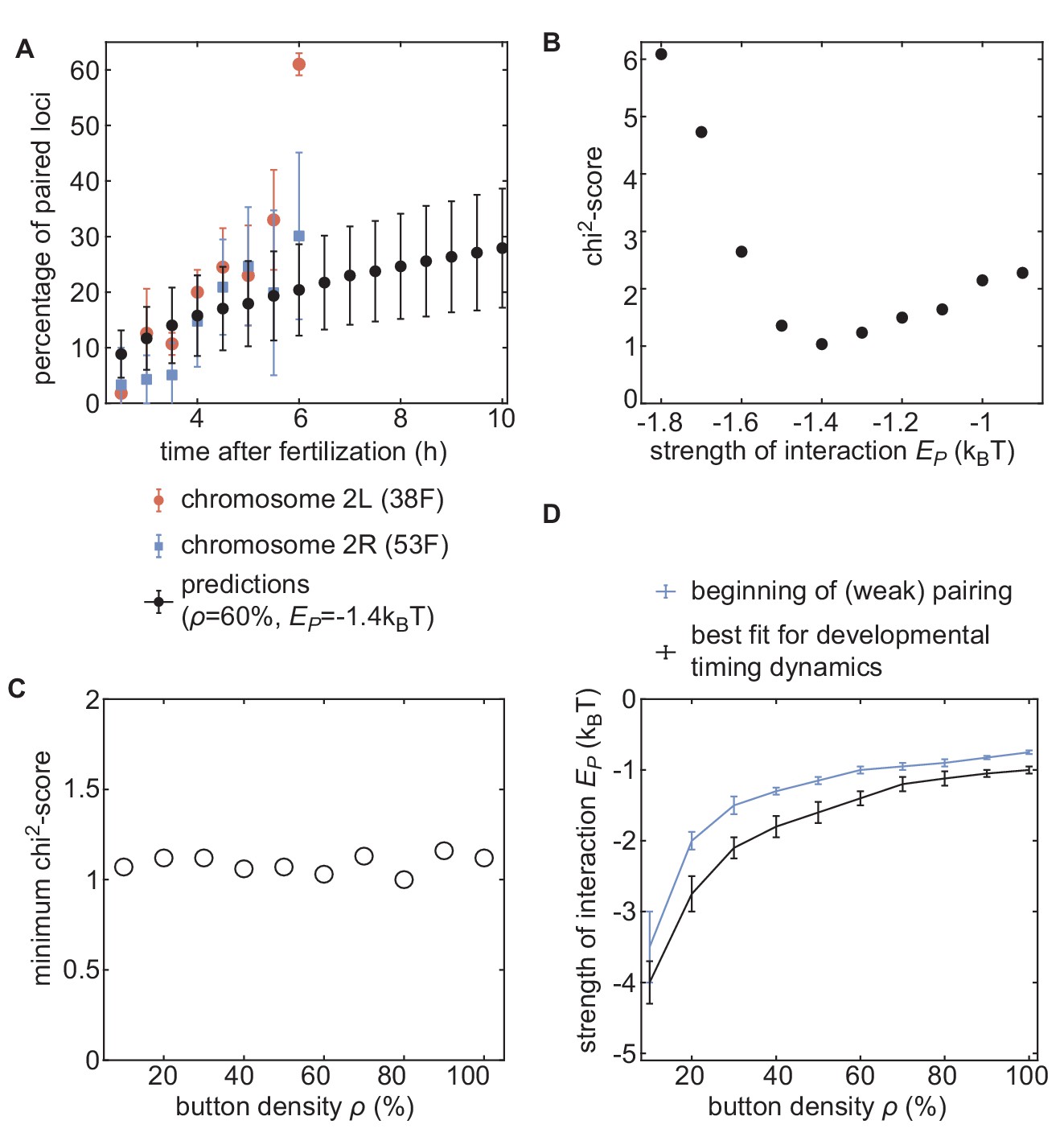
(A) Predicted time evolution of the mean pairing dynamics computed over all buttons in the simulation (black dots) for a distribution of initial inter-homolog distances given in Figure 4A and for ρ= 60% and = −1.4 kBT. Error bars in simulated data represent SD of the pairing dynamics computed over all the buttons (n = 3200), while error bars in experimental data represent the standard error of the mean (n = 3 embryos for each chromosomal position). The model can recapitulate the experimentally measured pairing dynamics. (B) Evolution of the chi2-score as a function of for ρ= 60%. For some values, we performed two sets of independent simulations. (C) The values of the minimum chi2-score obtained for all the investigated button densities are very similar, suggesting an equivalent predicting power for every ρ. (D) Phase diagram representing, for each button density ρ, the value of (black line) that leads to the best fit between predicted and experimental developmental pairing dynamics. The blue line stands for the weak pairing transition defined in Figure 2—figure supplement 2A.
Figure 5 with 3 supplements
The homologous button model predicts individual pairing dynamics.
(A) Examples of simulated (top) and experimental (bottom) pairing trajectories showing rapid transitions from the unpaired to the paired state. Simulations were carried out using ρ = 50% and . See also Figure 5—figure supplement 1. Scale bar is 2 μm. Dotted line in each graph represents our distance threshold for aligning pairing traces defined as the time point where the inter-homolog distance decreases below 0.65 µm for at least 4 min. (B) Parameter range inferred from pairing probability dynamics in Figure 4 (black line), and parameters used for the simulations in (C–F) (color points). (C–F) Median pairing dynamics obtained from individual pairing trajectories detected during our experiments (black lines) and simulations (colored lines). Traces are centered at the time of pairing (time = 0) as in (A). The long-term, experimentally measured inter-homolog distance is plotted as a straight black line at the right of each panel. The interquartile range of the distributions of distances between homologous loci are indicated by the shaded regions (n = 14 nuclei for experiments; n > 10,000 traces for simulations). Note that the experimental data were processed (Figure 5—figure supplement 1C) to smooth out the effect of small statistics (Figure 5—figure supplement 2C).
Figure 5—figure supplement 1
Experimental individual pairing dynamics.
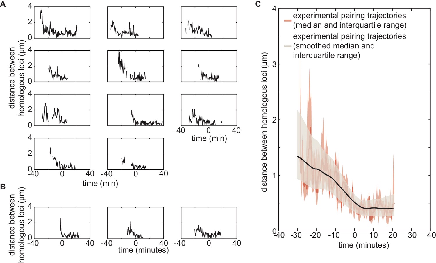
(A,B) Fast single-locus pairing dynamics illustrated by individual pairing traces detected for the experiments on locus 38F (A, n = 11) and locus 53F (B, n = 3) centered at the time of pairing (time = 0) defined as the time point where the inter-homolog distance decreases below 0.65 µm for at least 4 min. (C) From the 14 individual pairing trajectories observed experimentally, we estimated at each time point the median (dark red full line) and the interquartile range (light red shaded area) of the distribution of distances between homologous loci. The corresponding smoothed median is plotted in black, and the interquartile range (as in Figure 5 of the main text) is given by the gray shaded area. Smoothing was performed using the smooth function of Matlab (method = lowess, span = 40). In Figure 5—figure supplement 2C, we demonstrate the effect of very low statistics and of smoothing on the overall shape of the pairing dynamics using simulated data.
Figure 5—figure supplement 2
Impact of and small statistics on individual pairing dynamics.
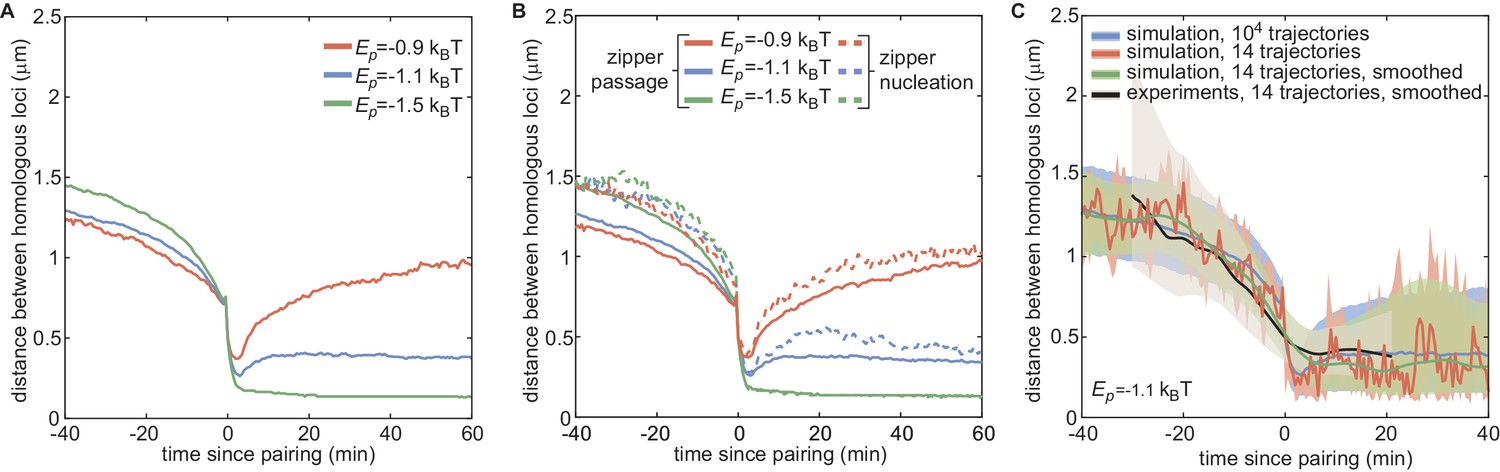
(A) Median pairing dynamics obtained from individual pairing trajectories detected during our simulations (colored lines) for ρ= 80% and different values of . Traces are centered at the time of pairing (time = 0) defined as the time point where the inter-homolog distance decreases below 0.65 µm for at least 4 min. While the main differences lie in the post-pairing period, with stronger leading to a smaller distance between paired homologous loci, weak changes in the pre-pairing dynamics can be observed with stronger leading to faster decay in the inter-homolog distance. (B) For the same trajectories obtained in (A), we clustered the individual pairing trajectories into two categories. First, trajectories corresponding to primary pairing events (dashed lines), that is when no other loci in a ±200kbp window become paired earlier. Second, all the other trajectories (full lines), that is when at least another locus in the neighborhood becomes paired earlier. When is strong enough to maintain pairing, the first category corresponds to the nucleations of zippers while the second to the passage of a zipper. As expected, the pre-pairing dynamics of primary events (dashed lines) do not depend on , reflecting the diffusion origin of these events. On the contrary, the passage events exhibit a faster pre-pairing dynamics for stronger energies, suggesting a more efficient zippering. (C) Impact of small statistics and smoothing on the median pairing dynamics. For ρ = 80% and , we randomly picked n = 14 trajectories (as in the experimental set) from our 10,0000 simulated trajectories, computed the median (orange line) and interquartile range (pink area) and smoothed them (green line and light gray area) with the same parameters used for the experimental curves (black line and gray area, see Figure 5—figure supplement 1C). In the pre-pairing dynamics, the small statistics (n = 14) and smoothing may slightly perturb the overall shape of the predicted median dynamics while still largely remaining within the interquartile range found using the full statistics (blue line and blue area).
Figure 5—video 1
Representative distance trajectory of two loci denoted as ‘pairing’ (plotted in the black experimental trace in Figure 5A) showing a rapid transition from large distances at earlier time points to smaller distances at later time points.
The trajectory is shown alongside movies of the nucleus and gastrulating embryo from which the distances were calculated to help visualize the speed at which this pairing occurs. Image stacks were taken roughly every 30 s and max-projected for 2D viewing.
Additional files
Download links
A two-part list of links to download the article, or parts of the article, in various formats.
Downloads (link to download the article as PDF)
Open citations (links to open the citations from this article in various online reference manager services)
Cite this article (links to download the citations from this article in formats compatible with various reference manager tools)
Live imaging and biophysical modeling support a button-based mechanism of somatic homolog pairing in Drosophila
eLife 10:e64412.
https://doi.org/10.7554/eLife.64412


