Hypoxia triggers collective aerotactic migration in Dictyostelium discoideum
- Institut Lumière Matière, UMR5306, Université Lyon 1-CNRS, Université de Lyon, France
- Institut Camille Jordan, UMR5208, Université Lyon 1-CNRS, Université de Lyon, France
- Graduate School of Biomedical Engineering, Tohoku University, Japan
- Institute of Fluid Science, Tohoku University, Japan
- Centre Léon Bérard, Centre de recherche en cancérologie de Lyon, INSERM 1052, CNRS 5286, Université Lyon 1, Université de Lyon, France
- Laboratoire de Biochimie et Pharmacologie, Faculté de médecine de Saint-Etienne, CHU de Saint-Etienne, France
- Graduate School of Engineering, Tohoku University, Japan
Figures
Figure 1 with 5 supplements
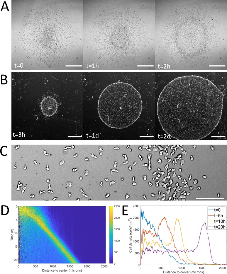
Formation and dynamics of a dense ring of cells after vertical confinement.
(A) Snapshots of early formation, scale bars: 500 μm. (B) Snapshots at longer times imaged under a binocular, scale bars: 1 mm. (C) Close up on a ring (band with a higher density on the right hand side) already formed moving rightward and showing different cellular shapes in the ring and behind it, scale bar: 100 μm. (D) Kymograph of cell density over 20 hr showing the formation and migration of the highly dense ring. (E) Cell density profiles in the radial direction at selected time points.
-
Figure 1—source data 1
Raw data for Figure 1.
- https://cdn.elifesciences.org/articles/64731/elife-64731-fig1-data1-v1.mat
Figure 1—figure supplement 1
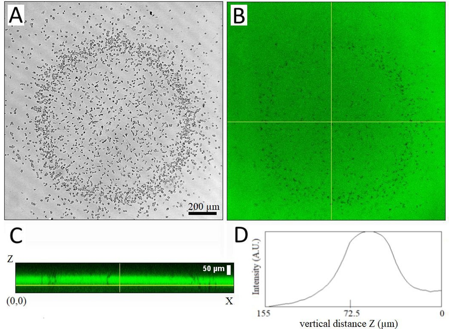
Measurement of the confinement height 105 min after covering a cell colony with ~1000 cells plated on plastic with a coverglass using.
(A-B) Confocal transmission and fluorescence XY images (slice 37) of a Z-stack from inside the plastic bottom of the well to the coverglass; (C) Side view XZ along the horizontal line in B. (D) Vertical intensity profile along Z (averaged over X). The Full width at half maximum (FWHM) is about 50 µm. Z-stacks were taken with a confocal microscope at 2.57 µm/slice using a 10x objective with a very small pinhole size (0.25 Airy), the fluorescence is due to fluorescein FITC added at 16 µM in HL5 medium.
Figure 1—figure supplement 2
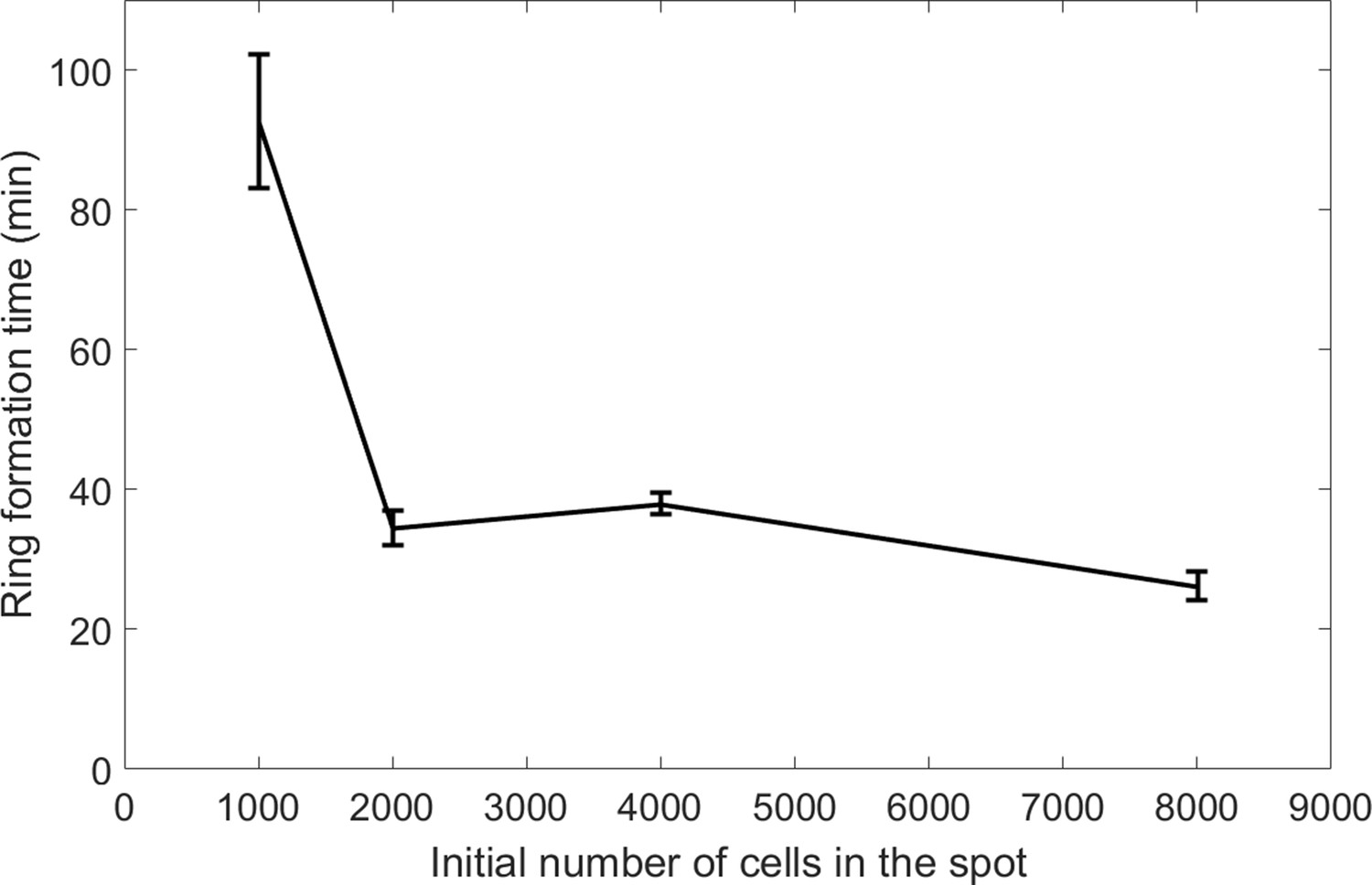
Ring formation time decreases with cell number.
Error bars represent std of n ≥ 4 independent experiments.
-
Figure 1—figure supplement 2—source data 1
Raw data for Figure 1—figure supplement 2.
- https://cdn.elifesciences.org/articles/64731/elife-64731-fig1-figsupp2-data1-v1.xlsx
Figure 1—figure supplement 3
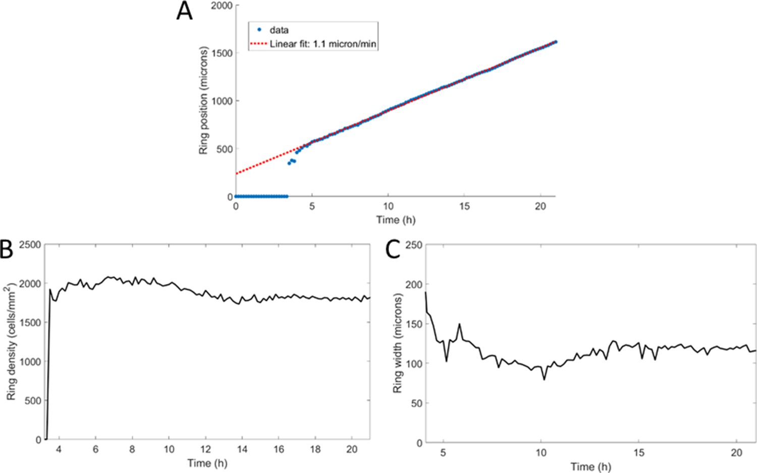
Morphological properties of a propagating ring.
(A) Position of the ring as a function of time with a linear fit yielding a speed of 1.1 μm/min. (B) Cell density within the ring as a function of time, starting after ring formation. (C) Ring width at half height as a function of time, after ring formation.
-
Figure 1—figure supplement 3—source data 1
Raw data for Figure 1—figure supplement 3.
- https://cdn.elifesciences.org/articles/64731/elife-64731-fig1-figsupp3-data1-v1.mat
Figure 1—figure supplement 4
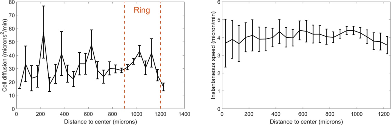
Effective cell diffusion constant and instantaneous speeds as a function of distance to the center.
Cell diffusion is defined as the squared of the migrated distance during a trajectory divided by 4 t with t the duration of that trajectory. Cells were tracked between t=9h and t=10h and orange dashed line represent the position of the ring at these times. Each point is the mean±std of cells within the given distance bin, n=2746 cells total.
-
Figure 1—figure supplement 4—source data 1
Raw data for Figure 1—figure supplement 4.
- https://cdn.elifesciences.org/articles/64731/elife-64731-fig1-figsupp4-data1-v1.mat
Figure 1—figure supplement 5
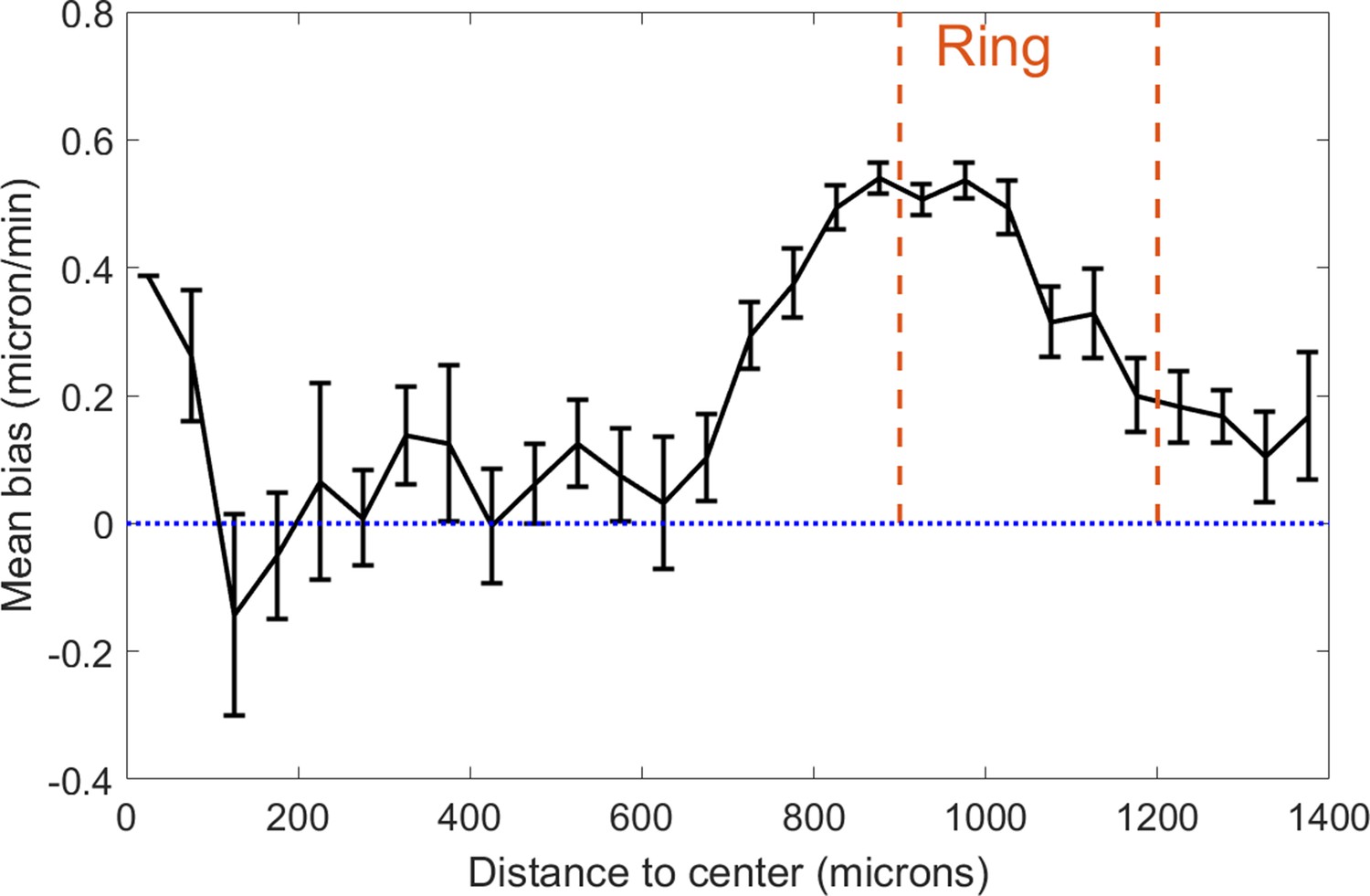
Cell velocity bias in the spot assay as a function of distance to the center.
This bias is defined as the projected speed in the radial direction. Each point is the mean±std of cells within the given distance bin, n=2211 cells total. Cells were tracked between t=9h and t=11h and orange dashed lines represent the positions occupied by the ring at these times. Dotted blue line is a guide for the eye representing a 0 bias, that is non-oriented motion.
-
Figure 1—figure supplement 5—source data 1
Raw data for Figure 1—figure supplement 5.
- https://cdn.elifesciences.org/articles/64731/elife-64731-fig1-figsupp5-data1-v1.mat
Figure 2 with 8 supplements
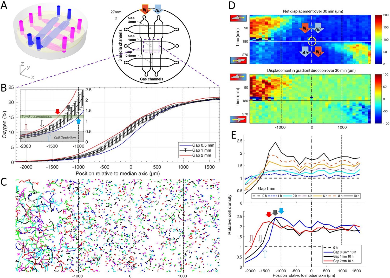
Dictyostelium single cells are attracted by an external O2 gradient when O2 level drops below 2%.
(A) Schemes of the new double-layer PDMS microfluidic device allowing the control of the O2 gradient by the separation distance (gap) between two gas channels located 0.5 mm above the three media channels and filled with pure nitrogen, and air (21% O2). (B) Measured O2 concentration profiles 30 min after N2-Air injection to the left and right channels respectively (0–21% gradient) as a function of the position along the media channel for the three gaps. Error bars (see Methods) are reported only for gap 1 mm for clarity. The inset shows the 0–2.5% region under the nitrogen gas channel (arrows, see E). (C) Trajectories lasting 1 hr between 3 hr and 4 hr after establishment of a 0–21% gradient. Cells are fast and directed toward the air side in the region beyond the −1000 µm limit (O2<2%). (D) Cell net displacement over 30 min (end to end distance, top kymograph) and 30 min displacement projected along gradient direction (bottom kymograph). Cells are fast and directed toward O2, where O2<2%, within 15 min after 0–21% gradient establishment at t=0. At t=180 min, the gradient is reversed to 21–0% by permuting gas entries. Cells within 15 min again respond in the 0–2% region. (E) Relative cell density histogram (normalized to t=0 cell density) as a function of the position along media channel. Top panel: long term cell depletion for positions beyond −1600 µm (O2<0.5%, see inset of B) and resulting accumulation at about −1200 µm for gap 1 mm channel. The overall relative cell density increase is due to cell divisions. Bottom panel: cell depletion and accumulation at 10 hr for the three gaps. The empty and filled arrows pointing the limit of the depletion region, and max cell accumulation respectively are reported in the inset of B.
-
Figure 2—source data 1
Raw data for Figure 2.
- https://cdn.elifesciences.org/articles/64731/elife-64731-fig2-data1-v1.xlsx
Figure 2—figure supplement 1
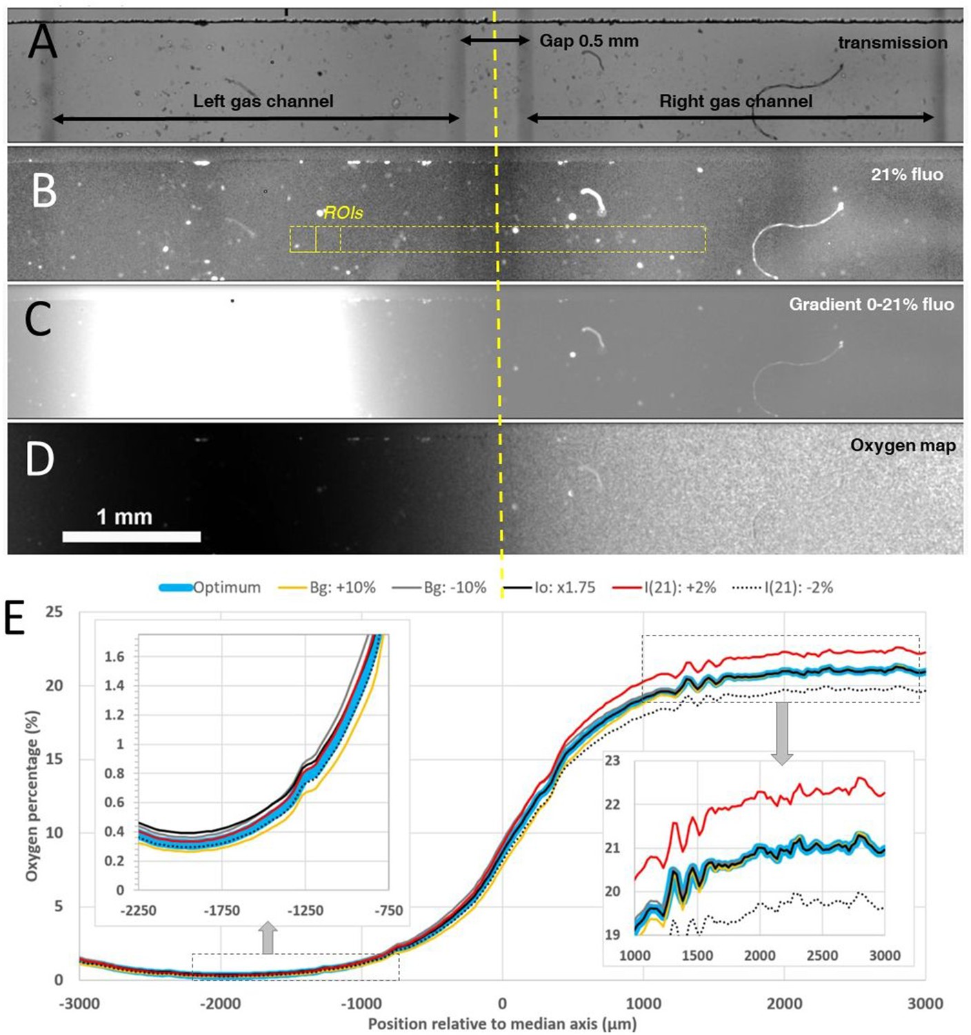
Oxygen profile measurements inside the microfluidic gradient generator device with a sensing film mounted on the bottom of the media channel.
(A-B) Transmission and homogeneous 21% O2 level fluorescence images of the media channel with gap 0.5 mm between the two gas channels. (C) Raw fluorescence image in presence of 0–21% gradient established by injecting pure N2 in the left gas channel and air in the right one (image was taken 30 min after the beginning of the gas injection). (D-E) Corresponding calculated O2 map and O2 profile. In D colors correspond to slight changes within the experimental uncertainty of the parameters used for the calculation (see text), insets correspond to the hypoxic (~0%) and normoxic (~21%) sides of the profile.
-
Figure 2—figure supplement 1—source data 1
Raw data for Figure 2—figure supplement 1.
- https://cdn.elifesciences.org/articles/64731/elife-64731-fig2-figsupp1-data1-v1.xlsx
Figure 2—figure supplement 2
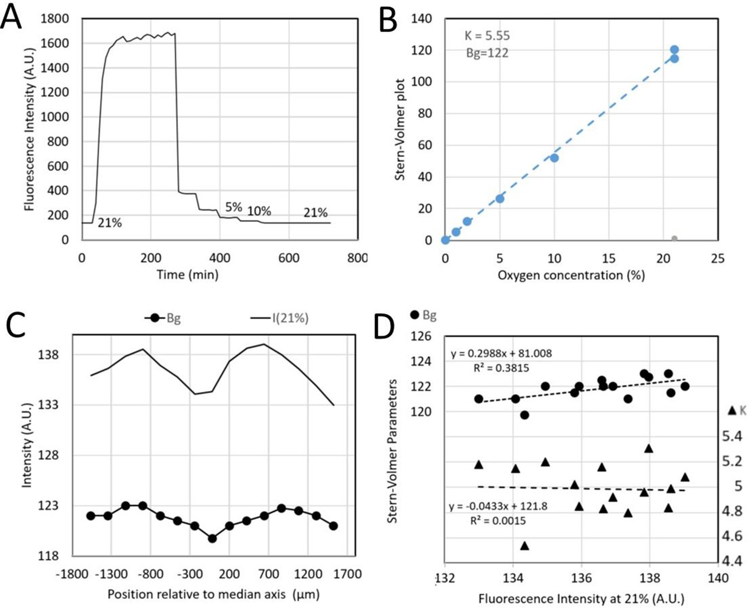
Typical calibration data of sensing films mounted on a microfluidic device.
(A) Fluorescence intensity changes when applying an oxygen concentration ramp with the concentration in each gas channel. (B) Corresponding Stern-Volmer plot (see text). (C) Measured intensity at 21% O2 level (solid line) and fitted background Bg (bullets) for different ROI locations depicted in yellow in Figure 2—figure supplement 1B. (D) Fitted Bg (bullets) and Stern-Volmer sensitivity parameter K (triangles) as a function of 21% O2 level intensity.
-
Figure 2—figure supplement 2—source data 1
Raw data for Figure 2—figure supplement 2.
- https://cdn.elifesciences.org/articles/64731/elife-64731-fig2-figsupp2-data1-v1.xlsx
Figure 2—figure supplement 3
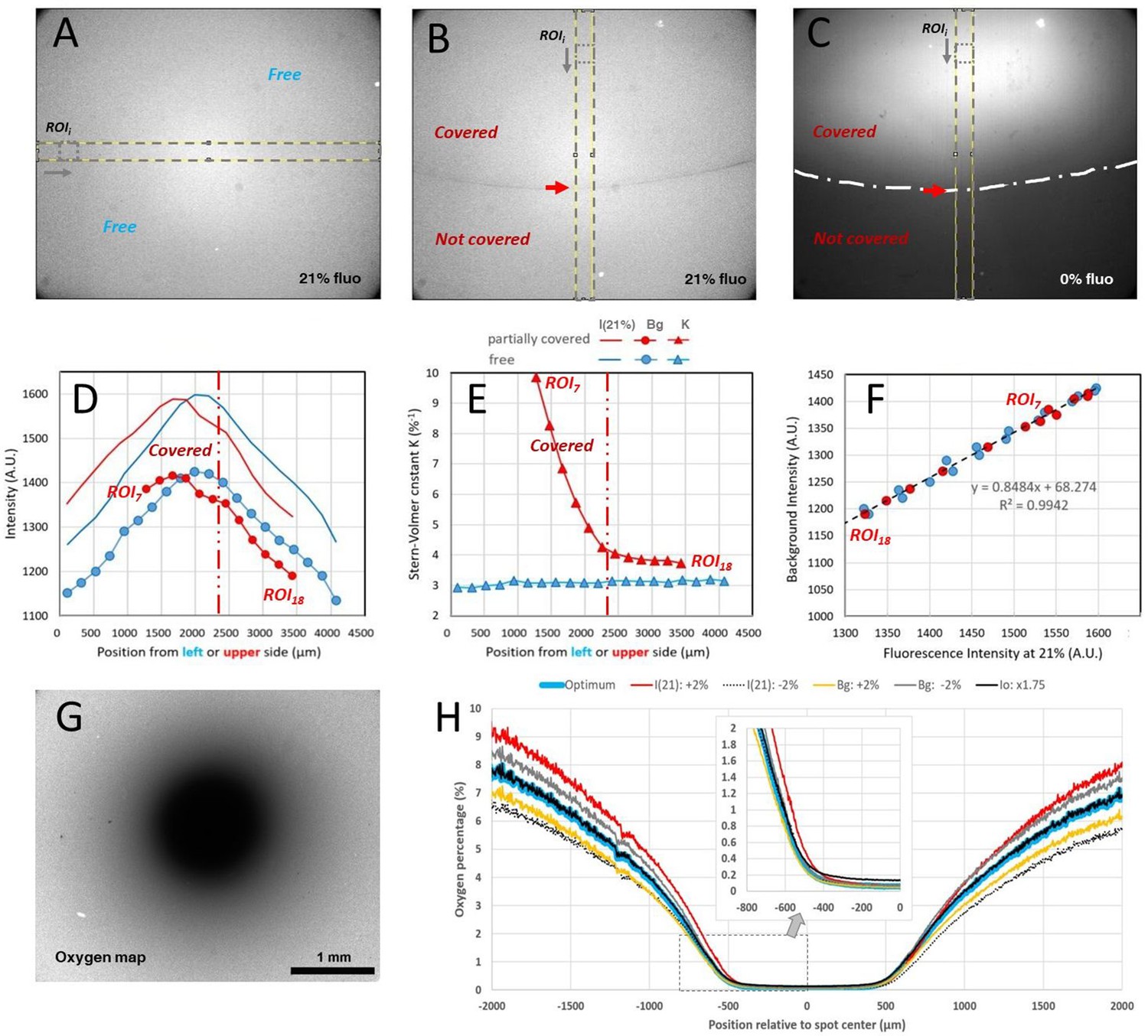
Typical calibration data and oxygen profile measurement with covered sensing films for the spot assay.
(A) Homogeneous 21% O2 level fluorescence image of an uncovered sensing film. (B) Homogeneous 21% O2 level fluorescence image of sensing film partially covered by a plain coverglass simulating the border of the spot assay (the red arrow indicates the glass boundary also depicted as a long dotted line in C. (C) Fluorescence intensity when pure N2 was flushed for 80 min (same region as in B) with the partial coverage of the sensing film). (D) Measured intensity at 21% O2 level (solid line) and fitted background Bg (bullets) for different ROI positions depicted in yellow in A for uncovered film (blue color) and in B for partially covered film (red color). (E) Fitted Bg (bullets) and Stern-Volmer sensitivity parameter K (triangle) along the ROI positions for the uncovered (blue color) and partially covered situation (red color). (F) Fitted Bg plotted as a function of the 21% O2 level intensity for the uncovered and covered situations. (G-H) Calculated O2 map of a Dictyostelium spot covered and corresponding profile along a median horizontal line. Colors correspond to slight changes within the experimental uncertainty of the parameters used for the calculation, insets correspond to the hypoxic (~0–2%) left side of the profile.
-
Figure 2—figure supplement 3—source data 1
Raw data for Figure 2—figure supplement 3.
- https://cdn.elifesciences.org/articles/64731/elife-64731-fig2-figsupp3-data1-v1.xlsx
Figure 2—figure supplement 4
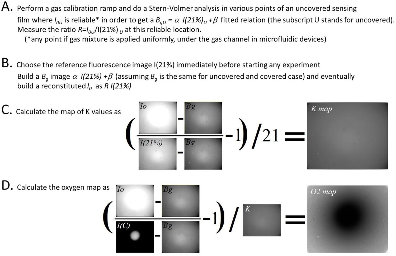
Image analysis pipeline to quantify oxygen map from O2 sensitive sensing films.
Images correspond to an hypoxic circular zone created by a confined Dictyostelium spot.
Figure 2—figure supplement 5
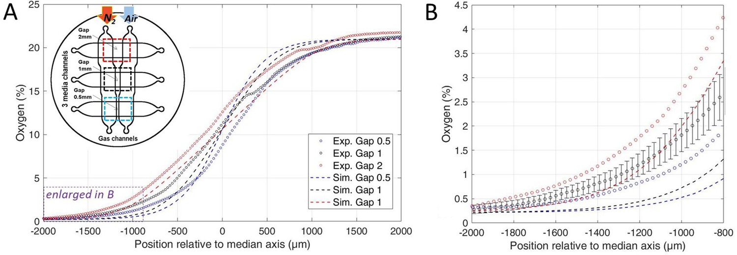
Numerical simulations of oxygen profiles.
(A) Comparison of the measured stationary oxygen profile in the microfluidic device (circles) and simulated ones (dotted lines) for the three gaps. Oxygen is measured thanks to the sensing film. The inset shows the gas injection conditions in the device: pure N2 and air are flushed in left and right gas channel, respectively. (B) Enlarged oxygen profile in the hypoxic side. The estimated error bar on experimental measurements (showed for clarity on gap 1 mm data only) is explained in Materials and methods. Simulations are made with Comsol and explained in Methods.
-
Figure 2—figure supplement 5—source data 1
Raw data for Figure 2—figure supplement 5.
- https://cdn.elifesciences.org/articles/64731/elife-64731-fig2-figsupp5-data1-v1.xlsx
Figure 2—figure supplement 6
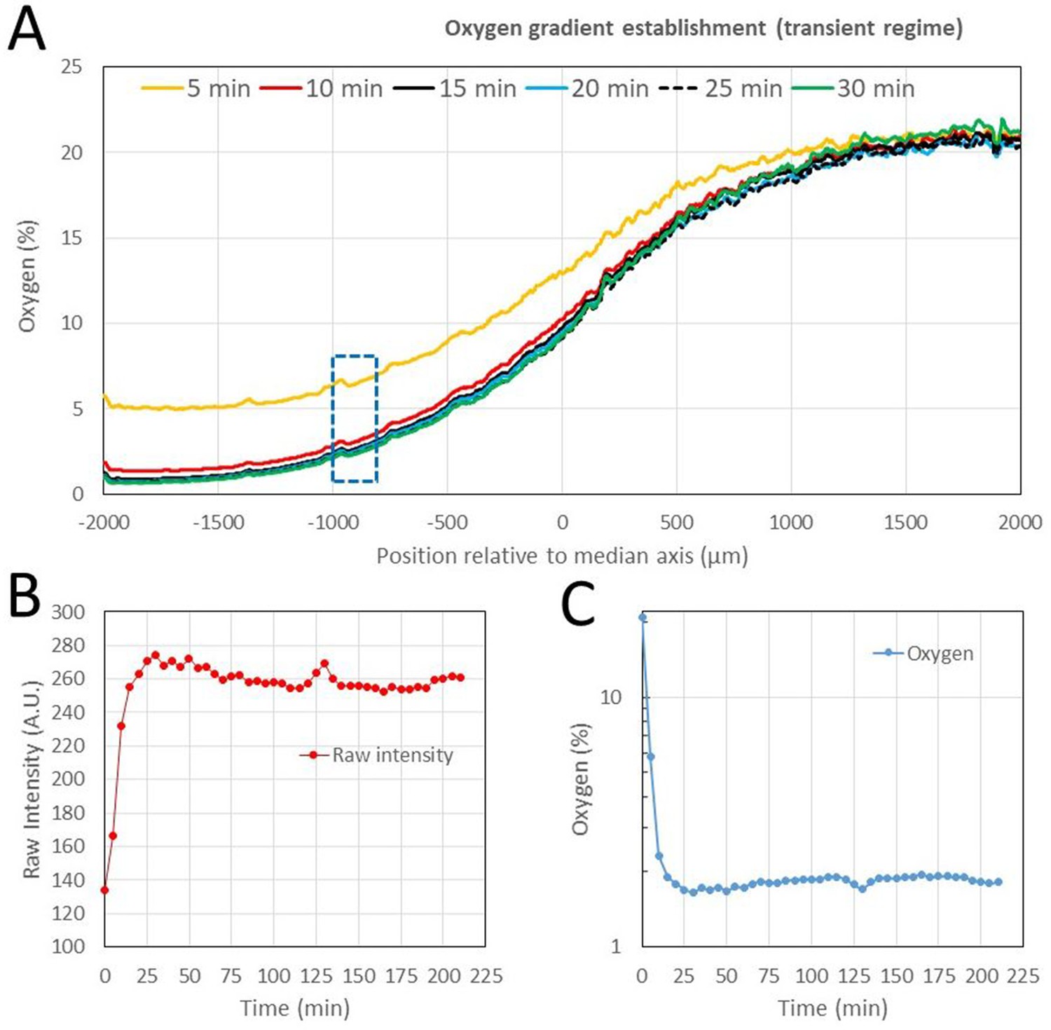
Experimental oxygen gradient establishment in the microfluidic device (gap 0.5 mm).
Pure N2 and air are flushed at time 0 in left and right gas channel, respectively. (A) Oxygen profile measured using the sensing films at 5 min time interval. (B-C) Raw intensity and measured oxygen in the ROI between −1000 µm and −800 µm from the device median axis in the region where the oxygen is about 1.5% (dotted region in A). Within 15 min, each signal reached 95% of its equilibrium value.
-
Figure 2—figure supplement 6—source data 1
Raw data for Figure 2—figure supplement 6.
- https://cdn.elifesciences.org/articles/64731/elife-64731-fig2-figsupp6-data1-v1.xlsx
Figure 2—figure supplement 7
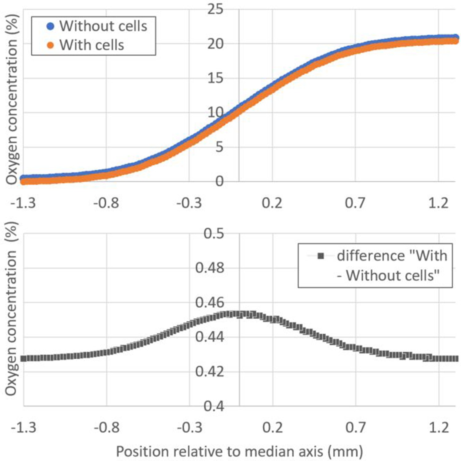
Influence of plated cells on the steady oxygen tension in the microfluidic device (Computational results).
(A) Absolute value of the oxygen concentration as a function of the position relative to the median axis of the device for the gap 1 mm channel in presence (orange markers) or absence of cells (blue markers). Nitrogen is supplied on the left gas channel and 21% O2 is supplied on the right channel. Cells density was taken as 500 cells/mm2, which is the upper experimental limit. (B) Corresponding difference between the two simulated situations (presence and absence of cells). In the region of interest where cells exhibit a strong aerotactic response (i.e., around 1% O2 or −1 mm from the median axis), this difference is around 0.43% O2 which is comparable to the error bar on O2 measurements using sensing films (Figure 2B). The rate of oxygen consumption by Dd cells was taken as 1.2.10−16 mol.cell−1.s−1.
-
Figure 2—figure supplement 7—source data 1
Raw data for Figure 2—figure supplement 7.
- https://cdn.elifesciences.org/articles/64731/elife-64731-fig2-figsupp7-data1-v1.xlsx
Figure 2—figure supplement 8
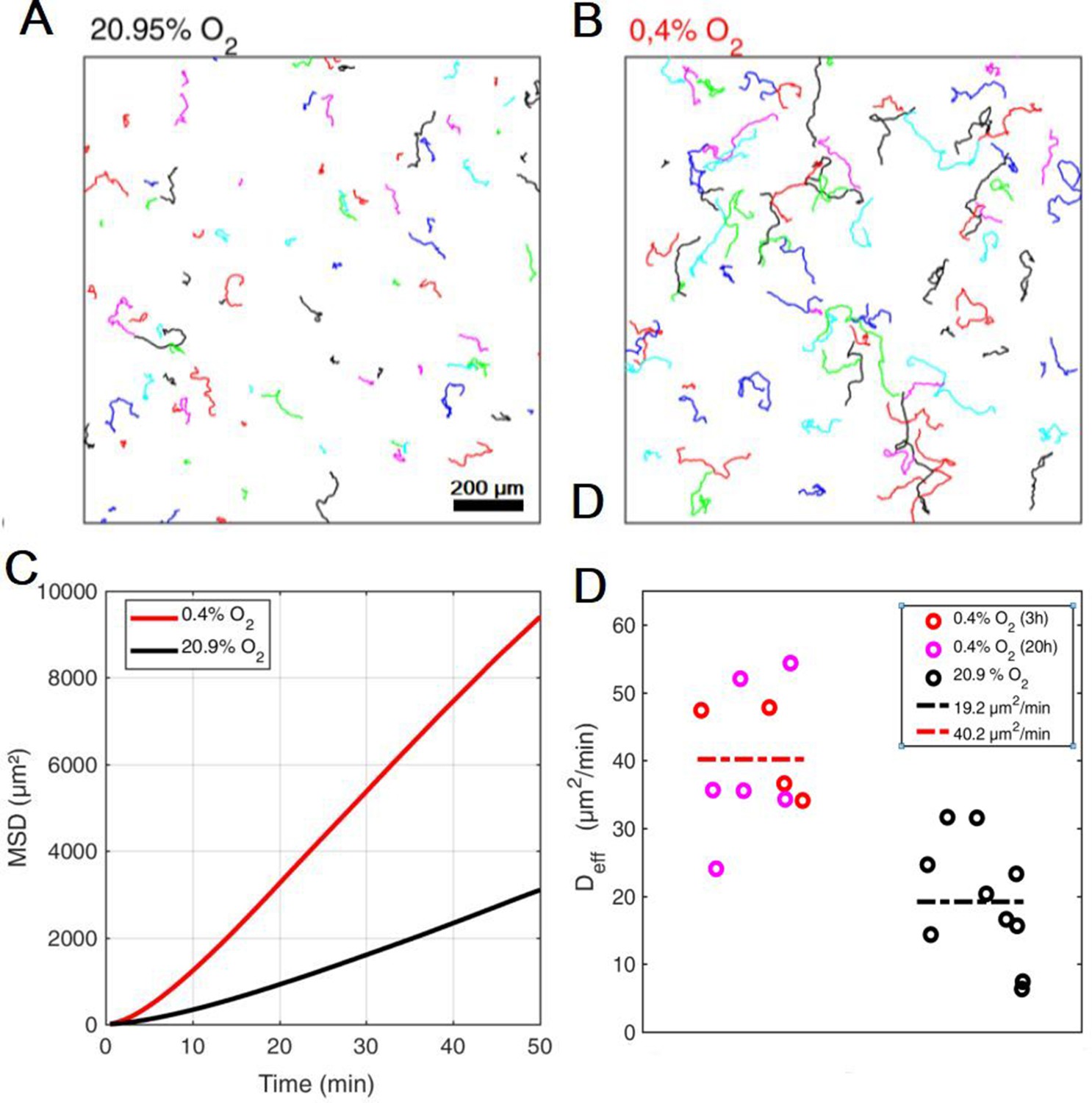
Aerokinesis of Dd cells in homogenous environments.
(A-B) Representative cell trajectories over 1 hr in either atmospheric, C=20.95% (A) or hypoxic, C=0.4% (B) conditions. (C) Quantification of cell motility as mean square displacements in both conditions. (D) Effective diffusion constants in both conditions, also shown after 3 and 20 hr in hypoxic conditions. Dashed lines represent the mean in each conditions over 10 fields of view stemming from five independent experiments in each case.
-
Figure 2—figure supplement 8—source data 1
Raw data for Figure 2—figure supplement 8.
- https://cdn.elifesciences.org/articles/64731/elife-64731-fig2-figsupp8-data1-v1.xlsx
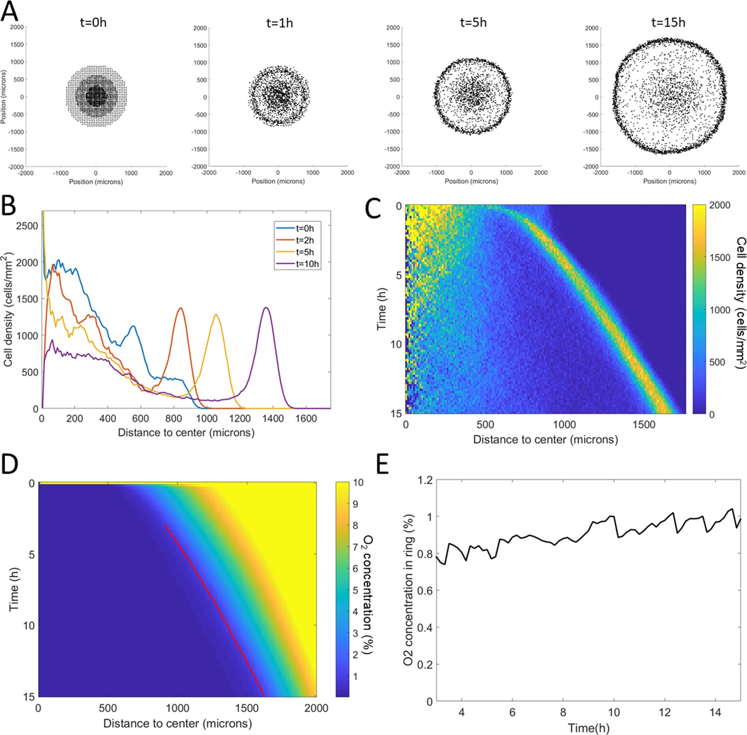
Figure 3
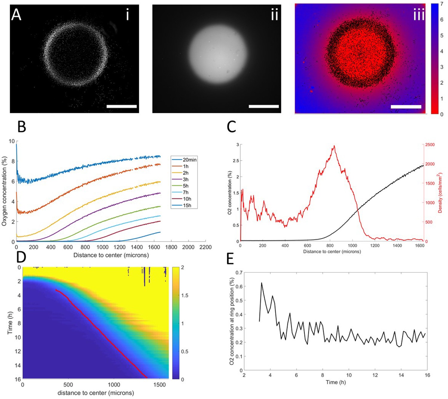
Interplay between ring dynamics and O2 profiles.
(A) (i) Treated image showing cell distribution at t=10h, (ii) raw fluorescent signal indicative of strong O2 depletion, (iii) reconstructed image showing the center of mass of all detected cells and quantitative O2 profiles (colorbar, in % of O2), scale bars: 1 mm. (B) O2 profiles averaged over all angles and shown at different times. (C) Radial profile of cell density and O2 concentration at t=10h showing the position of the ring relative to the O2 profile. (D) Kymograph of O2 concentration (colorbar in %) with the position of the ring represented as a red line. The colormap is limited to the 0–2% range for readability but earlier time points show concentrations higher than the 2% limit. (E) O2 concentration as measured at the position of the ring as a function of time showing that the ring is indeed following a constant concentration after a transitory period.
-
Figure 3—source data 1
Raw data for Figure 3.
- https://cdn.elifesciences.org/articles/64731/elife-64731-fig3-data1-v1.mat
Figure 4 with 3 supplements
Minimal Potts model of ring formation and migration.
(A) Snapshots of a simulated colony of cells showing the formation of highly dense ring of cells. (B) Cell density profiles averaged over all angles for four different times. (C) Corresponding kymograph of cell density (colorbar in cells/mm2) as a function of time and distance to the center. Quantification in terms of microns and hours is described in the Materials and methods section. (D) Kymograph of O2 concentration (colorbar in %) with the position of the ring represented as a red line. The colormap is limited to the 0–10% range for readability but earlier time points show concentrations higher than the 10% limit. (E) O2 concentration at the ring position as a function of time showing that, here too, the ring follows a constant O2 concentration.
-
Figure 4—source data 1
Raw data for Figure 4.
- https://cdn.elifesciences.org/articles/64731/elife-64731-fig4-data1-v1.mat
Figure 4—figure supplement 1
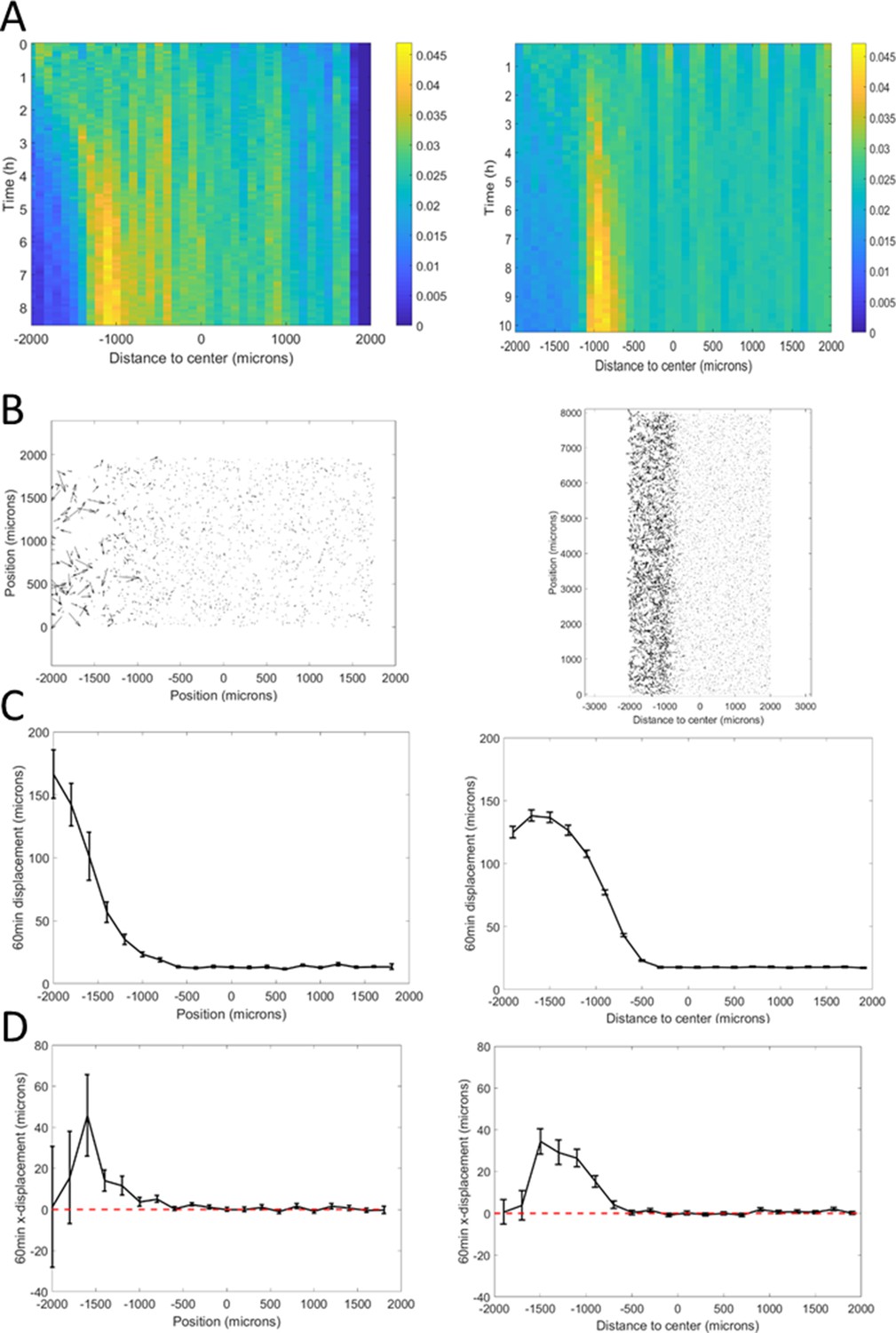
Adjusting Potts model (right) to microfluidic experiments (left).
(A) Density kemographs showing cell accumulation in a low oxygen region. Colorbar represents the fraction of all cells within a bin in distance. (B) Vectorial displacements displayed by cells over 1 hr. Higher activity at low oxygen concentrations, on the left, is clearly visible in both cases. (C) Quantification of cell activity as the norm of the displacements over 1 hr at different positions in the central channel. (D) Quantification of cell bias as the displacement of the cells in the x-direction over 1 hr. In C and (D), each point is the mean ± std of cells within the given distance bin, n=3392 cells total for experiments (left) and n=7520 cells total for simulations (right).
-
Figure 4—figure supplement 1—source data 1
Raw data for Figure 4—figure supplement 1, experiments corresponding to the left column.
- https://cdn.elifesciences.org/articles/64731/elife-64731-fig4-figsupp1-data1-v1.mat
-
Figure 4—figure supplement 1—source data 2
Raw data for Figure 4—figure supplement 1, simulations corresponding to the right column.
- https://cdn.elifesciences.org/articles/64731/elife-64731-fig4-figsupp1-data2-v1.mat
Figure 4—figure supplement 2
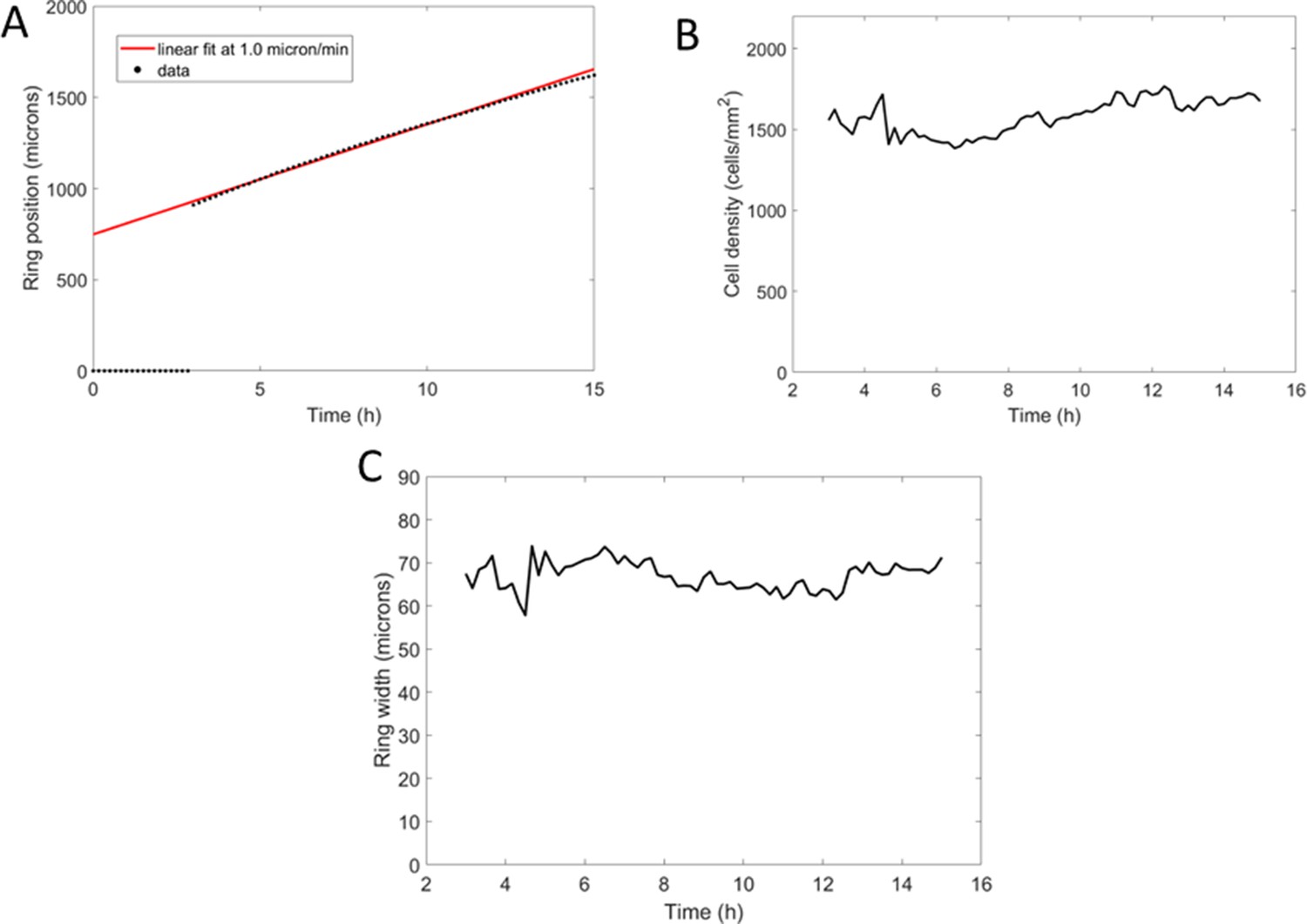
Potts model ring features with parameters adjusted from the microfluidic experiments (Figure 4—figure supplement 1).
(A) Position of the ring as a function of time along with a linear fit yielding a speed of 1.1 µm/min. (B) Cell density within the ring as a function of time, after its formation. (C) Width of the ring as a function of time.
-
Figure 4—figure supplement 2—source data 1
Raw data for Figure 4—figure supplement 2.
- https://cdn.elifesciences.org/articles/64731/elife-64731-fig4-figsupp2-data1-v1.mat
Figure 4—figure supplement 3
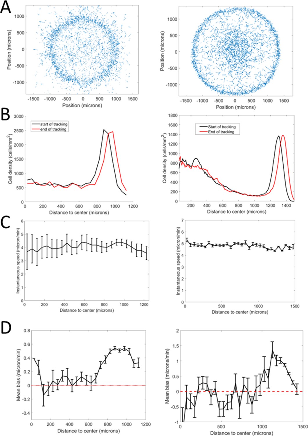
Comparison of cell behavior in spot experiments (left) and Potts models (right).
(A) Sample vectorial displacements over 1 hr. (B) Cell density profiles at the beginning (black) and end (red) of the time window used for cell tracking. This indicates ring position for other plots. (C) Quantification of cell velocities as a function of position. (D) Mean bias in the radial direction measured as the norm of the projected velocity in that direction. In (C) and (D), each point is the mean±std of cells within the given distance bin, n=4715 cells total for experiments (left) and n=5670 cells total for simulations (right).
-
Figure 4—figure supplement 3—source data 1
Raw data for Figure 4—figure supplement 3, experiments corresponding to the left column.
- https://cdn.elifesciences.org/articles/64731/elife-64731-fig4-figsupp3-data1-v1.mat
-
Figure 4—figure supplement 3—source data 2
Raw data for Figure 4—figure supplement 3, simulations corresponding to the right column.
- https://cdn.elifesciences.org/articles/64731/elife-64731-fig4-figsupp3-data2-v1.mat
Figure 5 with 2 supplements
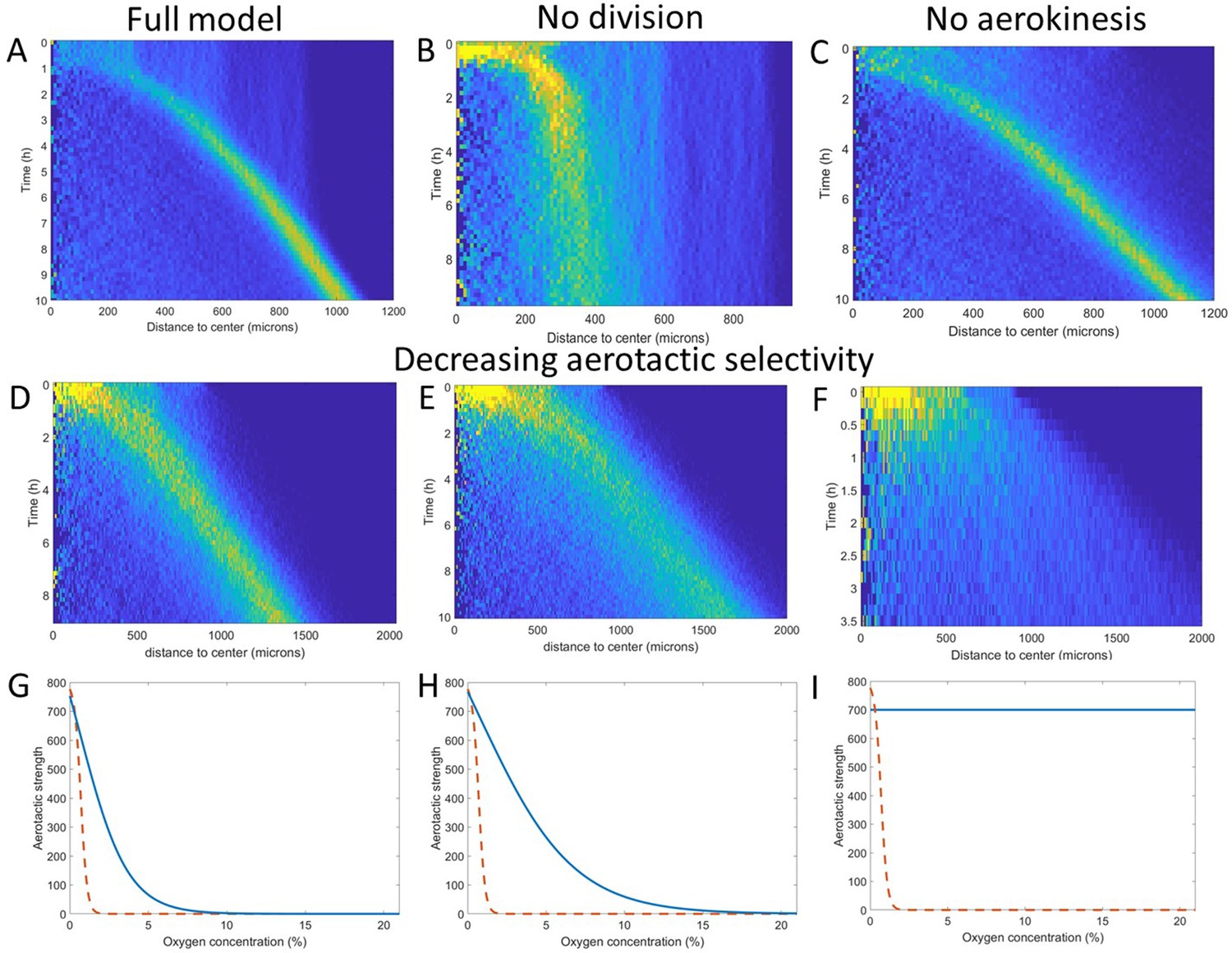
Key ingredients of the Potts model by density kymograph (DK) evaluation.
(A) DK for the full model with reduced oxygen consumption as a basis for comparison. (B) DK in the absence of cell division, note the difference in length scale showing a clear limitation of motion in that case. (C) DK in the absence of aerokinesis (cell activity is not modulated by local oxygen concentrations). (D) DK with a modulation of aerotactic strength as shown in (G), note the wider ring. (E) DK with a modulation of aerotactic strength as shown in (H). (F) DK with a modulation of aerotactic strength as shown in (I), no ring appears and cells quickly migrate outwards as shown by the difference in time scales. (G–I) Three different aerotactic modulations, in blue, compared to the one used in the full model, shown in (A), drawn here as a red dashed line.
-
Figure 5—source data 1
Raw data for Figure 5.
- https://cdn.elifesciences.org/articles/64731/elife-64731-fig5-data1-v1.mat
Figure 5—figure supplement 1
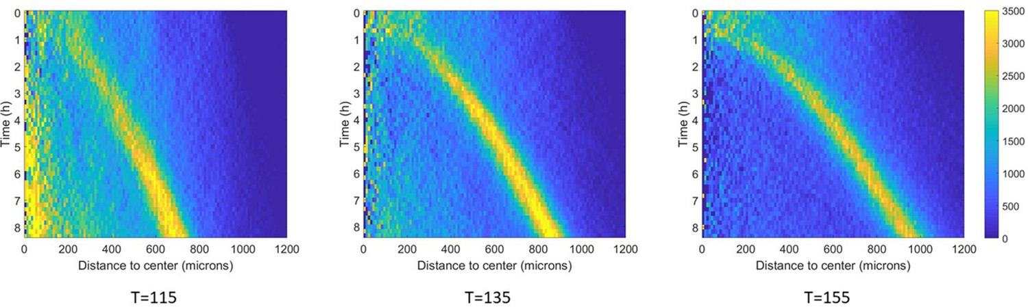
Effect of temperature on ring migration in Potts models.
Density kemographs (all similarly scaled) of the full model, deprived of aerokinesis, at three different temperatures. Colorbar represents cell density in cells/mm2. As temperature increases, fewer cells are left behind the ring and the ring moves at faster velocities.
-
Figure 5—figure supplement 1—source data 1
Raw data for Figure 5—figure supplement 1.
- https://cdn.elifesciences.org/articles/64731/elife-64731-fig5-figsupp1-data1-v1.mat
Figure 5—figure supplement 2
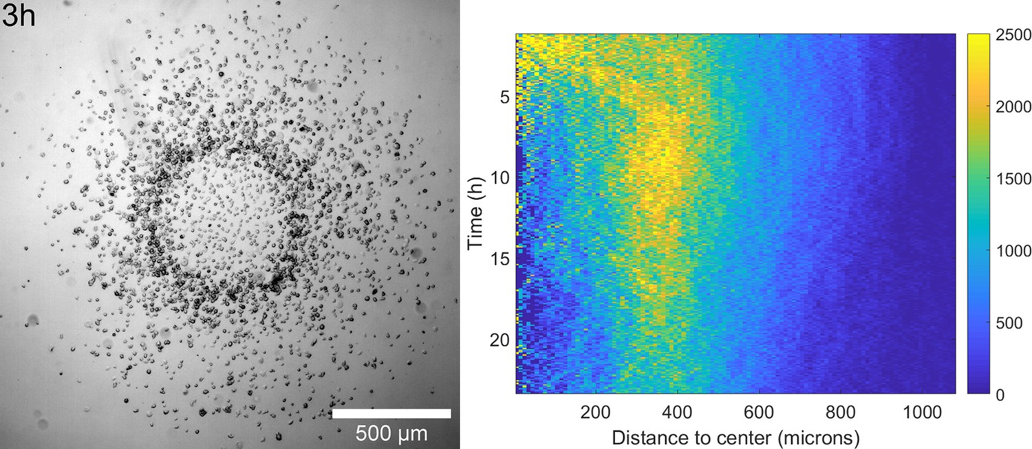
Ring formation in a phosphate buffer.
Left: Snapshot of a spot assay in phosphate buffer at t=3h clearly showing the formation and migration of a dense ring of cells. Right: corresponding density kemograph (cell densities in cells/mm2) showing clear similarities with the predictions of Figure 5B.
-
Figure 5—figure supplement 2—source data 1
Raw data for Figure 5—figure supplement 2.
- https://cdn.elifesciences.org/articles/64731/elife-64731-fig5-figsupp2-data1-v1.mat
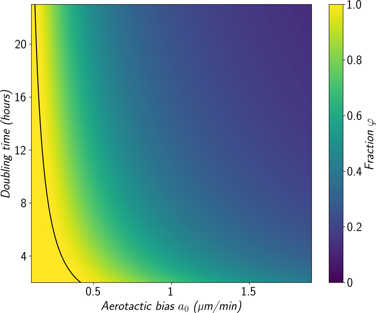
Figure 6 with 1 supplement
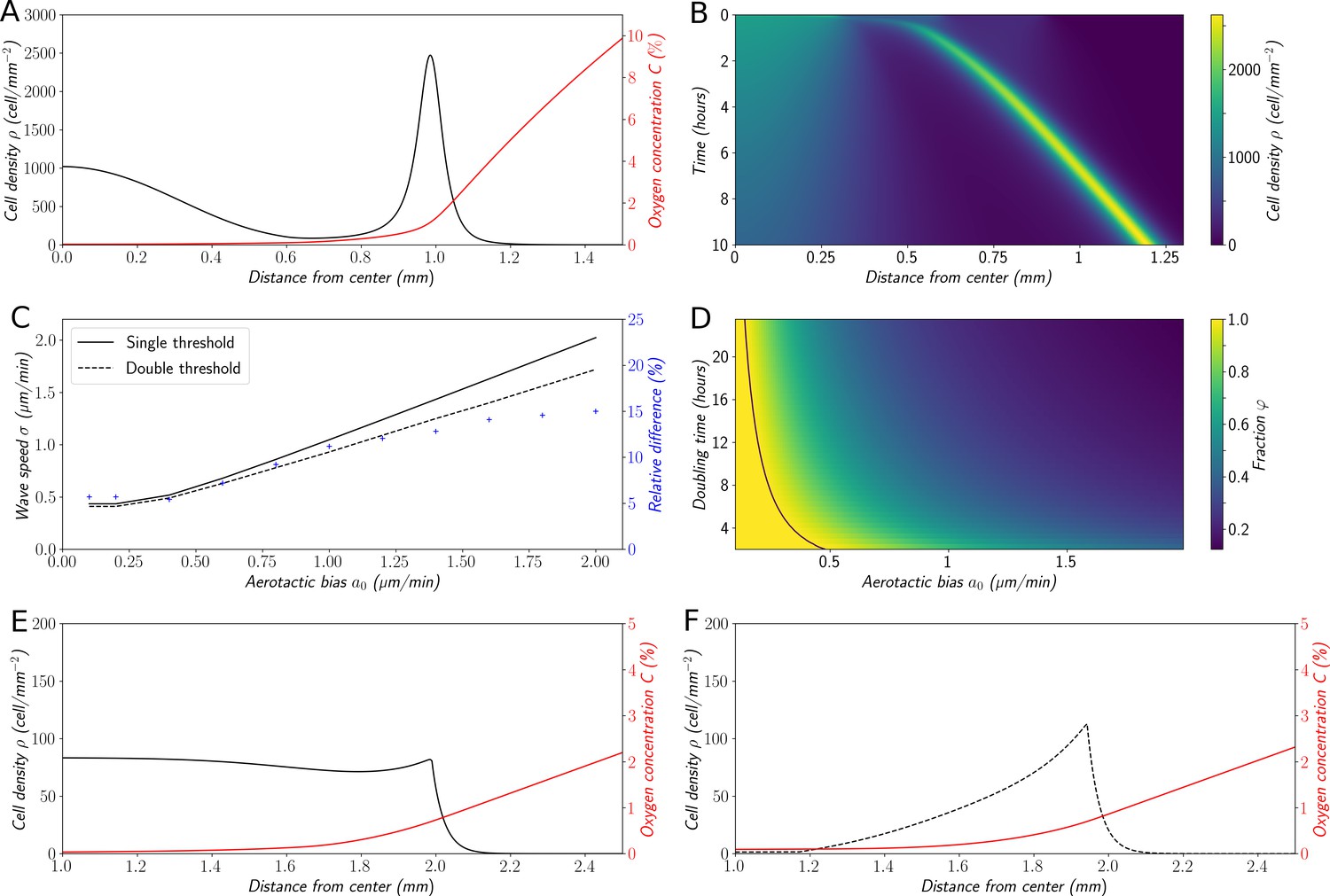
Variations on the ‘Go or Grow’ hypothesis.
(A) Cell density and O2 concentration profiles for the mean-field model (Equations 1 and 2). (B) Corresponding kymograph of cell density (colorbar in cells/mm2) as a function of time and distance to the center. (C) Comparison of wave speeds for the elementary ‘Go or Grow’ model, given by Formula Equation 6, and the ‘Go or Grow’ model with a second threshold, obtained by numerical simulation (solid and dotted lines respectively). The relative difference between the speeds of the two models is represented by crosses. (D) Heatmap of as a measure of the relative contribution of cell division to the overall wave speed in the space parameter and for the ‘Go or Grow’ model (Equation 5), where is given by Formula Equation 6. The curve is depicted in black. (E) Cell density and O2 concentration profiles for the ‘Go or Grow’ model with , and . (F) Cell density and O2 concentration profiles for the ‘Go or Grow’ model with two thresholds: cells undergo aerotaxis with a constant advection speed when the O2 concentration is in the range with , . In both cases, thresholds coincide with the cusps in the profiles.
-
Figure 6—source data 1
Zip file containing raw data for Figure 6 and associated Python code for simulations.
- https://cdn.elifesciences.org/articles/64731/elife-64731-fig6-data1-v1.zip
Figure 6—figure supplement 1
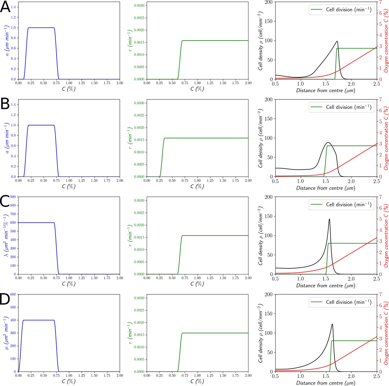
Structural variations of (Equation 1).
(A and B) The left column represents . (C) The left column corresponds to a linear gradient sensing mechanism with . (D) The left column corresponds to a logarithmic gradient sensing mechanism with . For (C and D), the multiplicative factors of and have been chosen such that the speed of the front . The middle column represents the cell division rate . The right column represents the corresponding cell density and O2 concentration profiles. The green curve represents the cell division rate as a function of the position. (A) , (B) , (C) , (D) .
-
Figure 6—figure supplement 1—source data 1
Zip file containing raw data for Figure 6—figure supplement 1 and associated Python code for simulations.
- https://cdn.elifesciences.org/articles/64731/elife-64731-fig6-figsupp1-data1-v1.zip
Figure 7 with 3 supplements
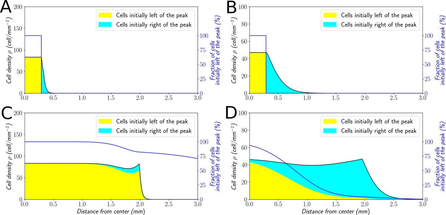
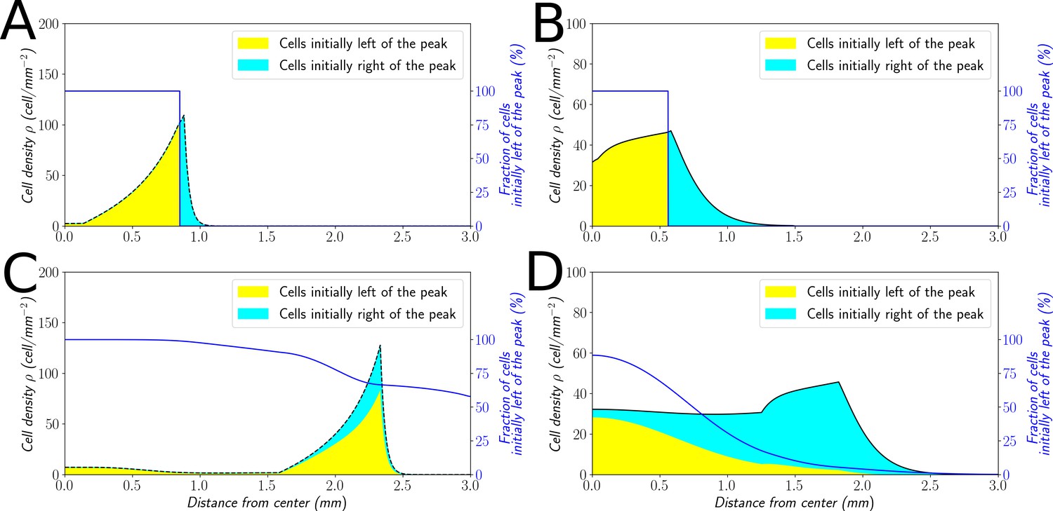
Classification of the expansion type in the ‘Go or Grow’ model.
Cells initially on the left-hand side or right-hand side of the peak get labeled differently (A and B). The labeling is neutral and does not change the dynamics of the cells. We let evolve the two colored population for some time and observe the mixing of the colors (C and D). (A and C) With , the wave is pushed wave and after some time the front undergoes a spatially uniform mixing. (B and D) With , the wave is pulled and only the fraction initially in the front is conserved in the front. and for all conditions.
-
Figure 7—source data 1
Zip file containing raw data for Figure 7 and associated Python code for simulations.
- https://cdn.elifesciences.org/articles/64731/elife-64731-fig7-data1-v1.zip
Figure 7—figure supplement 1
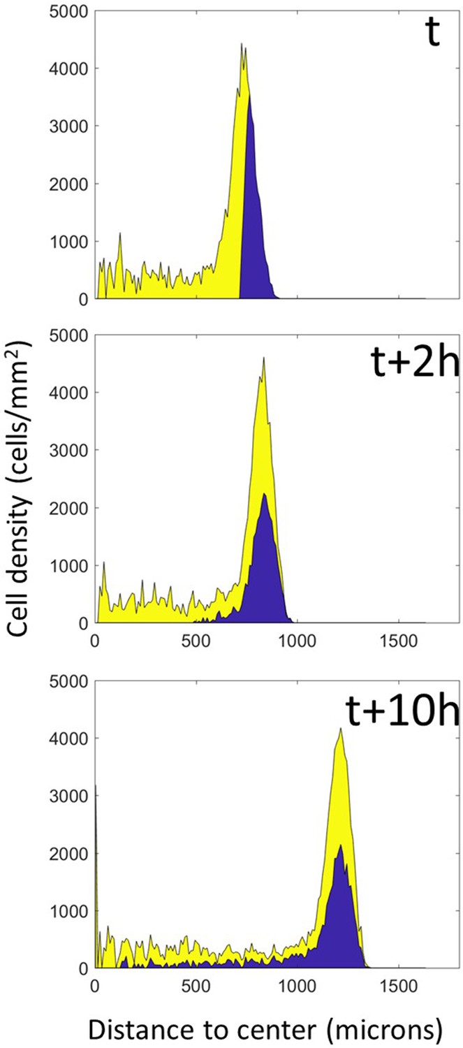
Mixing in Potts models.
A simulation of the full model was stopped at an arbitrary time and cells were colored according to their position at this time. The simulation was then restarted from this time point and left to run for the equivalent of 10 hr, at which point complete mixing of both populations is clearly visible.
-
Figure 7—figure supplement 1—source data 1
Raw data for Figure 7—figure supplement 1.
- https://cdn.elifesciences.org/articles/64731/elife-64731-fig7-figsupp1-data1-v1.mat
Figure 7—figure supplement 2
Heatmap of as a measure of the relative contribution of cell division to the overall wave speed in the space parameter and for the ‘Go or Grow’ model with a second threshold, under the specific condition that O2 consumption term be and that O2 concentration may be negative (see Materials and methods).
The curve is depicted in black.
-
Figure 7—figure supplement 2—source data 1
Zip file containing raw data for Figure 7—figure supplement 2 and associated Python code for simulations.
- https://cdn.elifesciences.org/articles/64731/elife-64731-fig7-figsupp2-data1-v1.zip
Figure 7—figure supplement 3
Classification of the expansion type in the ‘Go or Grow’ model with a second-threshold.
Cells initially on the left-hand side or right-hand side of the peak get labeled differently (A and B). The labeling is neutral and does not change the dynamics of the cells. We let evolve the two colored population for some time and observe the mixing of the colors (C and D). (A and C) With , the wave is pushed and after some time the front undergoes a spatially uniform mixing. (B and D) With , the wave is pulled and only the fraction initially in the front is conserved in the front.
-
Figure 7—figure supplement 3—source data 1
Zip file containing raw data for Figure 7—figure supplement 3 and associated Python code for simulations.
- https://cdn.elifesciences.org/articles/64731/elife-64731-fig7-figsupp3-data1-v1.zip
Videos
Video 1
Initial phase (0–4 hr) of ring formation and migration.
Scale bar: 500 μm.
Video 2
High framerate, high-resolution imaging of cell dynamics in and behind the ring over 15 min.
Time is in min:s and the scale bar represents 100 μm.
Video 3
Reconstruction of cell and oxygen dynamics from a spot experiment on an oxygen sensor.
Cell positions are shown as black dots, oxygen in colors (scale bar in %). The entire movie spans 15 hr of experiment.
Video 4
Dynamics of the Potts model reproducing microfluidic experiments.
Low oxygen regions are on the left and high oxygen on the right. Cell positions are shown as black dots and the entire movie represents the equivalent of 10 hr of experiments.
Video 5
Dynamics of the Potts model reproducing the spot experiments.
Cell positions are shown as black dots and the oxygen is in colors (in %).
Video 6
Spot assay in phosphate buffer.
Left: cell dynamics show the formation and migration of a ring of cells up to 4 hr at which point it started disintegrating and aggregates started forming around 10 hr. Right: polar visualization of cell dynamics with angles shown vertically and distance to the center horizontally. This visualization clearly shows the early propagation of a ring of cells.
Video 7
Ring fusion during experiments (top) and as predicted by the Potts model (bottom).
Note that this Potts model is a non-quantitative version and, as a result, space and time are in arbitrary units and thus not shown.
Video 8
3D Potts simulations.
Top : with oxygen sources on all sides. Bottom: with oxygen sources on all sides except on the bottom. The left column shows the behavior of the whole cell assembly in 3D (original cells are in blue, cells created during the process are shown in green). The middle column is an xz slice of the cell behavior to show that the 3d structures are indeed spheres or pseudo-spheres. The right column is the same slice as in the middle but showing oxygen profiles as a colormap.
Additional files
-
Source data 1
Detailed measurements for quantities presented in the text as means ± standard deviations.
- https://cdn.elifesciences.org/articles/64731/elife-64731-data1-v1.xlsx
-
Transparent reporting form
- https://cdn.elifesciences.org/articles/64731/elife-64731-transrepform-v1.docx
Download links
A two-part list of links to download the article, or parts of the article, in various formats.
Downloads (link to download the article as PDF)
Open citations (links to open the citations from this article in various online reference manager services)
Cite this article (links to download the citations from this article in formats compatible with various reference manager tools)
Hypoxia triggers collective aerotactic migration in Dictyostelium discoideum
eLife 10:e64731.
https://doi.org/10.7554/eLife.64731


