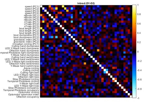
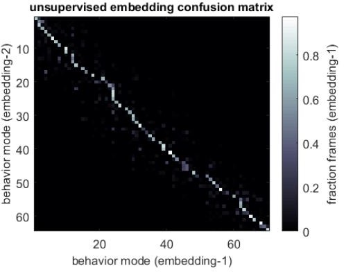
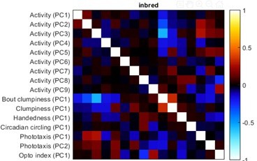
The structure of behavioral variation within a genotype
Figures
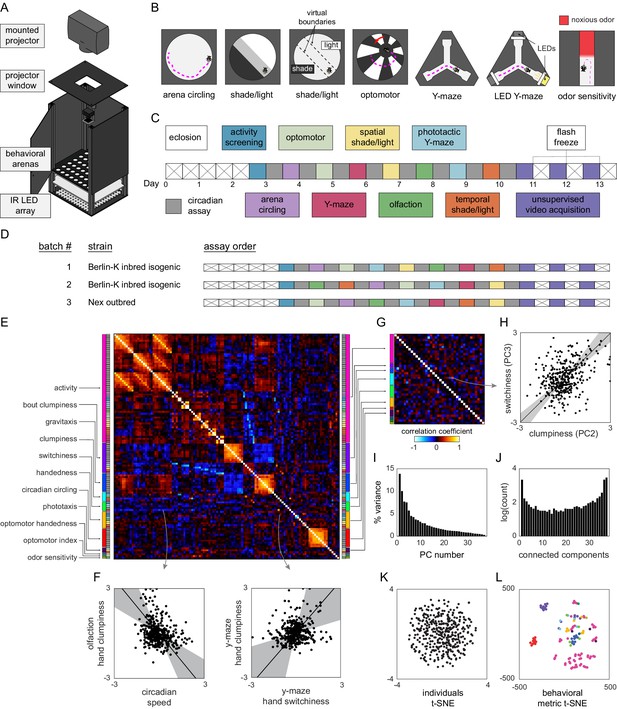
Decathlon experimental design and structure of intragenotypic behavioral variation.
(A) Schematic of the imaging rig used for most Decathlon experiments. (B) Schematics of the behavioral assays, illustrating the geometry of the arenas and stimulus structure. (C) Timeline of the Decathlon experiment. Colors indicate the assays conducted on each day, half-black half-white blocks indicate the circadian assay and storage in 96-well plates. (D) Timelines of the three Decathlon experiments, indicating the randomized order of assays 2–8. (E) Full correlation matrix of all raw behavioral measures taken in the Decathlon. Colored blocks indicate blocks of measures we thought a priori might be correlated (outer blocks, text labels). Inner blocks indicate assay. (F) Example scatter plots associated with measure correlations. Points are individual flies. Line is the best fit (principal component [PC]1 of these points), gray region is the 95% confidence interval of the fit, as determined by bootstrap resampling. (G) Distilled correlation matrix in which all correlated measures represent unexpected relationships. Meaningful correlations in this matrix can be found outside the within-a-priori-group on-diagonal blocks. (H) Example scatter plot from the distilled correlations. Plot elements as in (F). (I) Scree plot of the ranked, normalized eigenvalues, that is, the % variance explained by each PC, of the distilled behavior matrix, versus PC #. (J) Connected components spectrum (see text and Figure 1—figure supplement 10) for the distilled correlation matrix. Height of bars indicates organization at that dimensionality. (K) Points corresponding to individual flies nonlinearly embedded using t-SNE from the 121-dimensional full matrix to two dimensions. (L) Points corresponding to behavioral measures nonlinearly embedded using t-SNE from the 384-dimensional space of flies to two dimensions. Colors indicate groups of measures we expected a priori to be related.
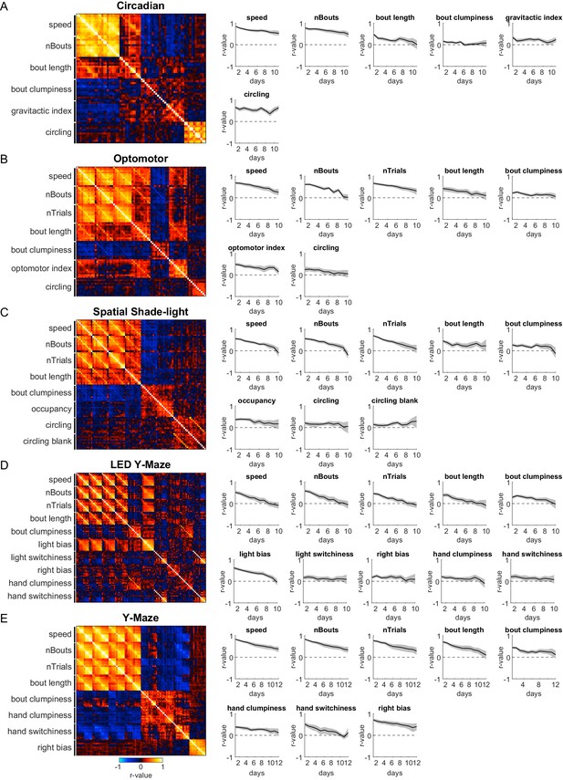
Persistence of primary behavioral measures across assays.
(A) Correlation matrix (left) for 10 retests of the same individuals on a single assay (circadian) across consecutive days. Rows and columns correspond to one of six behavioral measures acquired in this assay and were sorted to cluster the same measures across days. Plots (right) of the correlation coefficient (r) between behavioral measures acquired on day 1 and the day indicated on the x-axis. Shaded gray regions indicate the 95% confidence intervals estimated via bootstrap resampling. Dashed black line denotes no correlation (r = 0). (B–E) Correlation matrices (left) and correlation coefficient plots (right) for the optomotor, Spatial shade-light, LED Y-maze, and Y-maze assays in the style of (A).
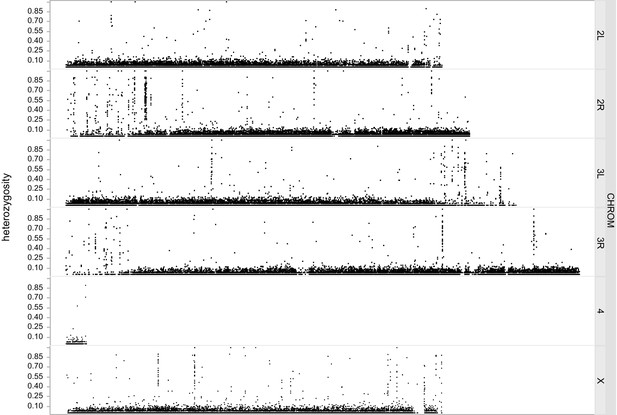
Genomic sequencing to confirm isogeny of Berlin-Kiso.
Fraction of Berlin-Kiso flies (n = 48) that were heterozygous at any given position in the genome. Typically no more than 10% of flies appeared to be variant at a given locus. There was evidence of residual heterozygosity at approximately 75 sites throughout the genome. These can be seen as distinct regions appearing as ‘columns’ of heterozygous sites and are mostly found at the ends of chromosome arms.
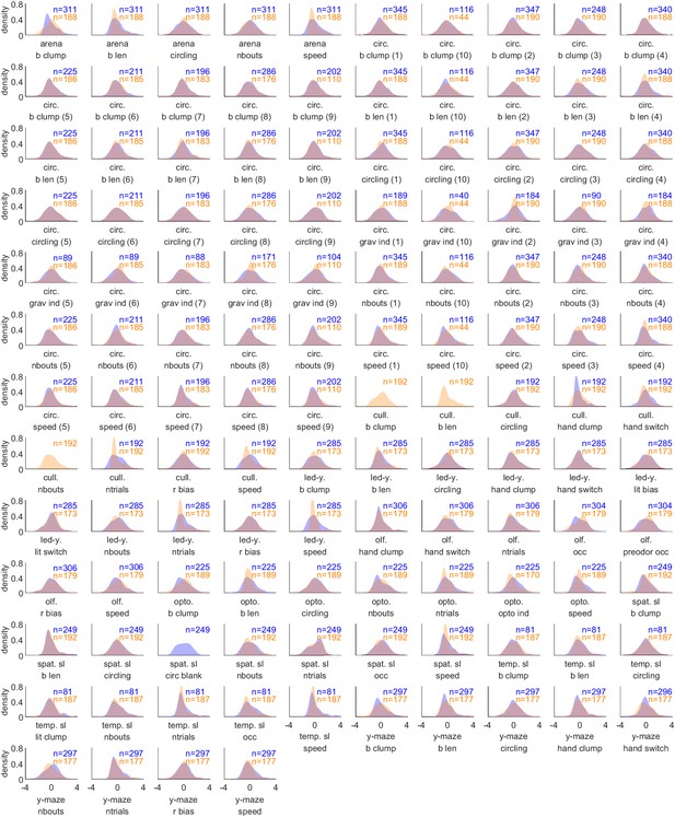
Decathlon behavioral measure distributions.
Kernel density estimates of all z-scored behavioral measures. Density estimates were computed on behavior data after combining both inbred Decathlon iterations and before infilling of missing data. Sample sizes of inbred (blue) and outbred (orange) flies are indicated in the upper-right corners of each plot.
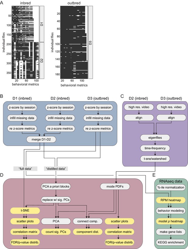
Schematic of the Decathlon analysis pipeline.
(A) Data matrices from the inbred and outbred Decathlon experiments. Rows are flies, columns are behavioral measures. White cells indicate missing data prior to infilling. (B) Decathlon assay behavioral data preprocessing pipeline. Measures are z-scored by imaging session to adjust for batch effects. Missing data is infilled with an alternating least squares (ALS) imputed matrix calculated as the median of 200 ALS imputations. Inbred Decathlon batches D1 and D2 merged into a single behavioral data matrix before analyzing inbred and outbred flies separately. (C) Data acquisition and analysis for the unsupervised behavioral classification pipeline. High-resolution, high-frame rate single-fly videos are aligned to a template fly. Data from D2 (inbred) and D3 (outbred) flies were combined before being compressed into principal component (PC) time series (i.e., eigenflies). PC time series are then decomposed into 25 frequency spectral time series via Morlet wavelet transformation. The resulting high-dimensional data is then embedded into two dimensions with t-SNE and then clustered into discrete behavioral modes via watershed transformation. Data from the Decathlon assays and unsupervised behavioral classifications are analyzed separately. (D) Downstream analyses. Distilled matrices are generated by retaining the significant PCs within each a priori group (see Materials and methods). Distilled, full and, unsupervised data sets are subject to a number of common analyses including PCA, t-SNE embedding, and connected components spectral analysis. (E). Individual flies undergo gene expression profiling via RNAseq. Behavioral metrics are modeled independently by gene expression. Gene lists are then constructed for each behavior by thresholding model significance. Lists are then used as input for KEGG pathway enrichment analysis.
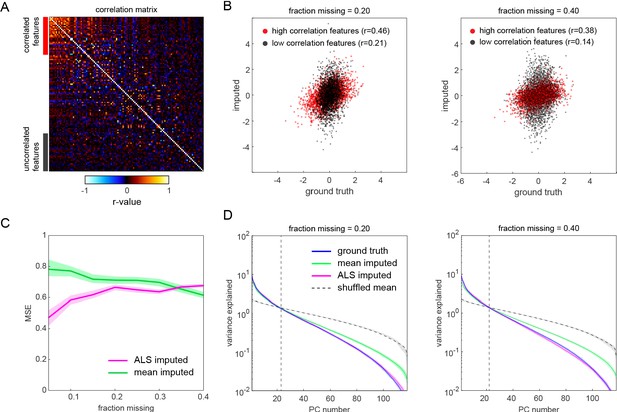
Simulated comparison of matrix-infilling methods.
(A) Correlation matrix of a simulated behavioral measure data set generated from a multivariate normal distribution with a covariance matrix equal to that of the inbred Decathlon behavior measures. We focused on the infilling performance for correlated features (red) and uncorrelated features (gray) in particular. These were defined as behavioral measures with mean correlation coefficient magnitudes in the 75th and 25th percentiles, respectively. (B) Scatter plots of data ground truth vs. infilled values (determined as the median alternating least squares [ALS] imputation over 200 repetitions) after randomly deleting either 20% (left) and 40% (right) of the data. Color indicates whether the data belonged to high or low correlation features as in (A). (C) Comparison of mean squared error (MSE) for mean infilled and ALS average infilled data. (D) Log scree plots of the variance explained for ranked principal components resulting from principal component analysis (PCA) on the ground truth, mean infilled, average ALS infilled, and shuffled matrix.

Correlation of correlation matrix values between inbred-1 vs. inbred-2 and shuffled matrices.
(A) Distributions of correlation of full matrix correlation values across bootstrap replicates. Bootstrapping was performed on individual flies in the data matrices of inbred-1 and inbred-2. (B) As in (A), but for the distilled correlation matrix.
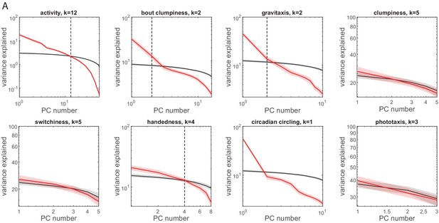
Principal component analysis (PCA) of a priori groups.
(A) Log scree plots of the normalized ranked eigenvalues (i.e., variance explained) for PCA performed on measures from each a priori group separately. Color indicates observed (red) or shuffled (black) data. Shaded regions correspond to 95% confidence intervals as calculated by bootstrap resampling. The number of significant principal components (PCs) (k) was calculated as the highest rank PC above or within the 95% confidence interval of the shuffled matrix variance explained.
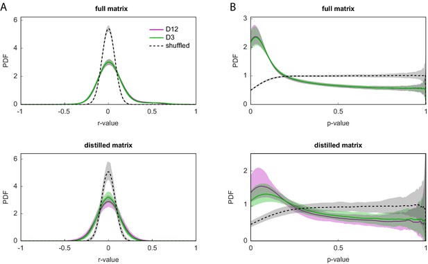
Distribution of correlation coefficients and p-values in the full and distilled correlation matrix.
(A) Kernel density estimates of the unique (i.e., lower matrix triangle) correlation coefficients in the full (top) and distilled (bottom) correlation matrices. Distributions exclude duplicate pairwise and self-correlations. (B) Kernel density of the unique p-values for the correlation coefficients in (A). In all plots, dashed lines indicate distributions for column-wise (i.e., within each feature) shuffled matrices. Shaded regions correspond to 95% confidence intervals calculated by bootstrap resampling.
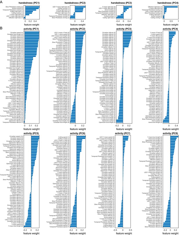
Measure loadings for the handedness and activity a priori groups.
(A) Measure loadings of significant principal components (PCs) for the handedness a priori group. (B) Measure loadings of significant PCs for the activity a priori group. Continues in Figure 1—figure supplement 10.
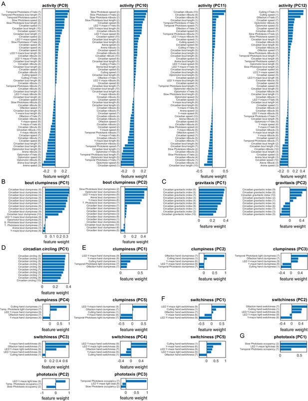
Measure loadings for various a priori groups.
(A) Measure loadings of significant high-rank principal components (PCs) for the activity a priori group. Continues from Figure 1—figure supplement 9. (B–G) Measure loadings of significant PCs for the following a priori groups, respectively: clumpiness, gravitaxis, circadian circling, clumpiness, switchiness, and phototaxis.
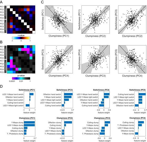
Correlations among the principal components (PCs) of switchiness and clumpiness.
(A) Subset of the distilled correlation matrix corresponding to the significant PCs of switchiness and clumpiness. (B) p-Value matrix for the correlation coefficients in (A). (C) Scatter plots of significant correlations between switchiness and clumpiness. Points correspond to individual flies. Line indicates the line of best fit, and the shaded region indicates the 95% confidence interval of the fit as calculated by bootstrap resampling. (D) Measure loadings for the PCs in (C).
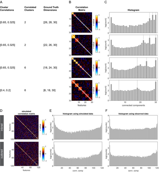
Connected components spectra for determining dimensional organization: simulated data examples.
(A) Parameters used to generate a 200 × 30 ground truth matrix from a multivariate normal distribution. ‘Cluster correlation’ refers to the correlation between features belonging to the same cluster. ‘Correlated clusters’ indicate the total number of such clusters in the matrix. ‘Ground truth dimensions’ indicate the expected peaks in the connected components spectrum. Peak locations correspond in order to (1) the number of high correlation clusters plus the remaining features, (2) the number of high and low correlated clusters plus the remaining features, and (3) the total number of features. (B) Correlation matrices of ground truth data sets generated by sampling 392 values from a multivariate normal distribution with the covariance structure described in (A). Features along the diagonal reflect the constructed correlation clusters. (C) Connected components spectra of the correlation matrices in (B), indicating the ground truth dimensionalities in which the data are organized (dashed lines). Histograms were generated by sweeping 100 thresholds spaced evenly from –1 to 1, applying that threshold to the absolute value of the correlation matrix, treating it as an adjacency matrix, and determining the number of connected components. Peaks at a particular number of connected components indicate that the correlation matrix has that many connected components for a large number of threshold values. (D) Simulated correlation matrices modeled from the observed inbred (top) and outbred (bottom) Decathlon assay behavioral measures. Simulated matrices were generated by sampling from the observed distribution of correlation coefficients after subtracting off the distribution of correlation coefficients from measure-wise shuffled controls. (E, F) Connected components spectra of the modeled (E) or observed (F) correlation matrices for inbred (top) and outbred (bottom) flies.
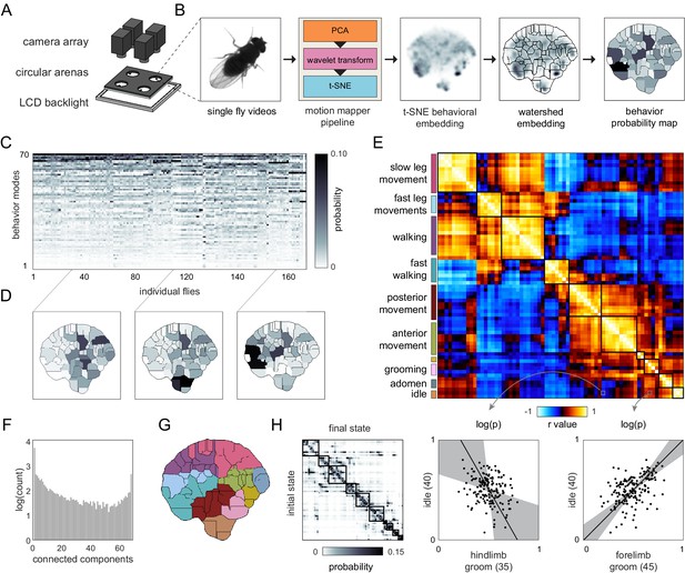
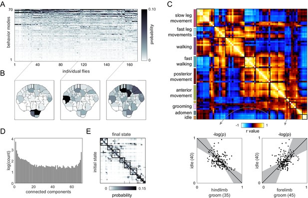
Correlation structure of unsupervised behavioral classifications.
(A) Schematic of the four camera imaging rig used to acquire single fly videos. (B) Overview of the data processing pipeline from single fly videos to behavioral probability maps. (C) Sample individual behavior mode probability density functions (PDFs visualized in an embedded t-SNE space). Discrete regions correspond to watersheds of the t-SNE embedding. (D) Sample individual PDFs mapped to locations in t-SNE space. Discrete regions correspond to watersheds of the t-SNE embedded probability densities. (E) Correlation matrix (top) for individual PDFs with rows and columns hierarchically clustered. Colored blocks indicate labels applied to classifications post hoc. Example scatter plots (bottom) of individual behavioral probabilities. Points correspond to probabilities for individual flies. Line is the best fit (principal component [PC]1 of these points), gray region is the 95% confidence interval of the fit, as determined by bootstrap resampling. (F) Connected components histogram of the thresholded PDF correlation matrix (see Materials and methods). (G) Discrete behavioral map with individuals zones colored by post hoc labels as in (E). (H) Transition probability matrix for behavioral classifications. Entries in the ith row and jth column correspond to the probability of transitioning from state i to state j over consecutive frames. Blocks on the diagonal indicate clusters of post hoc labels as in (E) and (G).
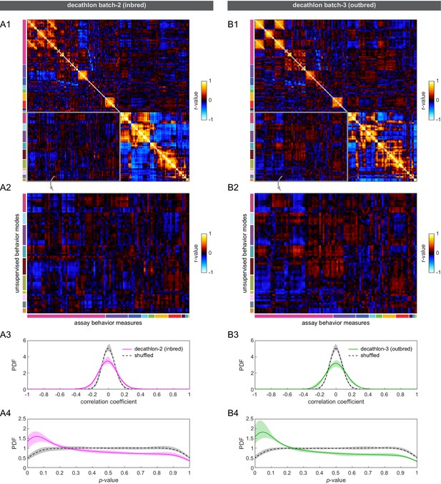
Correlation of Decathlon assay and unsupervised behavioral measures.
(A1–B1) Combined correlation matrices of assay (upper left) and unsupervised (bottom right) behavioral measures for inbred (A) and outbred (B) flies. (A2–B2) Subset of the combined correlation matrix corresponding to pairwise combinations of assay and unsupervised behavioral measures. Colored bars indicate assay a priori groups (columns) and unsupervised behavior manual groupings (rows). (A3–B3) Kernel density estimates of the distribution of pairwise correlation coefficients between assay and unsupervised behavioral measures (solid lines) and shuffled (dashed lines) controls. (A4–B4) Kernel density estimates of the distribution of p-values of the correlation coefficients in (A3–B3). Shaded regions in all panels are 95% confidence intervals determined by bootstrap resampling.
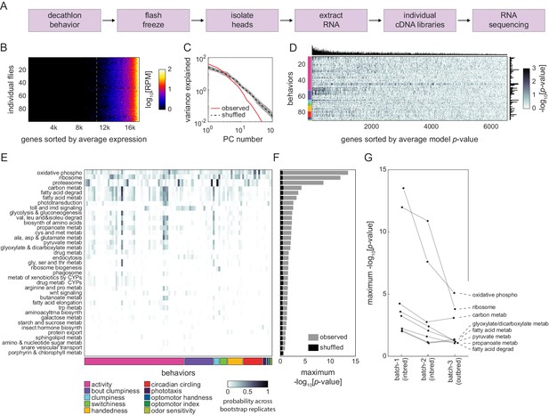
Correlation between individual transcriptomes and behavioral biases.
(A) Steps for collecting transcriptomes from flies that have completed the Decathlon. (B) Data matrix of individual head transcriptomes. Rows are individual flies (n = 98). Columns are 17,470 genes sorted by their mean expression across individuals. The dashed line indicates the mean expression cutoff at 10 reads per million (RPM), below which genes were excluded from analysis. (C) Scree plots of the logged % variance explained for ranked principal components of gene expression variation, for observed (red) and shuffled (black) data. Shaded region corresponds to 95% CI as calculated by bootstrap resampling. (D) Performance heatmap (-log p) of linear models predicting the behavior of individual flies from single-gene expression. Colored bars (left) indicate a priori group identity of behavioral measures (rows). Bar graphs show the number of significant (p<0.05) models for each gene (top) and behavior (right). (E) Heatmap showing the probability across bootstrap replicates of a KEGG pathway being significantly enriched in the list of predictive genes for a given behavior. (F) Bar plot showing the average across bootstrap replicates of the maximum (across behaviors) negative log adjusted p-value of all enriched KEGG pathways. Color indicates results from observed (gray) or shuffled control (black) data. (G) Average maximum adjusted -log p-value for enriched KEGG pathways common to all Decathlon iterations. Pathway labels (right) are ordered by batch 3 (outbred) -log adjusted p-value.
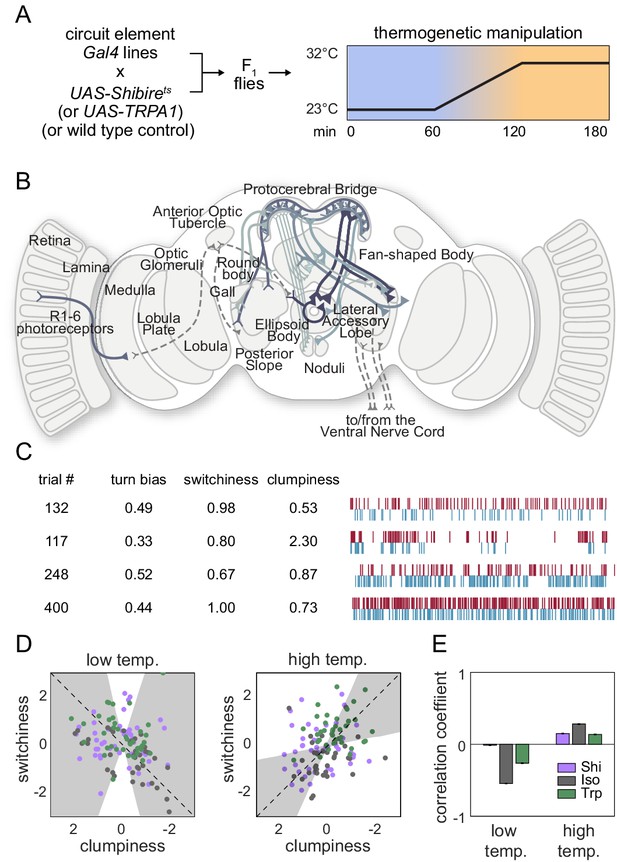
Effect of thermogenetic neural perturbation on clumpiness and switchiness.
(A) Schematic of the experiment for testing the effects of neural perturbation on switchiness and clumpiness. Plot depicts the schema used to activate or silence neurons. (B) Diagram of the various neurons (solid lines) targeted by lines tested in the screen. See Supplementary file 3 for list. (C) Example turn data from individuals exhibiting low and high clumpiness (upper rows) and low and high switchiness (bottom rows). (D) Scatter plots of line average clumpiness and switchiness at the permissive (left) and restrictive (right) temperatures. Lines indicate the line of best fit and shaded regions indicate the 95% confidence of the fit as determined by bootstrap resampling. (E) Average correlation coefficients for each effector type at the permissive and restrictive temperatures. Error bars indicate the 95% confidence interval as determined by bootstrap resampling. Panels (A) and (B) have been reproduced from Figure 2B and G of Skutt-Kakaria et al., 2019 Bioxiv, published under a CC BY 4.0 license.

Structure of behavioral variation in outbred flies.
(A) Distilled correlation matrix for outbred NEX flies. Colored blocks indicate a priori groups as described in Figure 1. (B) Points corresponding to individual flies nonlinearly embedded using t-SNE from the 121-dimensional full matrix to two dimensions. Color indicates whether the flies were inbred (blue) or outbred (orange). (C) Points corresponding to behavioral measures nonlinearly embedded using t-SNE from the 192-dimensional space of flies to two dimensions. Colors correspond to a priori group. (D) Scree plot of the ranked, normalized eigenvalues, that is, the % variance explained by each principal component (PC), of the distilled covariance matrix, versus PC #. (E) Connected components spectra for outbred and inbred correlation matrices (see Materials and methods). (F) Scatter plot of the distilled matrix correlation coefficients for inbred and outbred flies. Points correspond to distilled matrix measure pairs. (G) Example scatter plots of distilled matrix measure pairs for inbred (left) and outbred (right) flies. The rows of plots highlight a pair of measures with qualitatively different (top) and similar (bottom) correlations in inbred and outbred flies.
Correlation structure of outbred unsupervised behavior classifications.
(A) Behavioral classification probability density function (PDF) matrix. Columns correspond to behavioral PDFs for individual outbred flies. (B) Sample individual behavior mode PDFs visualized in an embedded t-SNE space. Discrete regions correspond to watersheds of the t-SNE embedding. (C) Correlation matrix (top) for individual PDFs with rows and columns hierarchically clustered as in Figure 2E. Colored blocks indicate manual labels applied to classifications post hoc as in Figure 2G. Example scatter plots (bottom) of individual behavioral probabilities. Points correspond to probabilities for individual flies. Line is the best fit (principal component [PC]1 of these points), gray region is the 95% confidence interval of the fit, as determined by bootstrap resampling. (D) Connected components histogram of the outbred correlation matrix (see text and Materials and methods). (E) Transition probability matrix for behavioral classifications. Entries in the ith row and jth column correspond to the probability of transitioning from state i to state j. Blocks on the diagonal indicate clusters of post hoc labels as in (C).
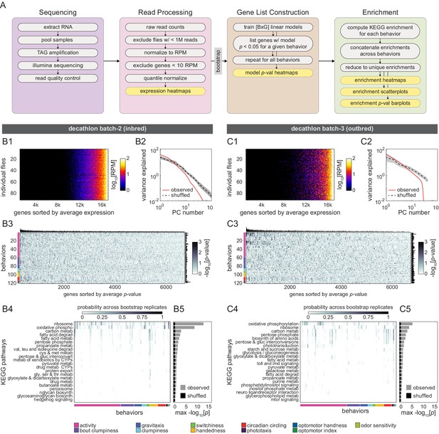
Correlation between individual transcriptomes and behavioral biases.
(A) Schematic of the RNAseq analysis pipeline for both experimental batches. Following sequencing, raw read counts were filtered and quantile normalized. Linear models were fit using individual expression of single genes (G) to predict individual behavioral scores (B) (BxG models total). Gene lists were constructed for each behavior separately from its set of significantly predictive genes. To create a comprehensive list of significantly enriched (adjusted p<0.05) KEGG categories for all behaviors, the union of all behaviors’ significant gene lists was determined (see Materials and methods). (B, C) Gene expression characterization, modeling, and KEGG pathway enrichment for the second inbred (B1–B5) and outbred (C1–C5) Decathlon experiments. (B1–C1) Individual log reads per million (RPM) from showing the complete unfiltered list of 17,470 genes sorted by mean expression level. (B2–C2) Scree plots showing the logged % variance explained for the first 100 principal components (PCs) from principal component analysis (PCA) performed on observed (red) and shuffled (black) gene expression data. Shaded region corresponds to 95% CI as calculated by bootstrap resampling. (B3–C3) Heatmaps of linear model -log p-values. Colored bars (left) indicate a priori group identity of behavioral measures (rows). Bar graphs show the number of significant (p<0.05) models for each gene (top) and behavior (right). (B4–C4) Heatmaps showing the probability across bootstrap replicates of a KEGG pathway being significantly enriched in the list of predictive genes for a given behavior. We did not observe any significant enrichment of KEGG pathways among genes predictive of distilled matrix PCs. (B5–C5) Bar plot showing the average across bootstrap replicates of the maximum (across behaviors) negative log adjusted p-value of all enriched KEGG pathways. Color indicates results from observed (gray) or shuffled control (black) data.
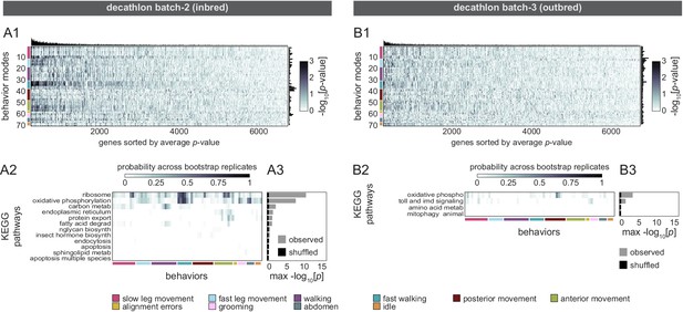
Correlation between individual transcriptomes and unsupervised behavioral measures.
(A1–B3) Gene expression characterization, modeling, and KEGG pathway enrichment for the second inbred (A1–A3) and outbred (B1-B3) Decathlon experiments. (A1–B1) Heatmaps of linear model -log p-values. Colored bars (left) indicate manual groupings of unsupervised behavioral measures by anatomical region (rows). Bar graphs show the number of significant (p<0.05) models for each gene (top) and behavior (right). (A2–B2) Heatmaps showing the probability across bootstrap replicates of a KEGG pathway being significantly enriched in the list of predictive genes for a given behavior. We did not observe any significant enrichment of KEGG pathways among genes predictive of distilled matrix principal components (PCs). (A3–B3) Bar plot showing the average across bootstrap replicates of the maximum (across behaviors) negative log adjusted p-value of all enriched KEGG pathways. Color indicates results from observed (gray) or shuffled control (black) data.
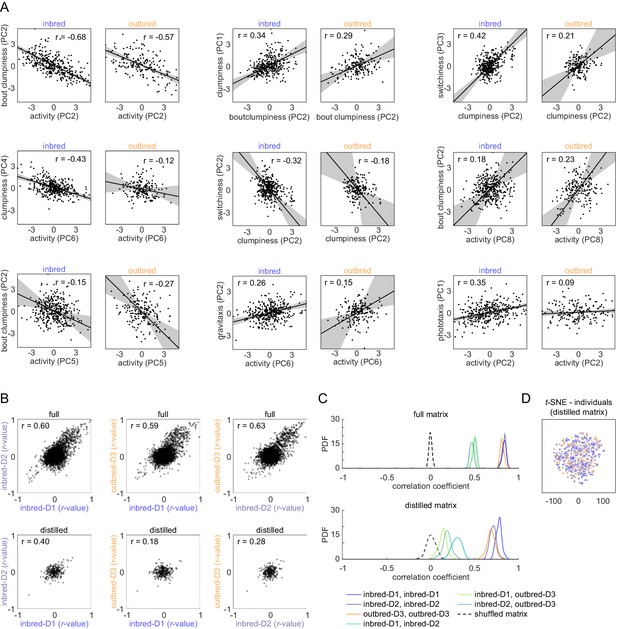
Comparison of inbred and outbred correlations.
(A) Example scatter plots of distilled matrix behavioral measures, in both inbred (left) and outbred (right) flies, with similar correlation coefficients. Black lines and shaded regions respectively indicate the line of best fit and 95% confidence intervals as estimated by bootstrap replicates of principal component analysis (PCA). (B) Scatter plots of full (top row) and distilled (bottom row) correlation matrix values across Decathlon iterations. The correlation of all correlation coefficients is indicated in the upper-left corner. (C) Kernel density estimates of the correlation of correlation matrix values in the Decathlon iterations. Distributions reflect variation in the estimate of the correlation under bootstrap resampling. (D) t-SNE embedding of individual flies from their representation in the 38-dimension distilled matrix to two dimensions. As in (A) and (B), blue indicates inbred flies and orange outbred.
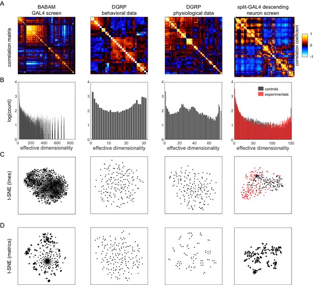
Analysis of Drosophila behavioral covariation in other non-isogenic populations.
(A) Correlation matrices of previously published data sets. Rows correspond to analyses performed on each data set. From left to right, the data sets (columns) are as follows: line averages of supervised behavioral classifications following thermogenetic inactivation in the fly olympiad screen (Robie et al., 2017), line averages of behavioral phenotypic data from wild-type inbred lines in the Drosophila Genomic Reference Panel (DGRP) database, line averages of physiological phenotypic data from the DGRP database, line averages of the fold change in unsupervised behavioral classifications following optogenetic activation of descending neurons (Cande et al., 2018). (B) Connected components spectra for each correlation matrix (see Materials and methods). Color in the rightmost plots (B–D) indicates either control (Gal4 driver only) or experimental animals (Gal4 × dTrapA1). (C) Points corresponding to lines nonlinearly embedded using t-SNE from the D-dimensional raw measure space to two dimensions (from left to right, d = 871, 31, 77, 151). (D) Points corresponding to lines nonlinearly embedded using t-SNE from the n-dimensional raw measure space to two dimensions (from left to right, n = 2083, 169, 169, 176).
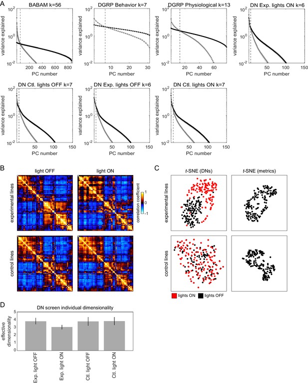
Structure of behavioral variation in non-Decathlon data sets.
(A) Scree plots showing the variance explained for each principal component (PC) of the BABAM Gal4 screen, Drosophila Genome Reference Panel (DGRP; behavioral and physiological), and descending neuron screen (all experimental groups and conditions) behavioral data sets. Point colors indicate variance explained for the observed (gray) and shuffled (black) data matrices. The dashed line indicates a simple metric of dimensionality (k), where the variance explained of the observed PCs is below the 95% confidence interval (shaded regions) of the shuffled data. (B) Correlation matrices for the combined behavioral probability density function (PDF) for each descending neuron set separated by experimental group and condition. (C) t-SNE embeddings of the descending neurons lines (left) and unsupervised measures (right) from the descending neuron screen. Color of the data points in the left-hand plot indicates whether individuals were control (black; Gal4/+) or experimental (red; Gal4/UAS-CsChrimson). (D) Average dimensionality k (as measured by the intersection of observed and shuffled ranked PC variances) of the individual behavioral PDFs separated by experimental group and condition. Error bars are the 95% confidence interval of the mean.
Videos
Examples of a mode of walking behavior as identified by the unsupervised analysis, from movies of single flies, made up of successive frames classified as the same behavior.
Colored dots indicate whether flies are outbred (NEX; red) or inbred (Berlin-Kiso; blue).
Examples of a mode of wing grooming behavior as identified by the unsupervised analysis, from movies of single flies, made up of successive frames classified as the same behavior.
Colored dots indicate whether flies are outbred (NEX; red) or inbred (Berlin-Kiso; blue).
Examples of a mode of head grooming behavior as identified by the unsupervised analysis, from movies of single flies, made up of successive frames classified as the same behavior.
Colored dots indicate whether flies are outbred (NEX; red) or inbred (Berlin-Kiso; blue).
Examples of a mode of abdomen flexing behavior as identified by the unsupervised analysis, from movies of single flies, made up of successive frames classified as the same behavior.
Colored dots indicate whether flies are outbred (NEX; red) or inbred (Berlin-Kiso; blue).
Additional files
-
Supplementary file 1
Details of Decathlon behavioral assays.
Assays varied in the number of metrics collected, with all assays including measurement of at least one metric repeated in another assay. In total, the assays featured four distinct arena geometries and three distinct experiment durations ranging from 15 min to 21 hr. A minimum activity criteria was applied to individuals for inclusion in the analysis from each assay, with the specific criteria depending on which metric most closely approximated activity for any particular assay.
- https://cdn.elifesciences.org/articles/64988/elife-64988-supp1-v1.xlsx
-
Supplementary file 2
Breakdown of a priori groups (group name, measures in each group, number of measures in each group, number of principal components [PCs] kept from each group, variance explained by kept PCs).
- https://cdn.elifesciences.org/articles/64988/elife-64988-supp2-v1.xlsx
-
Supplementary file 3
Decathlon assay behavioral measure details.
List of all assay behavioral measure names, definitions, numeric range, calculation, assay, a priori group, and inclusion criteria used to assign behavioral measures to their a priori group. Inclusion criteria used to form a priori groups were as follows: (1) multiple measures of the same metric in the same assay across days such as circadian speed days 1–10, (2) multiple measures of the same metric across assays such as Y-maze hand clumpiness and olfaction hand clumpiness, (3) metrics that likely share a trivial coupling such as LED Y-maze bout length and LED Y-maze choice number (i.e., longer average movement bouts resulting in more traversals through the arena center), (4) measures of responses to similar stimuli such as the three phototactic measurements in the LED Y-maze, temporal shade-light, and spatial shade-light assays, and (5) a priori group formed by a single measure due to none of the previous criteria applying.
- https://cdn.elifesciences.org/articles/64988/elife-64988-supp3-v1.xlsx
-
Supplementary file 4
List of Gal4 lines grouped by the cell types they target from the thermogenetic Shibirets and dTRPA1 screen.
Targeted neurons varied in the number of lines tested.
- https://cdn.elifesciences.org/articles/64988/elife-64988-supp4-v1.xlsx
-
Supplementary file 5
Decathlon enriched KEGG pathways for all Decathlon experiments.
Class and subclass correspond to KEGG pathway primary and secondary class terms. Observed p-value is the minimum adjusted p-value of the pathway enrichment across all behavioral metrics in the observed data (see Materials and methods details). Average minimum p-value is the mean of such p-values across bootstrap replicates. Gene hits and predictive genes correspond to the number and list of genes associated with the KEGG pathway in the observed data.
- https://cdn.elifesciences.org/articles/64988/elife-64988-supp5-v1.xlsx
-
Transparent reporting form
- https://cdn.elifesciences.org/articles/64988/elife-64988-transrepform1-v1.pdf


