Mechanical heterogeneity along single cell-cell junctions is driven by lateral clustering of cadherins during vertebrate axis elongation
- Department of Molecular Biosciences, University of Texas, United States
- Department of Chemistry, University of Texas, United States
- Department of Chemistry and Physics, Augusta University, Georgia
Figures
Figure 1 with 3 supplements
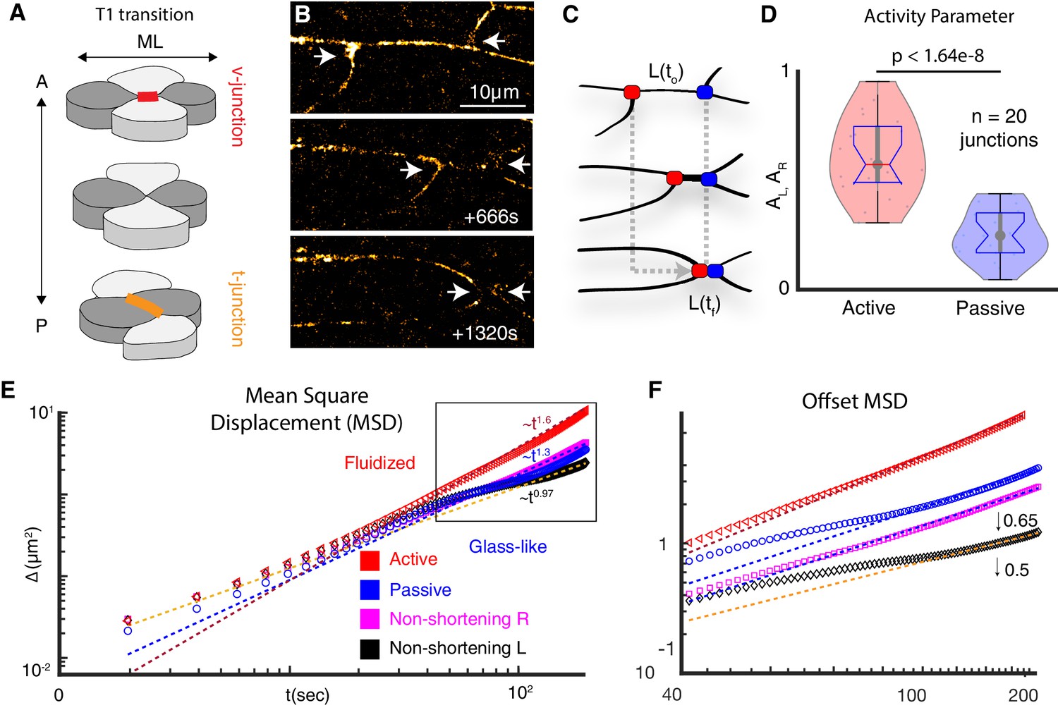
Vertices bounding shortening v-junctions are physically asymmetric and display heterogeneous fluid and glass-like dynamics.
(A) A four cell T1 transition with mediolaterally (ML)-aligned ‘v-junctions’ (red) and anterior-posterior (A/P) aligned t-junctions (orange) indicated. (B) Frames from time-lapse showing vertex movements of a v-junction; arrows highlight vertices. Frames were acquired at a z-depth of 5 μm above the ECM/coverslip and with a time interval of 2 s. (C) Schematic of asymmetric vertex movements from B; active = red; passive = blue. (D) Vertex motion quantified by the activity parameter, as described in Appendix, Section 1. (N = 42 vertices from 20 embryos; t-test p value is shown). (E) MSD reveals active vertices’ persistent superdiffusive movement (red); passive vertices exhibit intermediate time slowdown (blue). Pink and black display MSD for left and right non-shortening junctions. MSD is described in Appendix, Section 2. (F) MSD from boxed region in E is shown with traces offset for clarity (0.5 for left; 0.65 for right)(N = 20 vertices from 10 embryos).
Figure 1—figure supplement 1
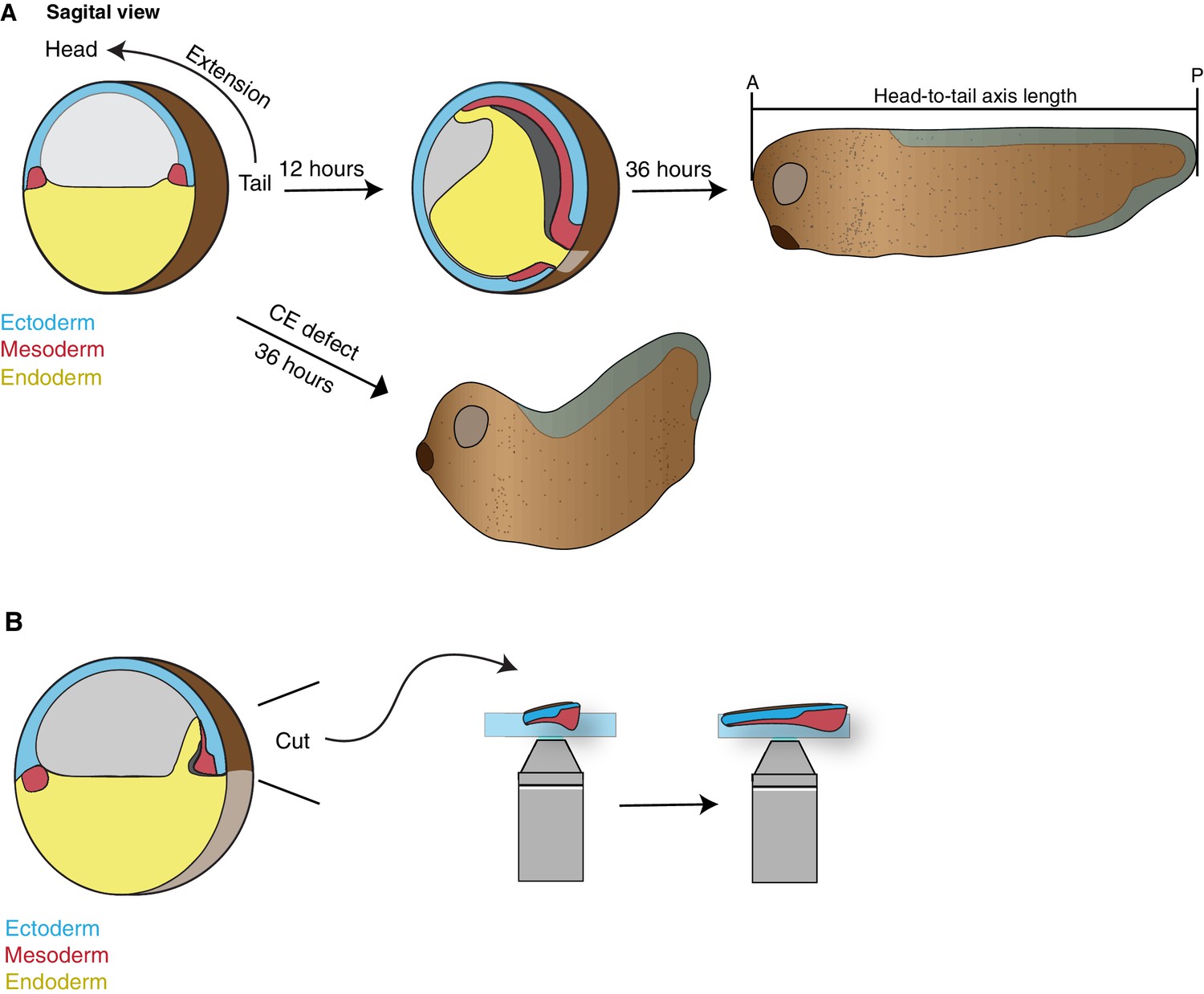
Schematics of Xenopus development.
(A) Cartoon depiction of Xenopus gastrulation, tadpole axis elongation, and the consequence of convergent extension defects. Here the mesoderm in the dorsal marginal zone (DMZ) involutes and undergoes convergent extension to establish the animals anterior-posterior (head-to-tail) axis. This axis will then continue to elongate during tadpole stages. Disruption of CE results in stunted embryos with a classic ‘swayed back’ appearance (lower arrow). (B) Classic embryological techniques were used to excise the DMZ (Keller explant) allowing visualization of CE in real-time.
Figure 1—figure supplement 2
Mean squared displacement measured from multiple frames of reference.
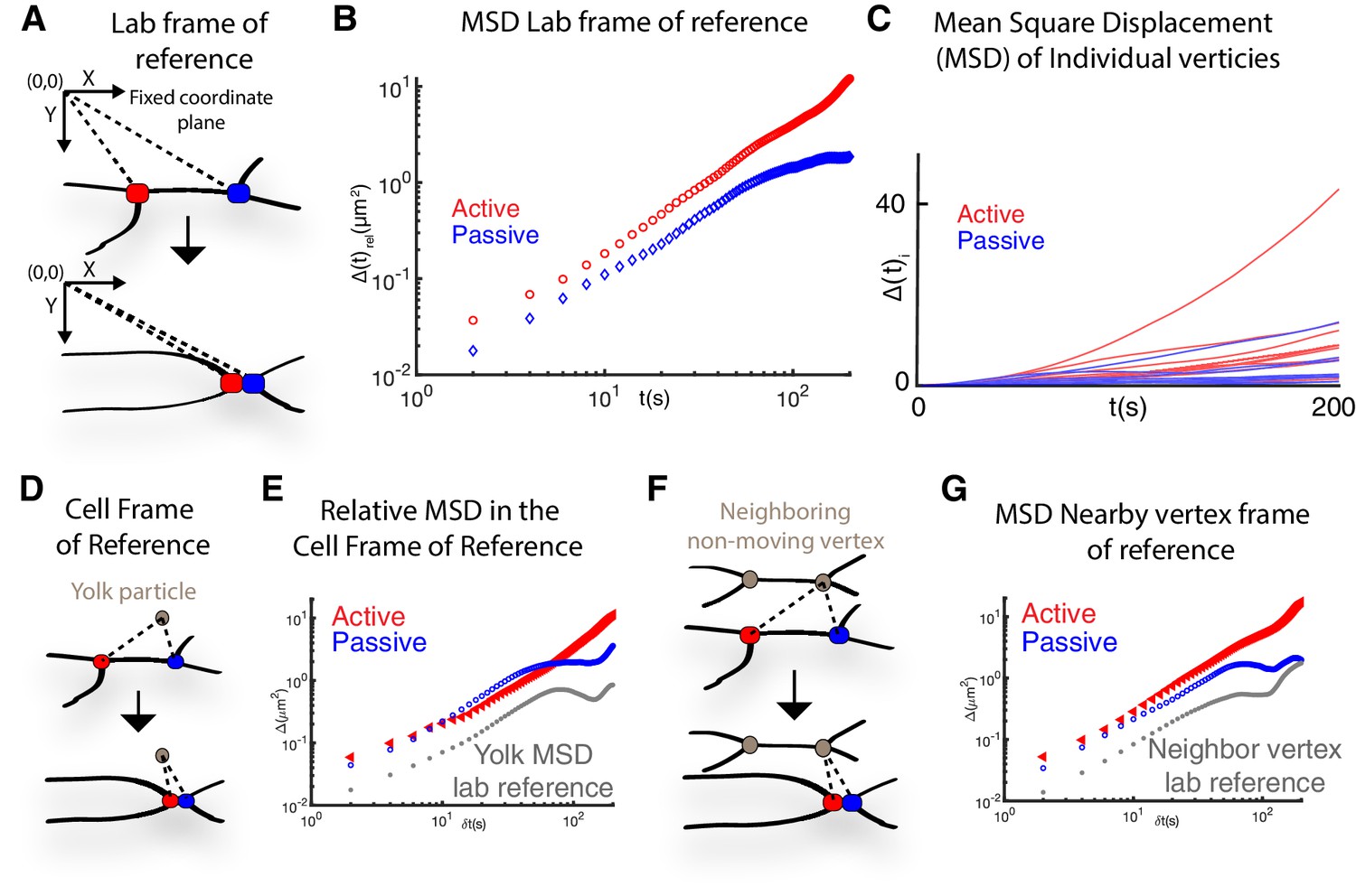
Appendix, Section 1. (A) Schematic showing how vertex MSD was measured from the lab frame of reference. Here the coordinate plane was set with the upper left corner of the image as (x,y)(0,0) and the pixels of the image were used as a fixed coordinate plane to measure the MSD. (B) Mean squared displacement of a pair of active and passive vertices in the lab frame of reference. (C) Mean squared displacements (MSD),, of 10 distinct individual active (red) and passive (blue) vertices. The heterogeneity in individual vertex movements is apparent from the wide variation in individual vertex MSDs. See for details on the MSD calculation. (D) Schematic showing how vertex mean square displacement was measured relative to yolk particles that are present in the embryonic Xenopus cells. We refer to this as the relative MSD in the cell frame of reference. (E) Relative mean squared displacement, , of vertices with respect to a yolk particle within a cell (cell frame of reference). Also included is the yolk particle MSD, calculated from the lab frame of reference (gray), to show minimal movement of the yolk compared to the vertices. (F) Schematic showing how vertex mean square displacement was measured relative to a neighboring vertex from other cells. This is the MSD in the nearby vertex frame of reference. (G) Relative mean squared displacement, , of the same pair of active and passive vertices in B (above) with the displacement analyzed relative to a nearby quasi-stationary vertex. The neighboring vertex MSD is also included as calculated from the lab frame of reference (gray).
Figure 1—figure supplement 3
Extended analysis of vertex glass-like dynamics.
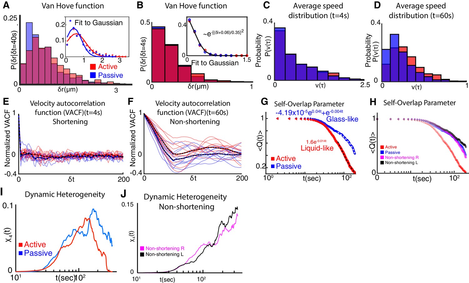
(A) Probability distribution of active (red) and passive (blue) vertex displacements, referred to as the van Hove function (see Equation 4 in Appendix Section 2), shows distinct non-Gaussian functional form. Inset shows deviation of the van Hove function from fits to Gaussian function for the active vertex and for the passive vertex. Probability distribution of distances moved over a time scale of , clearly shows the enhanced distance moved by active vertices as compared to passive vertices. Probability distribution is obtained for 20 individual vertices from 10 embryos. (B) Van Hove distribution of active (red) and passive (blue) vertex displacements at . Van Hove distribution for both active and passive vertices are well fit by a Gaussian distribution indicative of normal diffusive movement at short time scales. (C) Average vertex speed distribution for active (red) and passive (blue) vertices at (Appendix, Section 2). The speed distribution peaks at low values of average speed and rapidly decays of zero, showing similar trends for both active and passive vertices at . (D) Average vertex speed distribution for active (red) and passive (blue) vertices at . The distribution peaks at intermediate values of average speed. The active vertex speed distribution decays slower for larger values of the average velocity as compared to passive vertices. This is indicative of enhanced movement of active vertices. (E) Velocity autocorrelation function (VACF) for active (red) and passive (blue) vertices at (Appendix, Section 2). Active and passive vertex velocity autocorrelation rapidly decay to zero over a time scale of ~. Individual vertex correlations are plotted as solid lines. Mean is plotted as dashed lines. Active and vertex velocity correlations are similar in time at a short time interval, . (F) Velocity autocorrelation function (VACF) for active (red) and passive (blue) vertices at (Appendix, Section 2). Active vertex velocity is more persistent in time at this longer time interval compared to the passive vertex velocity. VACF quantifies the emergence of persistent motion of the active vertex at . The persistence time of the velocity correlation is over . (G) The self-overlap parameter, as quantified by decays slower for passive vertices (blue) as compared to active vertices (red). (H) For non-shortening vertices (magenta, black), the overlap parameter decays slower compared to active vertices (red). The overlap decays to 0 in the time interval probed for active vertices. The decay in the self-overlap parameter for passive vertices are comparable to non-shortening left and right vertices. See Appendix, Section 3 for further details. (I) The four-point susceptibility, , is calculated from the moments of with peaks visible for both active and passive vertices. (J) for non-shortening left (black) and right (magenta) vertices do not show a peak in the time frame analyzed. See Appendix, Section 3 for further details on the calculation of four-point susceptibility.
Figure 2 with 1 supplement

A new vertex model incorporating local mechanical heterogeneity recapitulates the fine-scale dynamics of junction shortening observed in vivo.
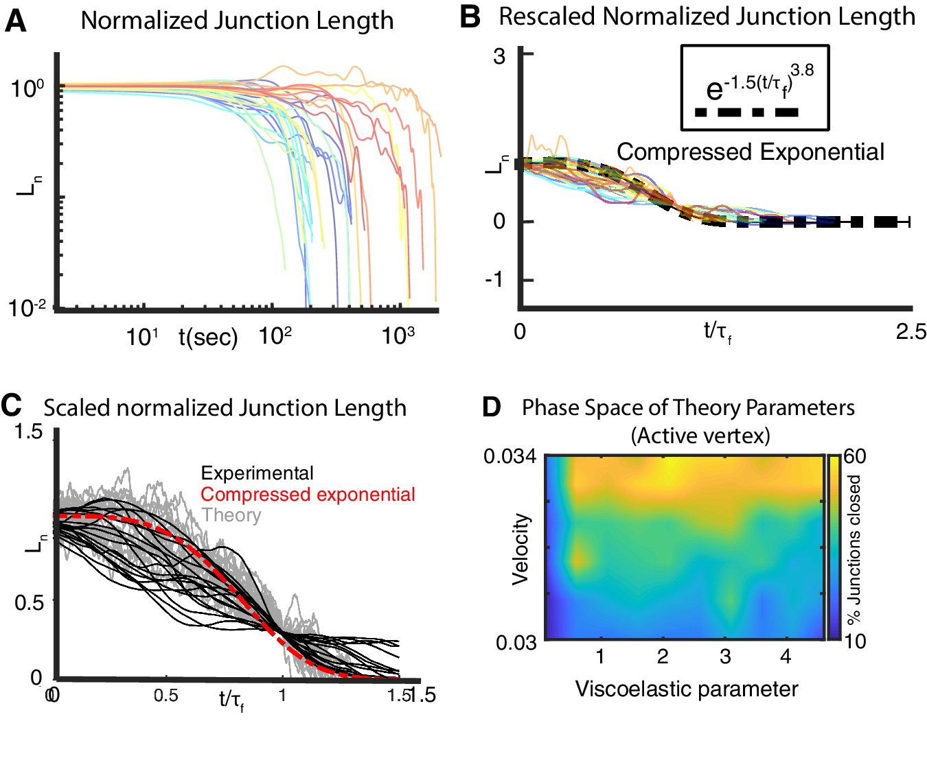
(A) Sketch of v- junction shortening with elements of the model overlain. Active (red) and passive (blue) vertex movements are affected by a piston modulating the dynamic rest length. The vertices execute elastic motion due to springs of elasticity, and . indices indicate left and right. The thicker spring indicates a stiffer elasticity constant, . (B) Equations of motion for active and passive vertex positions, and . Displacement of the left (right) vertex due to the piston is determined by the forces whose time dependence is determined by the rest length exponent,. The friction experienced by the left (right) vertices are modeled using is the colored noise term for the left vertex (Appendix, Section 4-6). (C) Heatmap indicating probability of successful junction shortening (legend at right) in parameter space for the viscoelastic parameter near vertices and the rest length exponent, staying within biologically reasonable values based on data from Drosophila (Solon et al., 2009; Appendix, Section 6). (D) Still image from a time-lapse of Xenopus CE. Insets indicate representative shortening and non-shortening junctions shown in Panels E and F (vertices indicated by arrowheads). (G) Normalized change in length, , for shortening junctions in vivo (black lines) and in simulations using asymmetric viscoelastic parameters (gray lines) resembling the compressed exponential form (red, dashed line) after the time axis is rescaled. (H) Normalized change in length, , for non-shortening junctions in vivo (black lines) and in simulations using symmetrical viscoelastic parameters (gray lines). (I) Quantification of relaxation behavior deviation from the compressed exponential using the residue (Appendix, Section 8-10).
Figure 2—figure supplement 1
Extended analysis comparing in vivo and in silico junction dynamics.
(A) C. Normalized relative change in length, , versus time for shortening mediolateral cell-cell junctions during CE. 21 individual junctions from 20 embryos are analyzed. and are the junction lengths at initial time and final time , respectively (Appendix, Section 9). (B) Although the normalized lengths vary considerably from one embryo to another, the nearly collapse onto a single universal curve (black dashed line) when the time axis is scaled by the relaxation time . The relaxation time is defined as This is evidence of the underlying self-similarity of the cell rearrangement process contributing to CE (Appendix, Section 9). (C) Comparison between experimental (black) and theoretical (gray) normalized junction length vs time for shortening junction shows that the model captures experimentally observed features of junction shortening during convergent extension. (D) Phase diagram for an alternative model (Appendix, Section 11) of active versus passive vertex contribution to junction shortening. Instead of accelerating vertices, we consider the velocity of vertices to be constant. Active vertex velocity is taken to be larger than the passive vertex. Simulations using the alternative model tell us that the viscoelastic parameter controls junction shortening. Our conclusion on the importance of the viscoelastic parameter in effecting junction shrinking is independent of the details of the vertex dynamics.
Figure 3
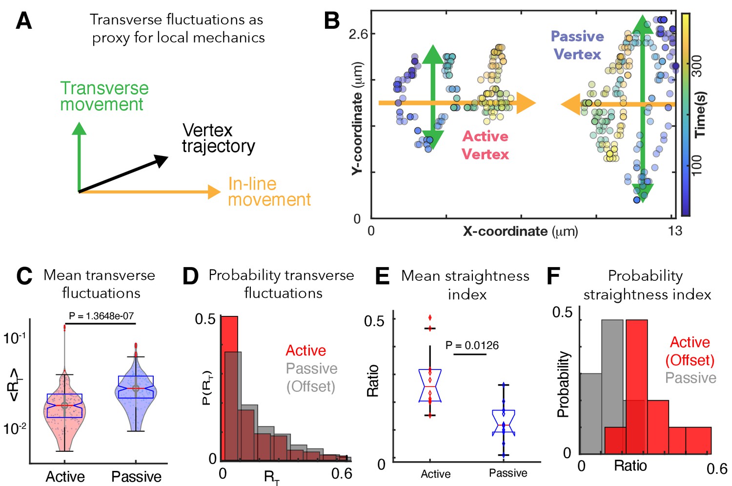
Patterns of transverse vertex fluctuations reveal mechanical heterogeneity of active and passive vertices in vivo.
(A) Schematic of transverse fluctuations in the vertex position perpendicular to the direction of junction shortening; traverse movements are extracted using the transverse 'hop' function, which is inversely proportional to the local vertex stiffness (Appendix, Section 12). (B) X/Y coordinates for a representative pair of active and passive vertices color coded for time, with transverse (green) and in-line (orange) motion indicated. (C) Mean transverse fluctuation , for active and passive vertices. (N=20 vertices; 10 embryos over 386 seconds; t-test p value shown). (D) Probability distribution of transverse fluctuations, , (offset for clarity). (E) Straightness index quantifying the persistence of vertex motion in terms of directionality (Appendix, Section 12); t-test p value is shown. (F) Probability distribution of the straightness index for active (red, offset for clarity) and passive (blue) vertices.
Figure 4 with 2 supplements
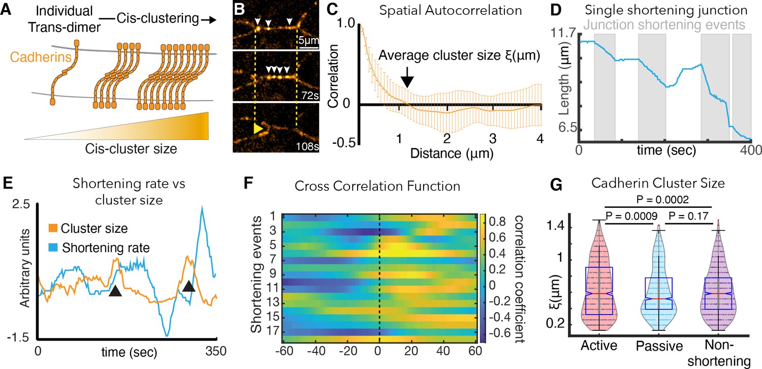
Cadherin cis-clustering correlates with vertex movements and mirrors asymmetric vertex dynamics.
(A) C-cadherin (Cdh3) cis-clustering; trans-dimers form across opposing cell membranes (gray); lateral cis interactions drive clustering. (B) Frames from time-lapse of Cdh3-GFP; white arrows highlight clusters. Dashed lines denote initial vertex positions; yellow arrow indicates junction shortening. (C) Spatial autocorrelation of Cdh3 intensity fluctuations (SI Section 13)(60 image frames, 10 embryos). Autocorrelation decays to zero at ~1 μm. Error bars are standard deviation. (D) Trace from a single v-junction displaying pulsatile shortening highlighted by gray boxes (E) Junction length and Cdh3 cluster size fluctuations for an individual cell-cell junction. Cadherin cluster size fluctuations peak prior to junction shortening events (Appendix, Section 14,15). (F) Heat map showing cross correlation between junction length and Cdh3 cluster size. Color represents the value of the correlation coefficient (legend at right). Dashed black line indicates zero lag time. (Appendix, Section 14,15)(n = 11 junctions and 18 shortening events.) (G) Cadherin cluster size as extracted from spatial correlation curves (Figure 4—figure supplement 2; Appendix, Section 16). Cadherin cluster sizes are significantly larger near active vertices. Clusters near vertices of non-shortening junctions are not significantly different from those near passive vertices.
Figure 4—figure supplement 1
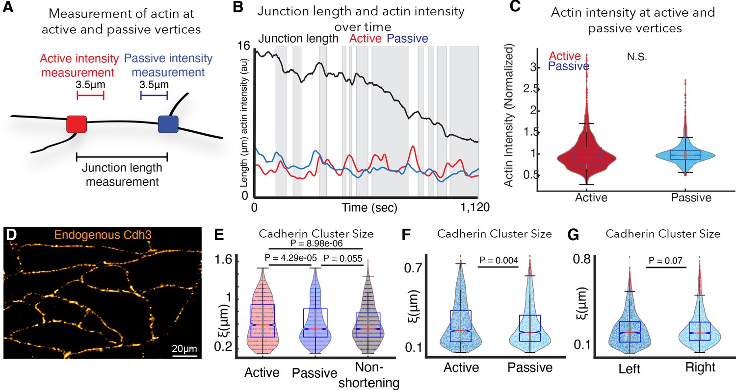
Extended analysis pertaining to cdh3 clustering and actin next to junctions (Appendix, Section 16).
(A) Schematic showing how actin was measured next to active and passive vertices at shortening v-junctions. (B) Graph showing junction length and actin intensities over time for a single shortening junction. The black line is junction length, red is actin intensity next to the active vertex, and blue is actin intensity next to the passive vertex. (C) Graph showing normalized actin intensity next to active (red) or passive vertices. Intensity was normalized to account for expression by dividing each datapoint by the mean intensity of the dataset. Conditions were statistically compared using a t-test. (D) Immunostaining for endogenous Cdh3 showing that the endogenous protein forms cadherin cis-clusters. (E) Violin plot of Cdh3 cluster sizes next to active vertices (red), passive vertices (blue), and non-shortening left and right vertices (black) for all frames including shortening and non-shortening events. Statistical significance was assessed using a Kolmogorov-Smirnov test. (F) An alternative definition of cluster size was used to analyze differences in cadherin clustering. By fitting an exponential function to the spatial autocorrelation of cadherin intensity fluctuation, we extract the characteristic cadherin cluster size. Violin plot shows the Cdh3 cluster sizes for active versus passive vertices in shortening junctions. 1538 frames from 10 embryos were analyzed. Kolmogorov-Smirnov shows significant differences between Cdh3 clustering near active versus passive vertices (p=0.004). (G) Violin plot of Cdh3 cluster sizes for left versus right vertices in non-shortening junctions. A total of 2062 frames from seven embryos were analyzed. Kolmogorov-Smirnov did not indicate significant differences between Cdh3 clustering near left versus right vertices (p=0.07).
Figure 4—figure supplement 2
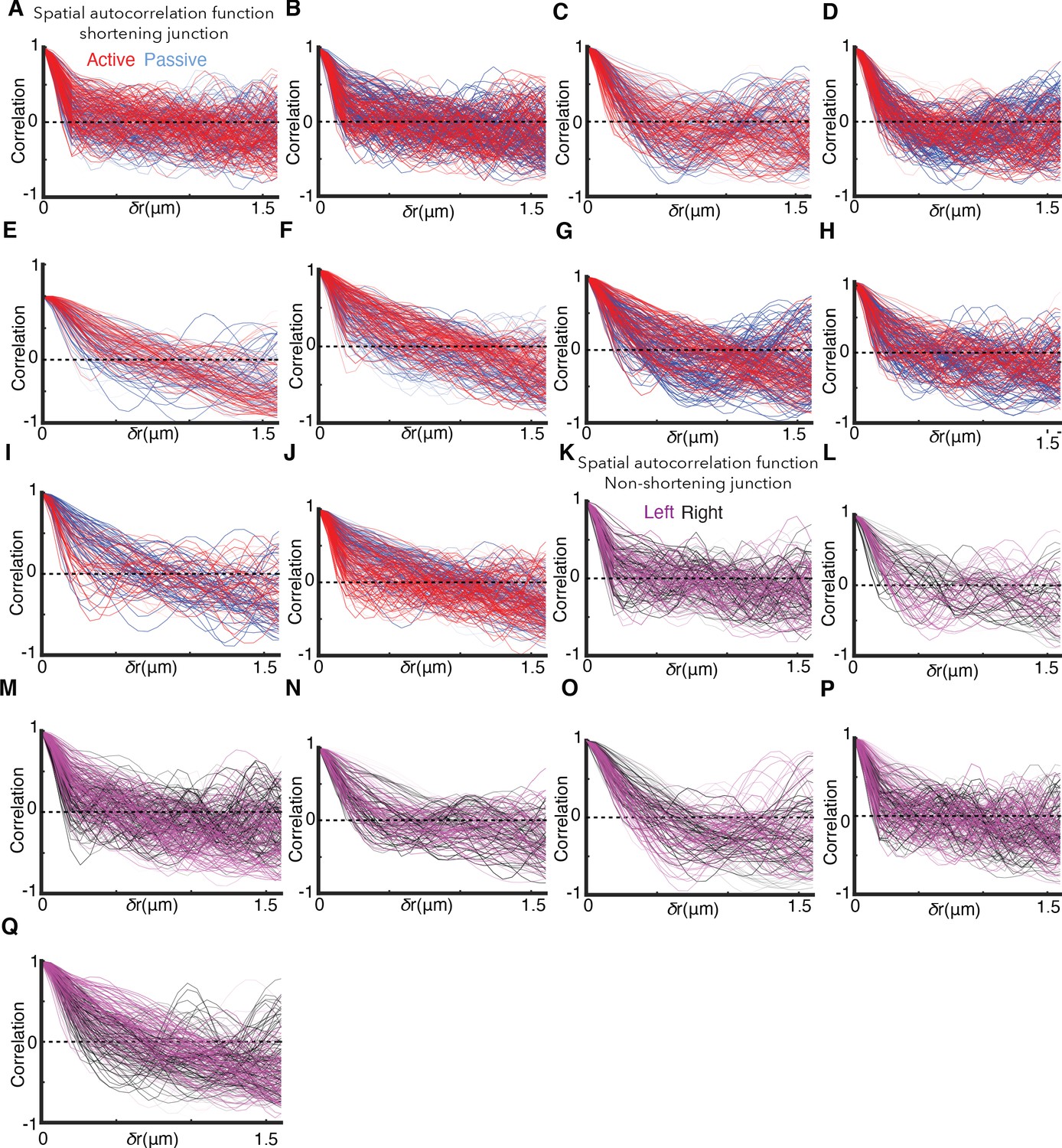
Source data for spatial correlation of Cdh3 intensity fluctuations reveal extreme heterogeneity in cluster size.
(A-J) Individual (time frame by frame) spatial correlation vs distance curves selecting for shortening events from 10 distinct cell-cell junctions that undergo successful junction shortening (Appendix, Section 16). Cadherin spatial correlation near active (passive) vertices are shown in red (blue) lines. (K-Q) Individual (time frame by frame) spatial correlation vs distance curves from seven distinct cell-cell junctions that do not successfully shorten. Cadherin spatial correlation near left (right) vertices are shown in magenta (black) lines (Appendix, Section 16).
Figure 5 with 1 supplement
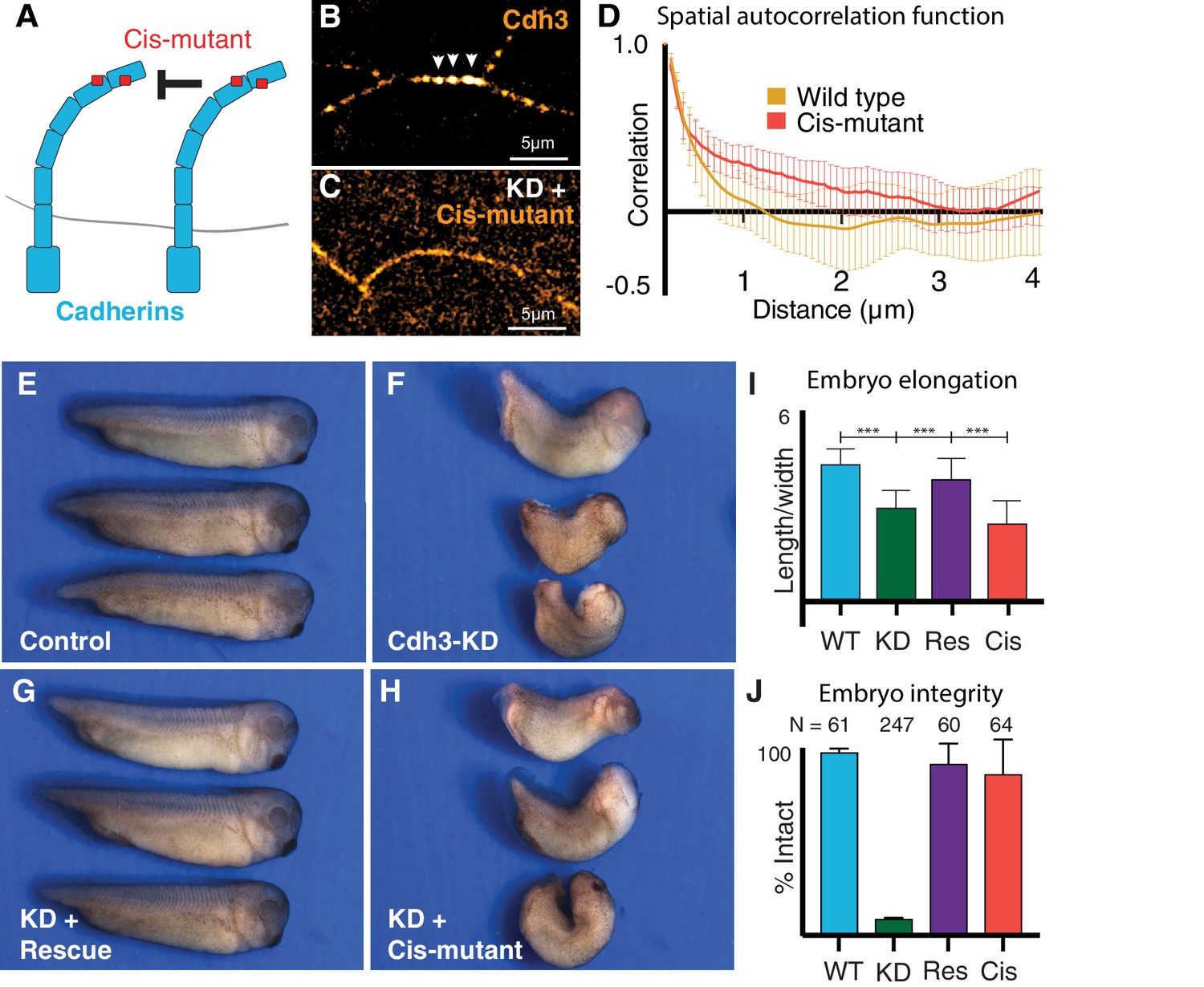
Cdh3 cis-clustering is required for convergent extension but not homeostatic tissue integrity.
(A) Mutations used to inhibit cadherin cis-clustering. (B) Cdh3-GFP clustering in a control embryo. (C) Cis-clusters absent after re-expression of cisMut-Cdh3-GFP. (D) Mean spatial autocorrelation of Cdh3-GFP intensity fluctuations for wild type (60 image frames, from 10 embryos) and the cis-mutant (56 image frames, five embryos) (Appendix, Section 17). Gradual, non-exponential decay for cisMut-Cdh3-GFP indicates a lack of spatial order (i.e. failure to cluster). (E) Control embryos (~stage 33). (F) Sibling embryos after Cdh3 knockdown. (G) Knockdown embryos re-expressing wild-type Cdh3-GFP. (H) Knockdown embryos re-expressing cisMut-Cdh3-GFP. (I) Axis elongation assessed as the ratio of anteroposterior to dorsoventral length at the widest point. (J) Embryo integrity assessed as percent of embryos alive and intact at stage 23.
Figure 5—figure supplement 1
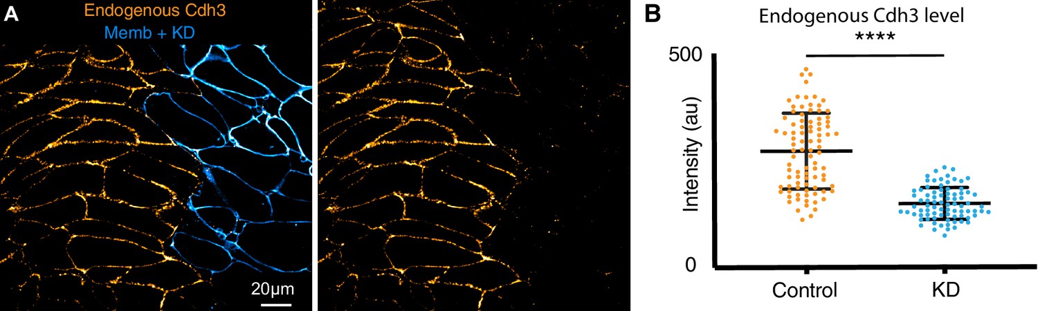
Cdh3 knockdown.
(A) Embryos were injected with Cdh3-MO and membrane-BFP in a single dorsal blastomere at the four-cell stage resulting in mosaic depletion of Cdh3. Here, immuno-staining for Cdh3 shows that the protein was depleted specifically in cells that received the morpholino, as marked by membrane-BFP. (B) Cdh3 immuno-staining intensity was measured in control cells and neighboring Cdh3-MO cells from mosaic animals. These data were derived from three replicate experiments and statistically analyzed by t-test.
Figure 6
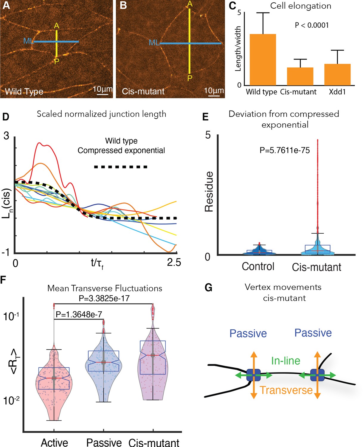
Cdh3 cis-clustering is required for heterogeneous junction mechanics.
(A) Image of polarized, elongated control Xenopus mesoderm cells. Blue = mediolateral (ML); yellow = anterior-posterior (AP). (B) Stage-matched cells after depletion of endogenous Cdh3 and re-expression of cisMut-Cdh3. (C) Cellular length/width ratio to quantify CE cell behaviors (p value indicates ANOVA result). (D) Normalized junction length dynamics () for cis-mutant expressing junctions. Large fluctuations here are similar to those seen normally in non-shortening junctions (see Figure 2H). Dashed black line indicates the expected compressed exponential. (E) The residue quantifying significant deviation from the compressed exponential function as compared to control junctions. (F) Plots for transverse fluctuations , for control active and passive vertices compared to cis-mutant vertices. (Note: Data for active and passive junctions are re-presented from Figure 3C for comparison.) (G) Schematic illustrating symmetrical vertex behavior after disruption of cdh3 cis-clustering.
Figure 7 with 1 supplement
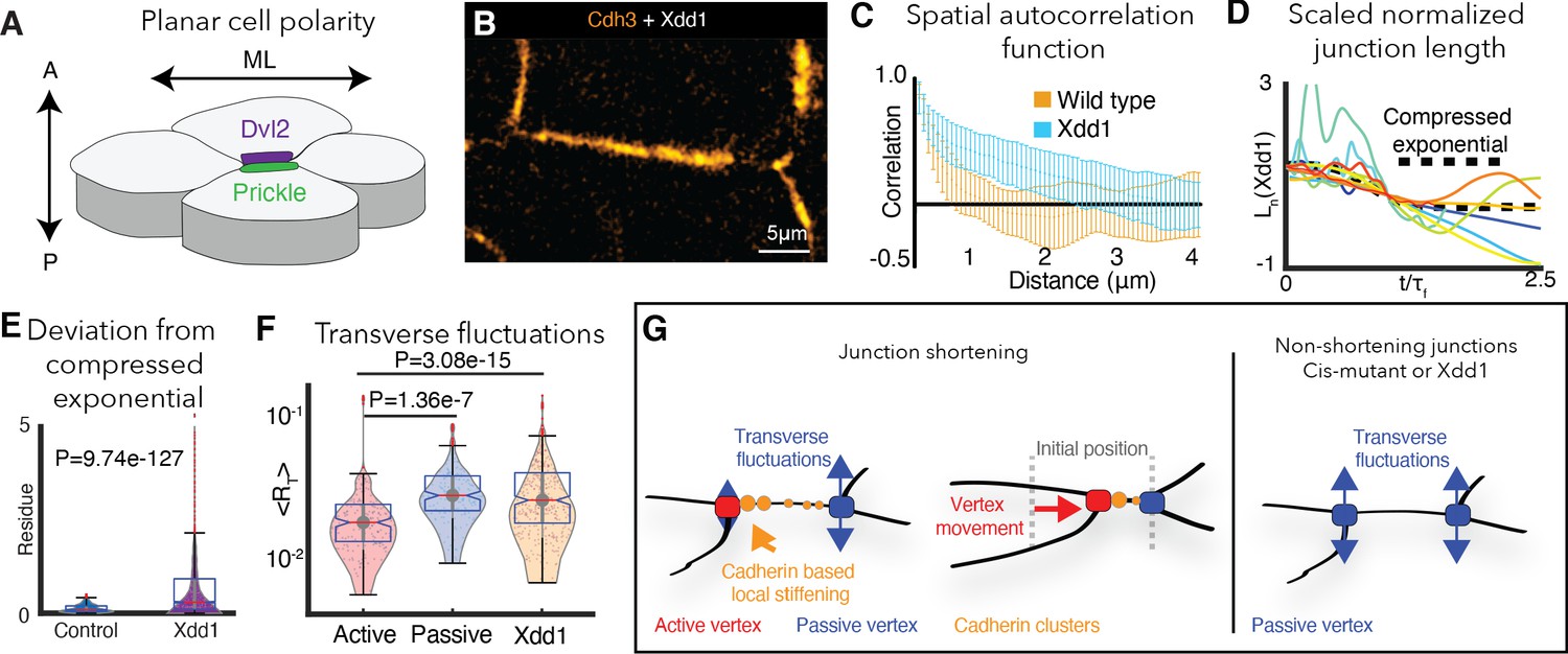
PCP is required for cdh3 cis-clustering and heterogeneous junction mechanics.
(A) Cartoon of polarized core PCP protein localization. (B) Still image of Cdh3-GFP after expression of dominant negative Dvl2 (Xdd1). (C) Spatial autocorrelation of Cdh3 intensity fluctuations for Xdd1 (53 image frames, 5 embryos) and control embryos (60 frames, from 10 embryos),± std. dev. The spatial organization of Xdd1 mutant cadherin is similar to cisMut-Cdh3 expressing embryos. (D) Normalized junction length dynamics for Xdd1 embryos. Dashed black line indicates the normal compressed exponential behavior. (E) Residue for the deviation from the universal compressed exponential function for Xdd1 junctions. (F) Plots for transverse fluctuations at active and passive vertices compared to Xdd1-expressing vertices. (Note: Data for active and passive junctions are re-presented from Figure 3C for comparison to Xdd1.) (G) Schematic summarizing the primary conclusions.
Figure 7—figure supplement 1
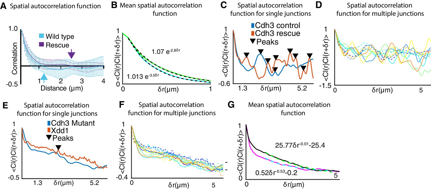
Extended analysis of cadherin clustering for the cis-mutant, rescue, and Xdd1.
(A) Spatial autocorrelation of Cdh3 intensity fluctuations for wild type (60 frames, obtained from 10 embryos) and Cdh3-rescue (58 frames, obtained from 4 embryos). The characteristic correlation length decays to zero at ~1 , for both wild type and rescue embryos. Error bar is the standard deviation. (B) Mean spatial autocorrelation of Cdh3 intensity fluctuations for wild type and rescue with functional fits to the decay behavior. Both spatial correlations can be fit to an exponential. This is evidence for a characteristic spatial scale for the correlation in spatial Cdh3 intensity fluctuations. (C) Single junction spatial autocorrelation of cadherin intensity fluctuations in Cdh3 wild type and rescue embryos. Local maxima in the Cdh3 spatial correlation are indicated as peaks (Appendix, Section 17). This shows the well-defined spatial periodicity in Cdh3 distribution along the cell-cell junction for both wild type and rescue embryos. (D) Spatial autocorrelation of cadherin intensity fluctuations in Cdh3 control (solid lines) and Cdh3 rescue (dashed lines) embryos along a single junction at five different time frames. (E) Single junction spatial autocorrelation of cadherin intensity fluctuations in Cdh3 mutant and Xdd1 mutant embryos. As compared to wild type and rescue embryos, local maxima in the Cdh3 spatial correlation is highly suppressed. The spatial periodicity of Cdh3 distribution along the cell-cell junction is not seen. (F) Spatial autocorrelation of cadherin intensity fluctuations in Cdh3 mutant (solid lines) and Xdd1 mutant (dashed lines) embryos along a single junction at five different time frames. (G) Mean spatial autocorrelation of Cdh3 intensity fluctuations for Xdd1(black) and Cdh3 mutant (magenta) with functional fits to the decay behavior. Both spatial correlations decay to zero is better fit to a power law. This is evidence for the lack of characteristic spatial scale for the correlation in spatial Cdh3 intensity fluctuations.
Additional files
Download links
A two-part list of links to download the article, or parts of the article, in various formats.
Downloads (link to download the article as PDF)
Open citations (links to open the citations from this article in various online reference manager services)
Cite this article (links to download the citations from this article in formats compatible with various reference manager tools)
Mechanical heterogeneity along single cell-cell junctions is driven by lateral clustering of cadherins during vertebrate axis elongation
eLife 10:e65390.
https://doi.org/10.7554/eLife.65390


