Figures and data in High infectiousness immediately before COVID-19 symptom onset highlights the importance of continued contact tracing | eLife

Figures
Additional files

4 figures and 2 additional files

Figures

Figure 1

Download asset Open asset

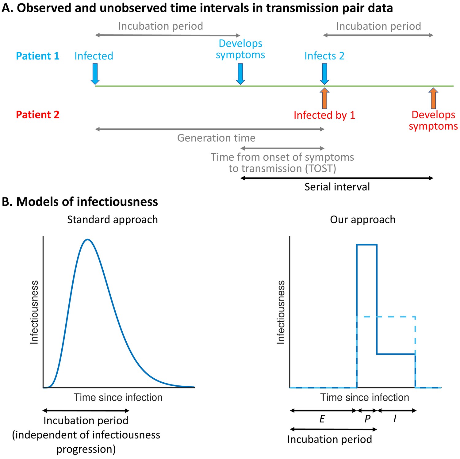
Schematic illustrating epidemiological time intervals in data from infector–infectee transmission pairs and approaches for inference from transmission pair data.

(A) Transmission pair data generally comprise symptom onset dates for known infector–infectee pairs. These data may be supplemented with partial information about infection times, consisting of a range of possible exposure dates for infectors and/or infectees (Ferretti et al., 2020a). While the serial interval for each pair can be calculated directly from the data (with some uncertainty, given the unknown precise times of symptom appearance on the onset dates [Thompson et al., 2019]), other time intervals, including the generation time and TOST, are unobserved (these are shown in grey). (B) In standard approaches (left panel) for inferring infectiousness profiles from transmission pair data, the infectiousness of a host at a given time since infection is assumed to be independent of their incubation period. In our approach (right panel), we link a host’s infectiousness with when they develop symptoms. We assume that individuals are not infectious during the latent (E) period and that infectiousness may either vary between the presymptomatic infectious (P) and symptomatic infectious (I) periods (solid line – this corresponds to our ‘variable infectiousness model’), for example due to changing behaviour in response to symptoms (Manfredi and D’Onofrio, 2013), or be identical in these two time periods (dashed line – this corresponds to our ‘constant infectiousness model’).

Figure 2 with 2 supplements

Download asset Open asset

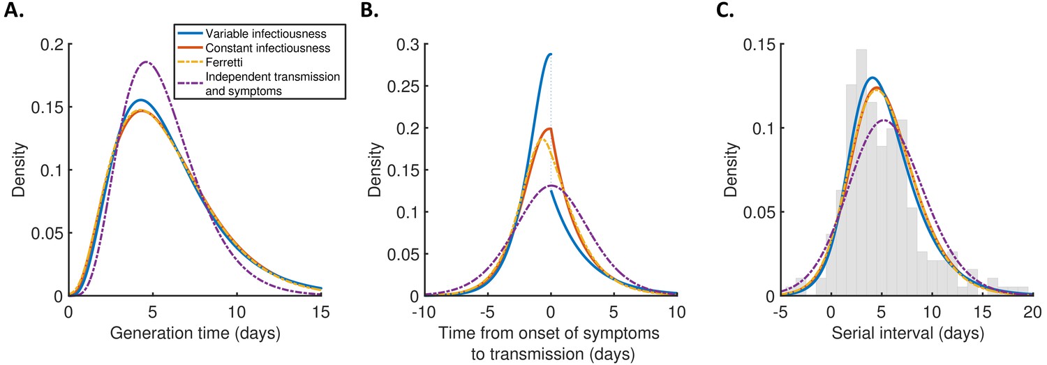
Distributions of epidemiological time intervals.

Distributions of epidemiological time intervals estimated by fitting different models to data from 191 SARS-CoV-2 transmission pairs (Figure 2—source data 1). (A) Generation time, indicating the relative expected infectiousness of a host at each time since infection. (B) Time from onset of symptoms to transmission (TOST), indicating the relative expected infectiousness of a host at each time since symptom onset. (C) Serial interval, indicating the periods between infectors and infectees developing symptoms. In (C), the empirical serial interval distribution from the transmission pair data (Figure 2—source data 1) is shown as grey bars. In addition, discretised versions of the serial interval distributions, calculated using the method in Cori et al., 2013, are shown in Figure 2—figure supplement 1. In all panels, lines represent: variable infectiousness model (blue), constant infectiousness model (red), Ferretti model (orange dashed), and independent transmission and symptoms model (purple dashed). We assumed a specified incubation period distribution (Lauer et al., 2020) when fitting the different models to data (see Materials and methods); equivalent panels using an alternative incubation period distribution (Linton et al., 2020) are shown in Figure 2—figure supplement 2.

Figure 2—source data 1 Transmission pair data. Data comprising symptom onset dates and (where available) intervals of possible exposure times in 191 SARS-CoV-2 infector–infectee pairs. These data were originally reported in five different studies (Ferretti et al., 2020a; He et al., 2020; Xia et al., 2020; Cheng et al., 2020; Zhang et al., 2020), and were previously compiled in Ferretti et al., 2020b.: https://cdn.elifesciences.org/articles/65534/elife-65534-fig2-data1-v2.xlsx
Download elife-65534-fig2-data1-v2.xlsx

Figure 2—figure supplement 1

Download asset Open asset

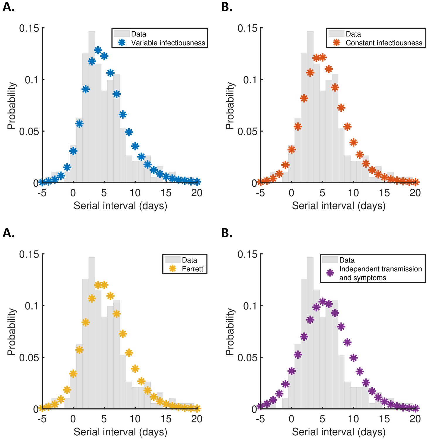
Discretised serial interval distributions.

Discretised versions of the serial interval distributions shown in Figure 2C, calculated using the method in Cori et al., 2013, plotted as stars alongside the empirical serial interval distribution from the transmission pair data (grey bars). (A) Variable infectiousness model. (B) Constant infectiousness model. (C) Ferretti model. (D) Independent transmission and symptoms model.

Figure 2—figure supplement 2

Download asset Open asset

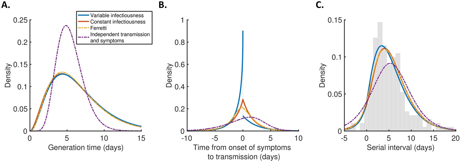
Robustness to the assumed incubation period distribution.

Equivalent panels to Figure 2 for an alternative incubation period distribution (Linton et al., 2020). ΔAIC values for the different models are 0 (variable infectiousness model), 5.1 (constant infectiousness model), 10.2 (Ferretti model), and 64.5 (independent transmission and symptoms model).

Figure 3 with 2 supplements

Download asset Open asset

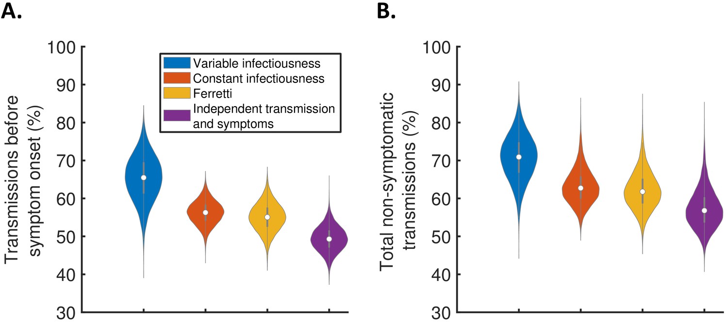
The contribution of non-symptomatic infectious individuals to transmission.

(A) Violin plots indicating posterior distributions for the proportion of transmissions occurring prior to symptom onset for individuals who develop symptoms (i.e., neglecting transmissions from individuals who remain asymptomatic throughout infection) for the different models. (B) Posterior distributions for the total proportion of non-symptomatic transmissions, accounting for transmissions from asymptomatic infectious individuals (Figure 3—figure supplement 1), for the different models. Equivalent panels assuming an alternative incubation period distribution (Linton et al., 2020) are shown in Figure 3—figure supplement 2.

Figure 3—figure supplement 1

Download asset Open asset

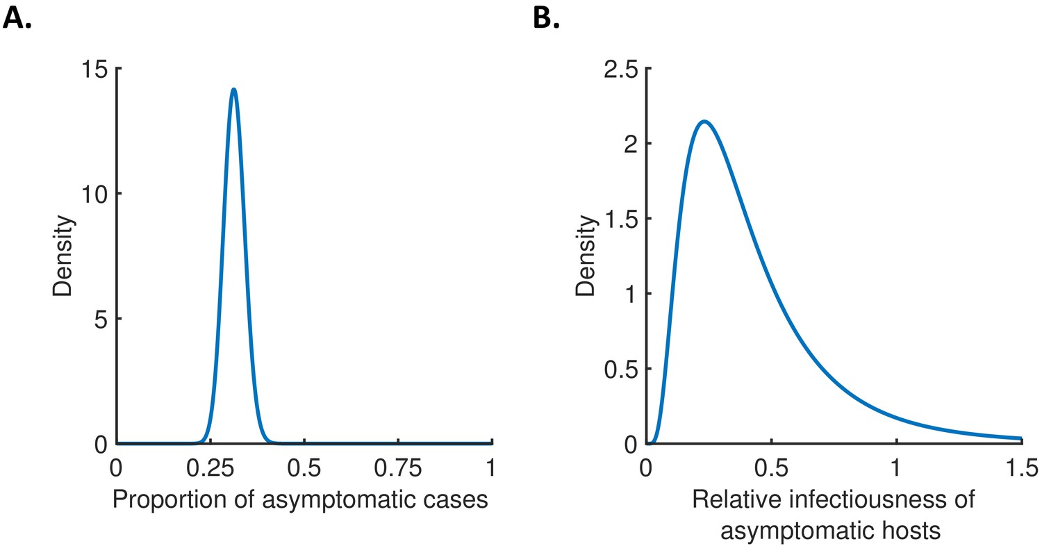
The contribution of asymptomatic cases to transmission.

(A) Assumed distribution for the proportion of asymptomatic cases, $p_{A}$ . (B) Assumed distribution for the relative infectiousness of asymptomatic hosts, $x_{A}$ . These distributions were chosen for consistency with the confidence intervals in (1) (Materials and methods).

Figure 3—figure supplement 2

Download asset Open asset

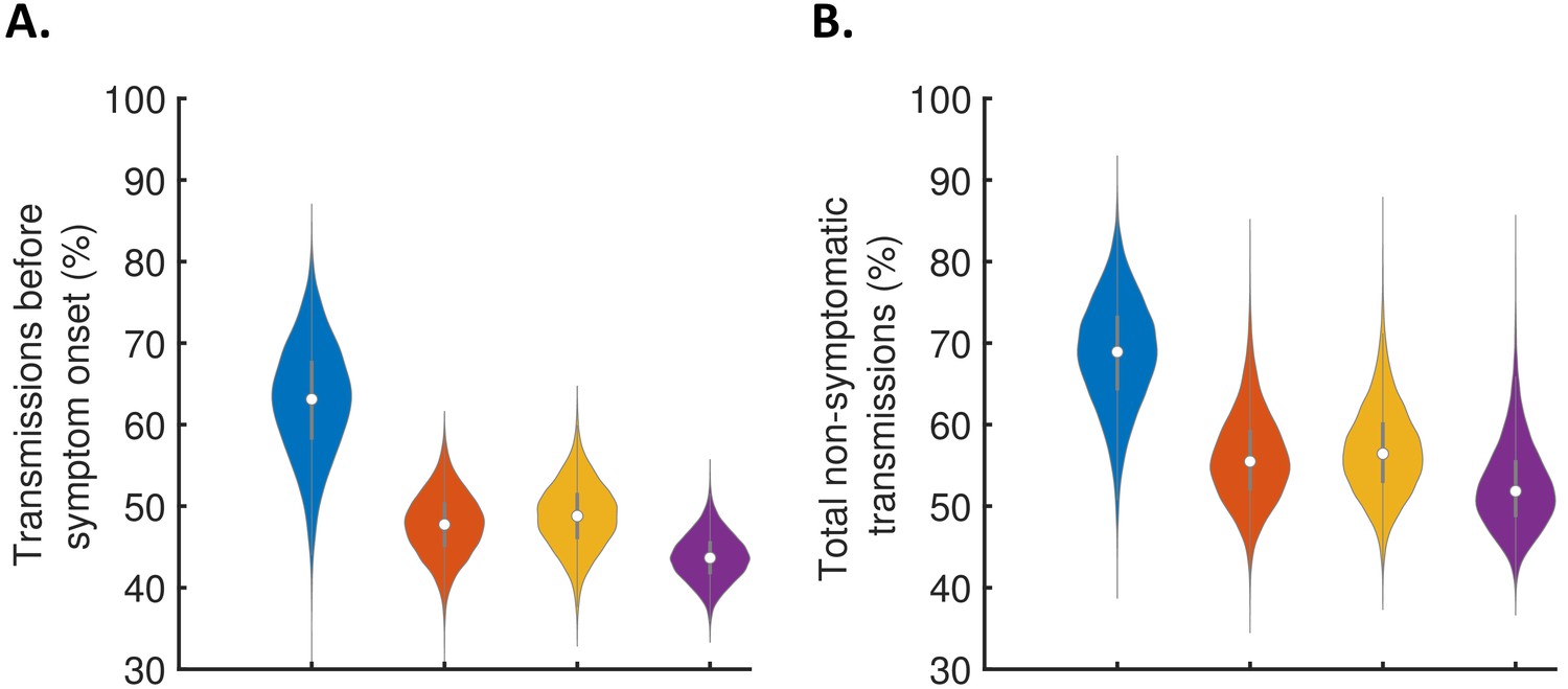
Robustness to the assumed incubation period distribution.

Equivalent panels to Figure 3 for an alternative incubation period distribution (Linton et al., 2020).

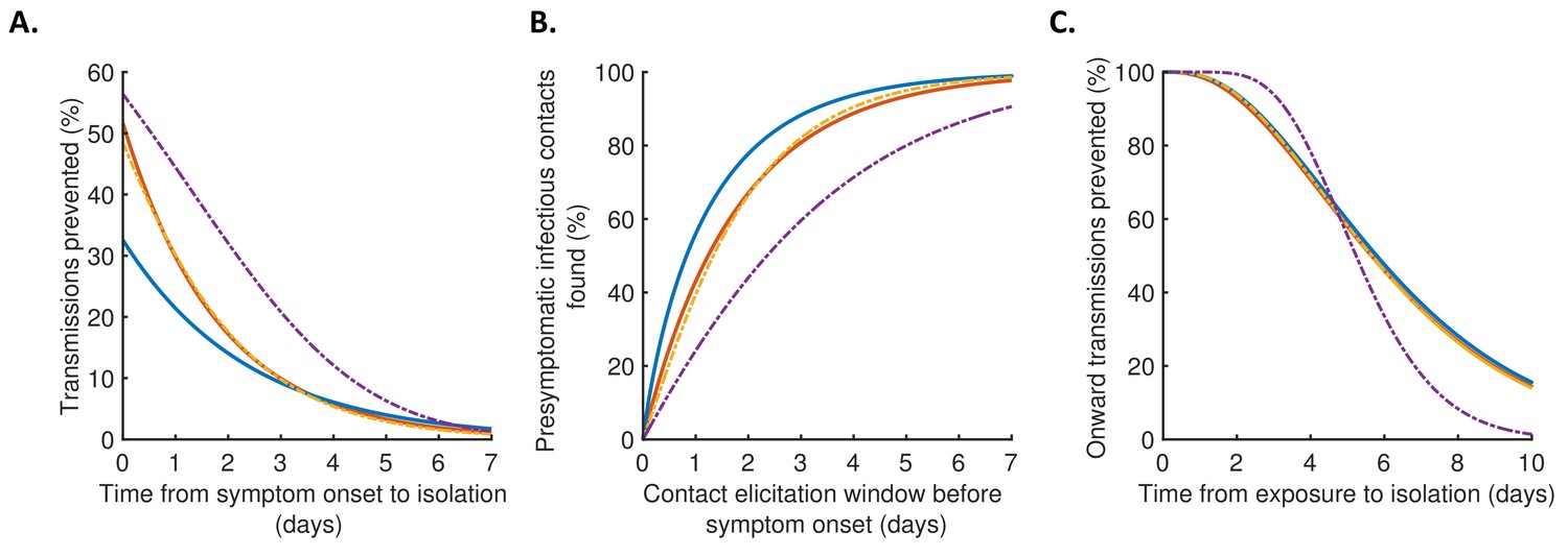
Figure 4 with 2 supplements

Download asset Open asset

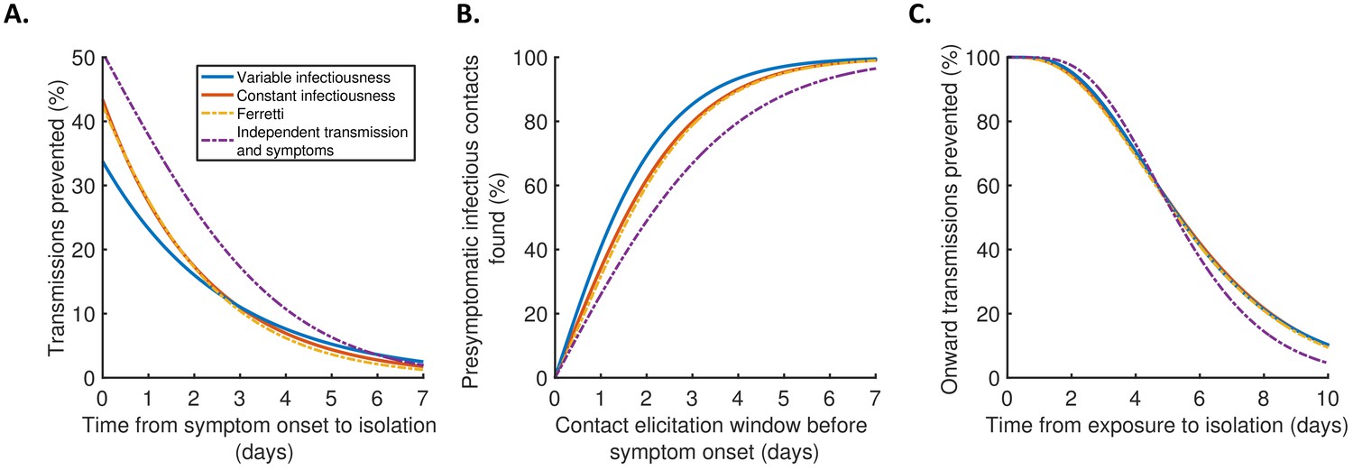
Implications for isolation and contact tracing.

(A) Effect of the timing of isolation of symptomatic index cases: the proportion of transmissions prevented through isolation, for different time periods between symptom onset and isolation. (B) Effect of the contact elicitation window: the proportion of presymptomatic infectious contacts found for different times up to which contacts are traced before the symptom onset time of the index host. (C) Effect of the timing of isolation of infected contacts: the proportion of onward transmissions generated by the contacts prevented by isolation of those contacts, for different time periods between exposure to the index host and isolation of the contacts. In all panels, lines represent predictions obtained using point estimate parameters for the variable infectiousness model (blue), constant infectiousness model (red), Ferretti model (orange dashed), and independent transmission and symptoms model (purple dashed). Here, isolation and contact tracing are assumed to be 100% effective; equivalent panels in which the effectiveness is less than 100% are shown in Figure 4—figure supplement 1. Equivalent panels assuming an alternative incubation period distribution (Linton et al., 2020) are shown in Figure 4—figure supplement 2.

Figure 4—figure supplement 1

Download asset Open asset

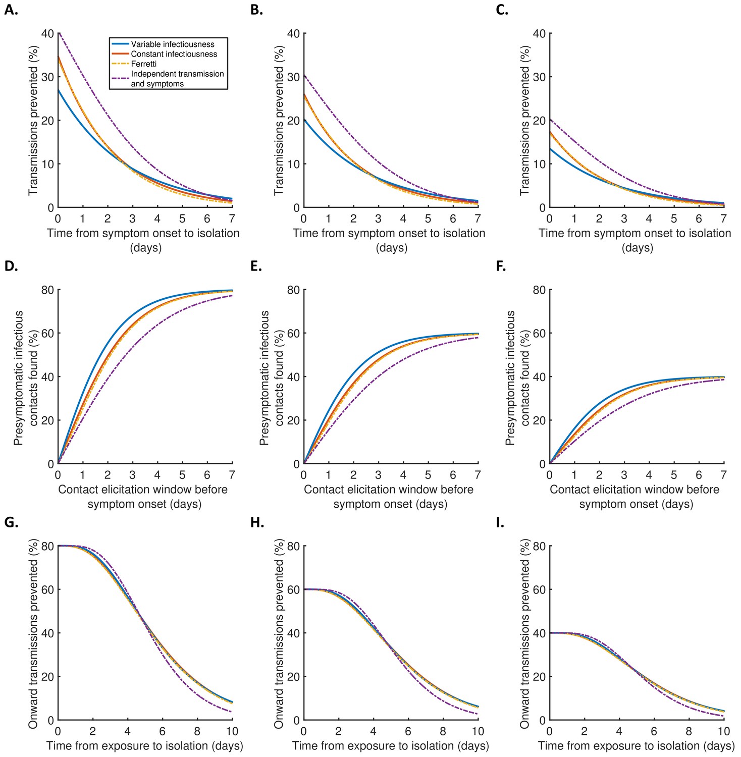
Robustness to effectiveness of contact tracing and isolation.

(A–C) Equivalent panels to Figure 4A for different values of the isolation effectiveness, $ε_{1}$ (see Materials and methods). (A) $ε_{1} = 0.8$ . (B) $ε_{1} = 0.6$ . (C) $ε_{1} = 0.4$ . (D–F) Equivalent panels to Figure 4B for different values of the contact identification effectiveness, $ε_{2}$ (see Materials and methods). (D) $ε_{2} = 0.8$ . (E) $ε_{2} = 0.6$ . (F) $ε_{2} = 0.4$ . (G–I) Equivalent panels to Figure 4C for different values of the contact isolation effectiveness, $ε_{3}$ (see Materials and methods). (G) $ε_{3} = 0.8$ . (H) $ε_{3} = 0.6$ . (I) $ε_{3} = 0.4$ .

Figure 4—figure supplement 2

Download asset Open asset

Robustness to the assumed incubation period distribution.

Equivalent panels to Figure 4 for an alternative incubation period distribution (Linton et al., 2020).

Additional files

Supplementary file 1 Table of fitted parameter values. Point estimates (obtained by calculating the posterior mean of the vector of fitted parameters, $θ$ , as described in Materials and methods) and 95% credible intervals for fitted parameters are given for each model. Note that the parameters $μ_{F}$ and $α_{F}$ in the Ferretti model do not have the same epidemiological interpretations as the parameters $μ$ and $α$ in our mechanistic approach.: https://cdn.elifesciences.org/articles/65534/elife-65534-supp1-v2.docx
Download elife-65534-supp1-v2.docx
Transparent reporting form: https://cdn.elifesciences.org/articles/65534/elife-65534-transrepform-v2.docx
Download elife-65534-transrepform-v2.docx

Download links

A two-part list of links to download the article, or parts of the article, in various formats.

Downloads (link to download the article as PDF)

Open citations (links to open the citations from this article in various online reference manager services)

Mendeley

Cite this article (links to download the citations from this article in formats compatible with various reference manager tools)

William S Hart
Philip K Maini
Robin N Thompson

(2021)

High infectiousness immediately before COVID-19 symptom onset highlights the importance of continued contact tracing

eLife 10:e65534.

https://doi.org/10.7554/eLife.65534

Sign up for email alerts

Privacy notice