Figures and data in Dynamic decision policy reconfiguration under outcome uncertainty

Figures
Tables
Additional files

23 figures, 3 tables and 1 additional file

Figures

Figure 1

Download asset Open asset

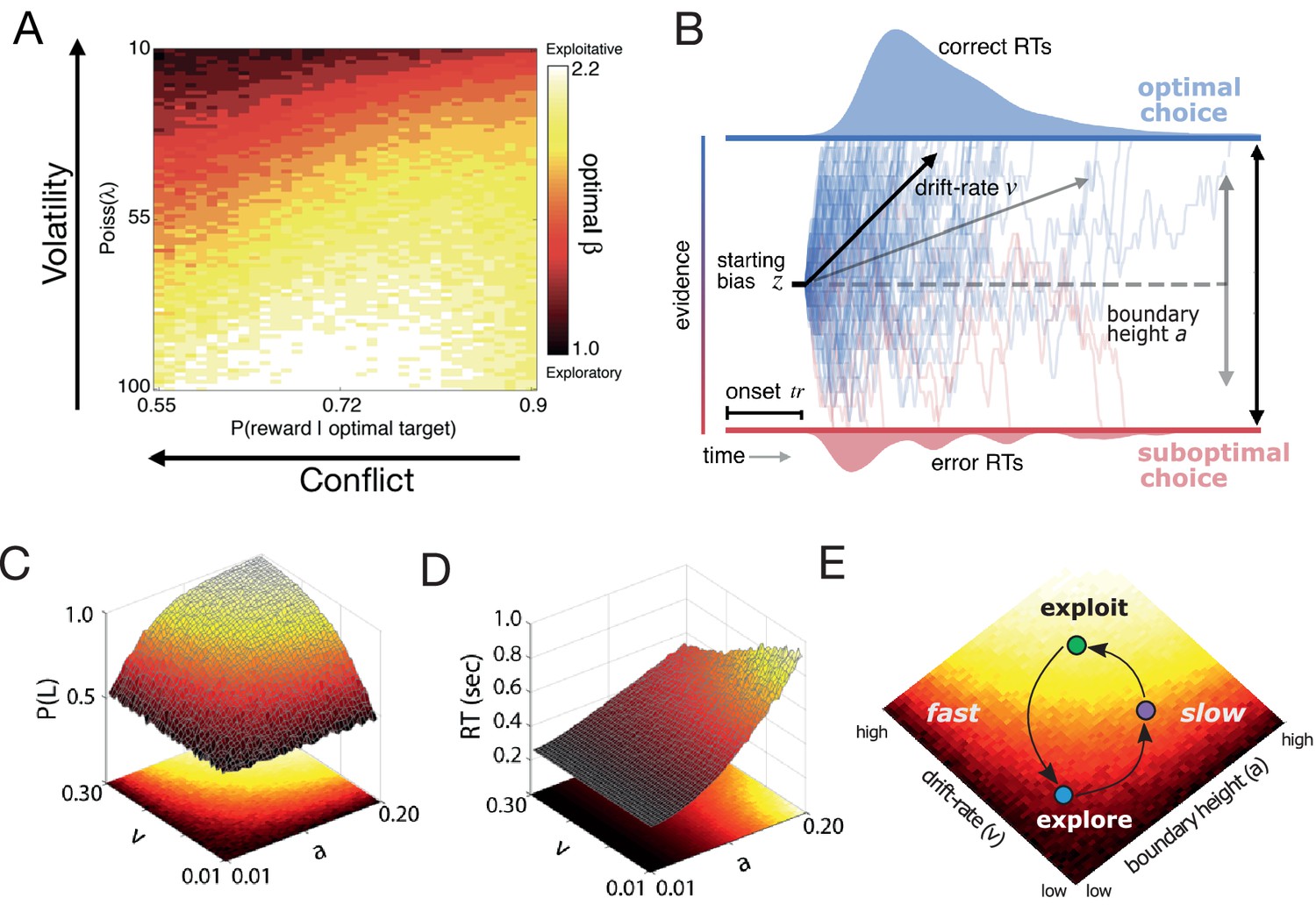
Dynamic decision policy reconfiguration.

(A) The degree of conflict and volatility shifts the optimal balance between exploration and exploitation. (B) The drift diffusion model. (C) Accuracy (probability that left choice selected is selected; P(L)) as a function of coordinated changes in the rate of evidence accumulation (v) and the amount of information needed to make a decision, or the boundary height (a). (D) Reaction time as a function of changes in the rate of evidence accumulation and the boundary height. (E) Decision policy reconfiguration.

Figure 2

Download asset Open asset

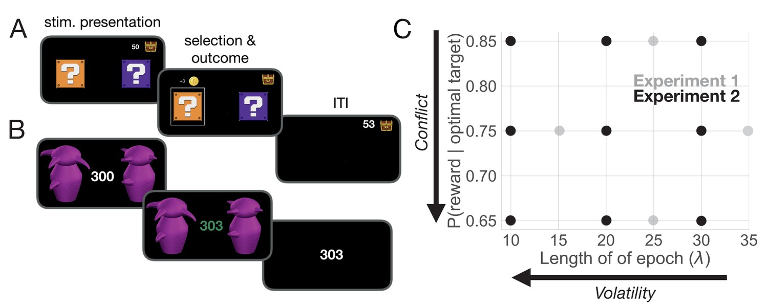
Task and uncertainty manipulation.

(A) In Experiment 1, participants were asked to choose between one of two ‘mystery boxes’. The point value associated with a selection was displayed above the chosen mystery box. The sum of points earned across trials was shown to the left of a treasure box on the upper right portion of the screen. (B) In Experiment 2, participants were asked to choose between one of two Greebles (one male, one female). The total number of points earned was displayed at the center of the screen. The stimulus display was rendered isoluminant throughout the task. (C) The manipulation of conflict and volatility for Experiments 1 (gray) and 2 (black). Each point represents the combination of degrees of conflict and volatility. Under high conflict, the probability of reward for the optimal and suboptimal target is relatively close. Under high volatility, a switch in the identity of the optimal target selection is relatively frequent.

Figure 3

Download asset Open asset

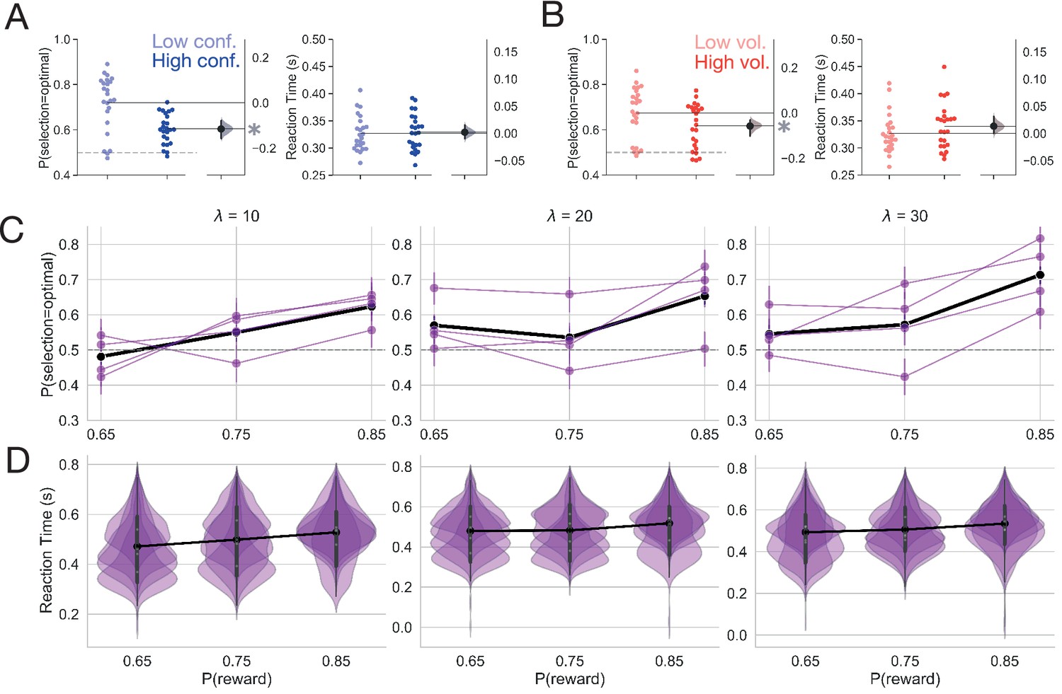
Behavior.

(A) Mean accuracy and reaction time for the manipulation of conflict in Experiment 1. (B) Mean accuracy and reaction time for the manipulation of volatility in Experiment 1. Each point represents the average for a single subject. The distribution to the right represents the bootstrapped uncertainty in the mean difference between conditions (high conflict or high volatility subtracted from low conflict or low volatility). Distributions with 95% CIs that do not encompass 0 are marked with an asterisk. (C) Mean accuracy for Experiment 2. Each purple line represents a subject. The black line represents the mean accuracy calculated across subjects. (D) Reaction time distributions for each subject for Experiment 2. The black line represents the mean reaction time calculated over subjects. Error bars indicate a bootstrapped 95% confidence interval. For panels C and D, $λ$ values shown above each plot specify the average period of optimal choice stability and the probability of reward shown on the x-axis specifies the degree of conflict. Means are calculated over all trials.

Figure 4

Download asset Open asset

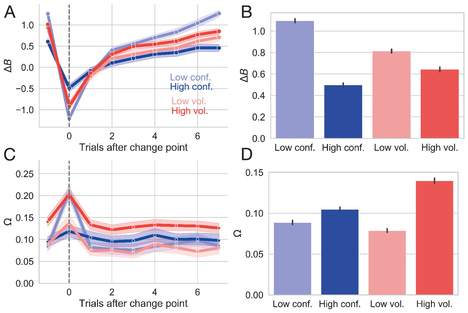
Changes in ideal observer estimates as a function of condition for Experiment 1.

(A) Changes in the belief in the value of the optimal target ( $Δ B$ ) as a function of conflict and volatility over time. (B) Belief in the value of the optimal choice by condition and averaged over all trials. (C) Changes in change point probability ( $Ω$ ) as a function of conflict and volatility over time. (D) Change point probability by condition and averaged over all trials. Error bars represent 95% CIs.

Figure 5

Download asset Open asset

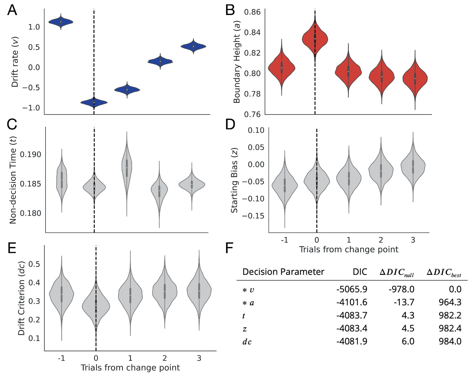
Change point sensitivity of underlying decision processes.

Posterior distributions for each decision parameter are shown for the trial prior to a change point to three trials after the change point. (A) The drift rate. (B) The boundary height. (C) Non-decision (onset) time. (D) Starting bias. (E) Drift criterion. (F) Degree of fit to observational data as information loss. The models that lost the least information are marked with an asterisk.

Figure 6

Download asset Open asset

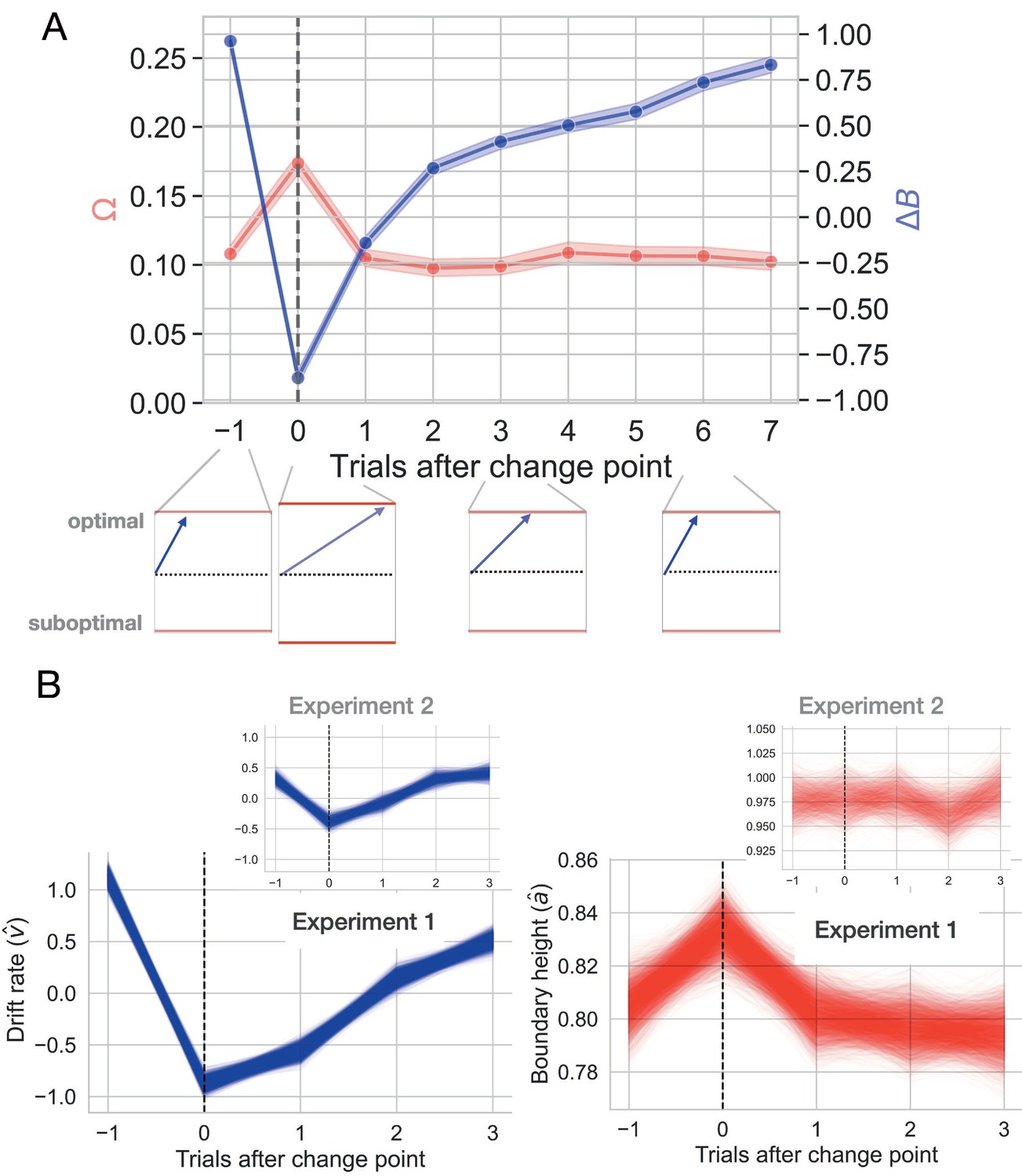
Change-point-evoked uncertainty.

(A) Changes in ideal observer estimates of uncertainty over time and their effect on the boundary height and the drift rate. Directly after a change point, the boundary height *increases* and the drift rate slows. Over time, the boundary height returns to its baseline value and the drift rate increases. (B) Fitted estimates of change-point-evoked drift rate and boundary height for both experiments with 95% CIs of the posterior distributions. Inset plots represent data from Experiment 2.

Figure 7

Download asset Open asset

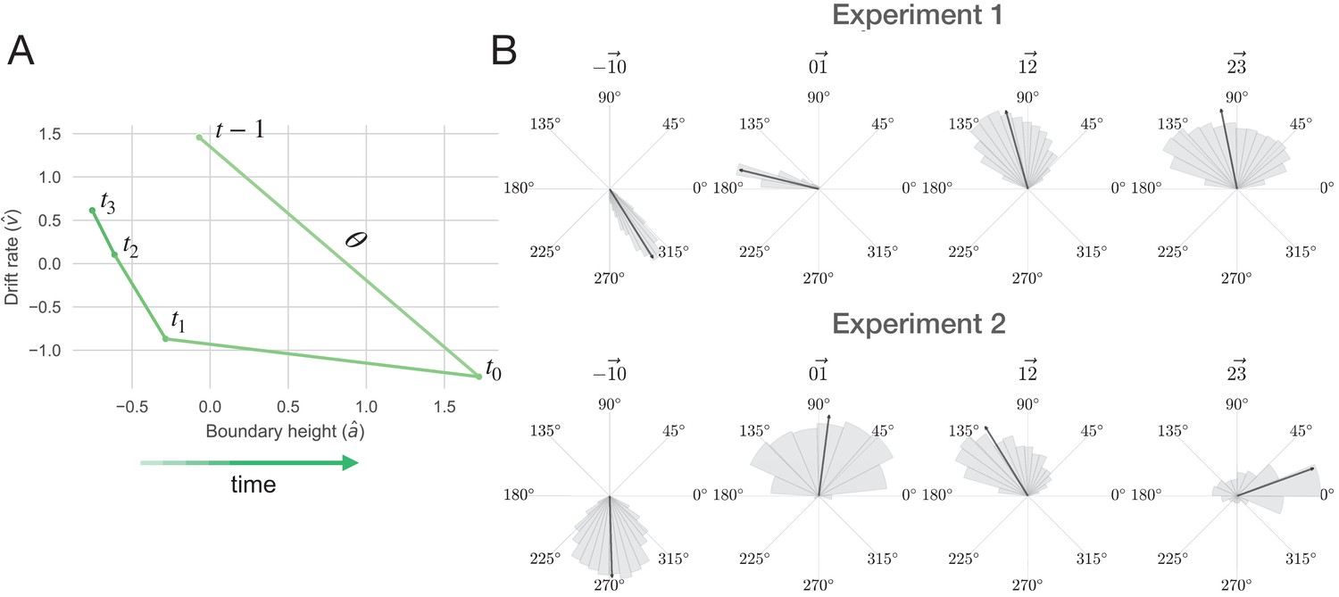
The decision surface.

(A) Representing decision space in vector form. An angle ( $θ$ ) was calculated between sequential values of ( $a$ , $v$ ) coordinates, beginning with the trial prior to the change point. This represents subject-averaged data from Experiment 1. Note that these trajectories are z-scored. (B) Distributions depicting the angle between drift rate and boundary height for both Experiments 1 and 2. Each subpanel shows the distribution of angles between ( $a$ , $v$ ) over sequential trials, beginning with the trial prior to the change point. The area of the shaded region is proportional to the density and the arrow represents the circular mean.

Figure 8

Download asset Open asset

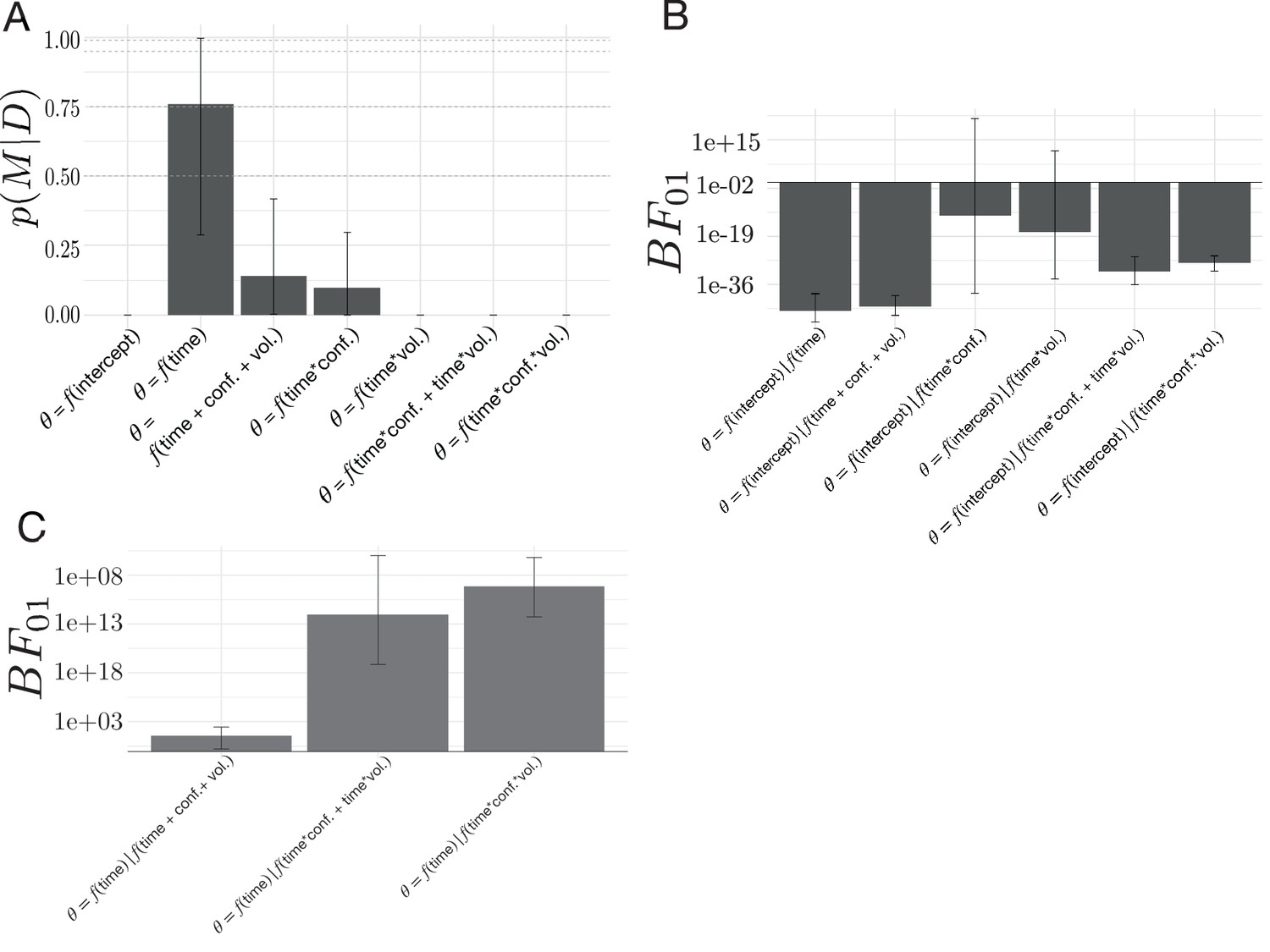
Model comparisons for the effect of volatility and conflict on the relationship between drift rate and boundary height.

(A) The posterior probability for models testing for an effect of volatility and conflict on the angle of shift in $a$ and $v$ , $θ$ . (B) The Bayes Factor for the null model relative to the alternative models specifying either an effect of time relative to a change point alone or a conditional effect on this evoked response $θ$ . (C) The Bayes Factor for the evoked response model relative to the surviving alternative models specifying a conditional effect on the evoked response, $θ$ . Note that time refers to time relative to the onset of a change point. All models specifying an interaction also include main effects. Dotted horizontal lines refer to grades of evidence (Wagenmakers, 2007).

Figure 9

Download asset Open asset

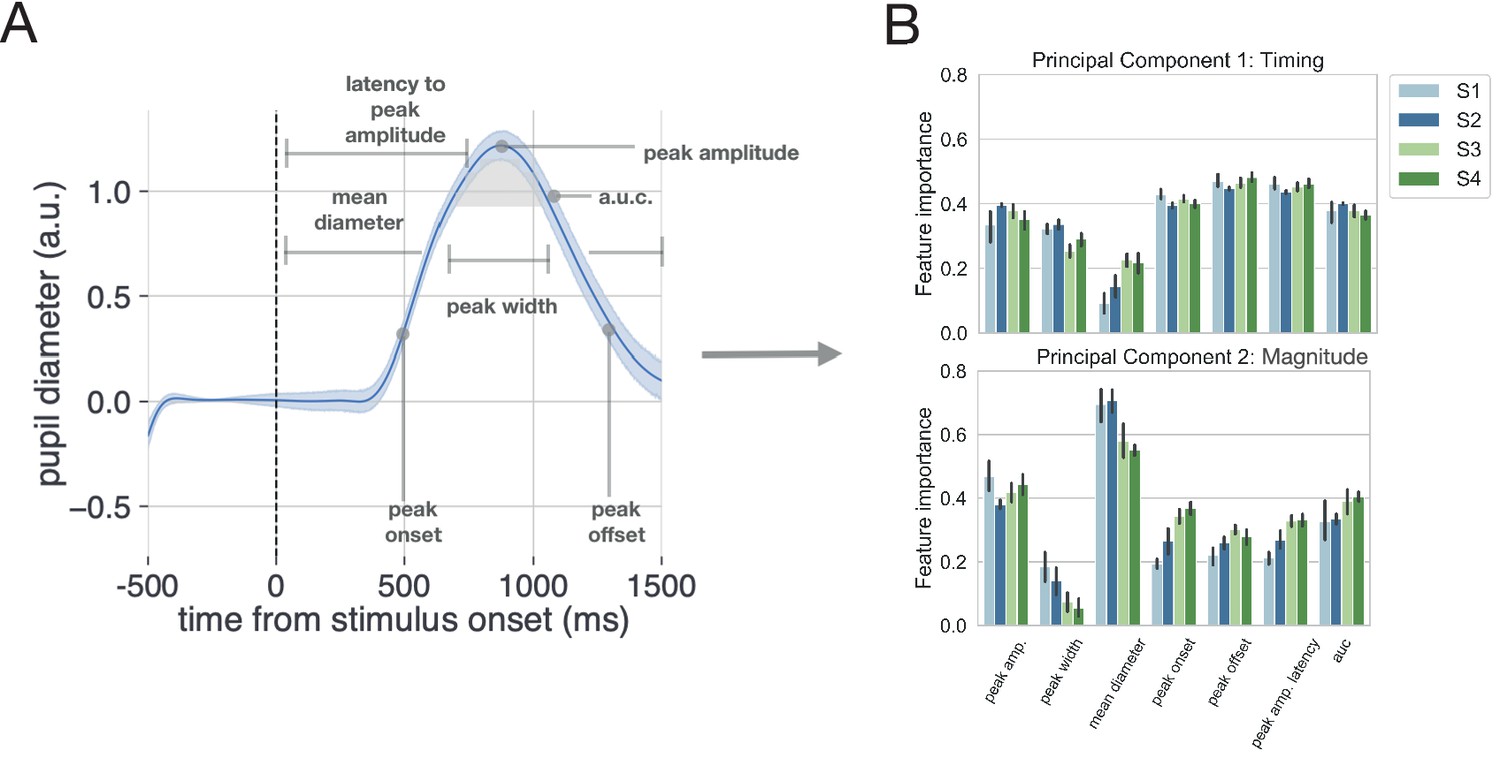
Method for analyzing pupil data.

(A) The evoked pupillary response was characterized according to seven metrics. (B) These pupillary features were submitted to a principal component analysis. The contribution of each feature to the variance explained for the first two components is plotted for each subject. Note that we also conducted a supplementary analysis of the task-evoked pupillary response using a more conventional method with similar results.

Figure 10

Download asset Open asset

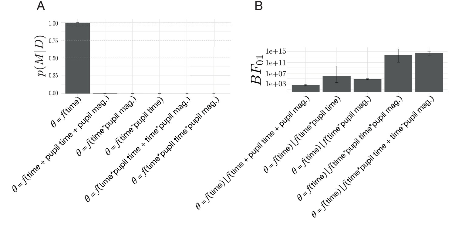
Model comparisons for the effect of change-point-evoked pupillary dynamics on the relationship between drift rate and boundary height ( $θ$ ).

(A) The posterior probability for models testing for an effect of pupillary dynamics on $θ$ . (B) The Bayes Factor for the evoked response model relative to the alternative models specifying an effect of pupillary dynamics on the evoked response, $θ$ . Note that time refers to time relative to the onset of a change point. All models specifying an interaction also include main effects.

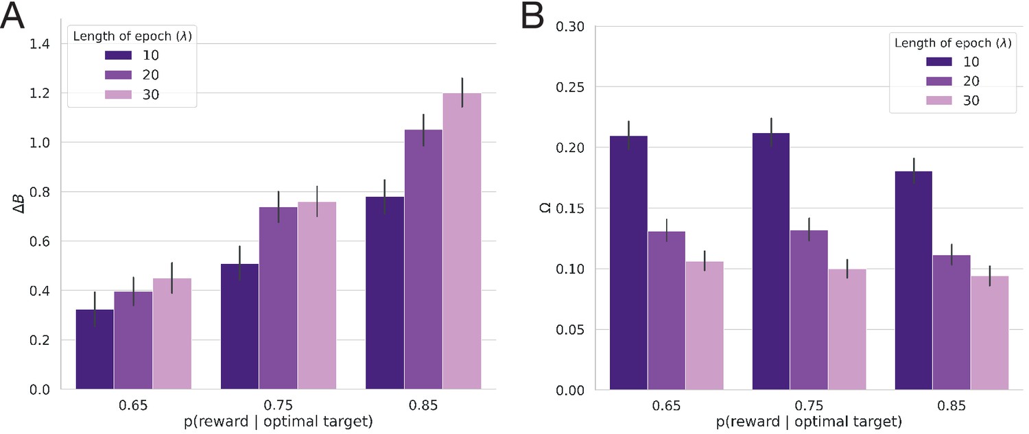
Appendix 1—figure 1

Download asset Open asset

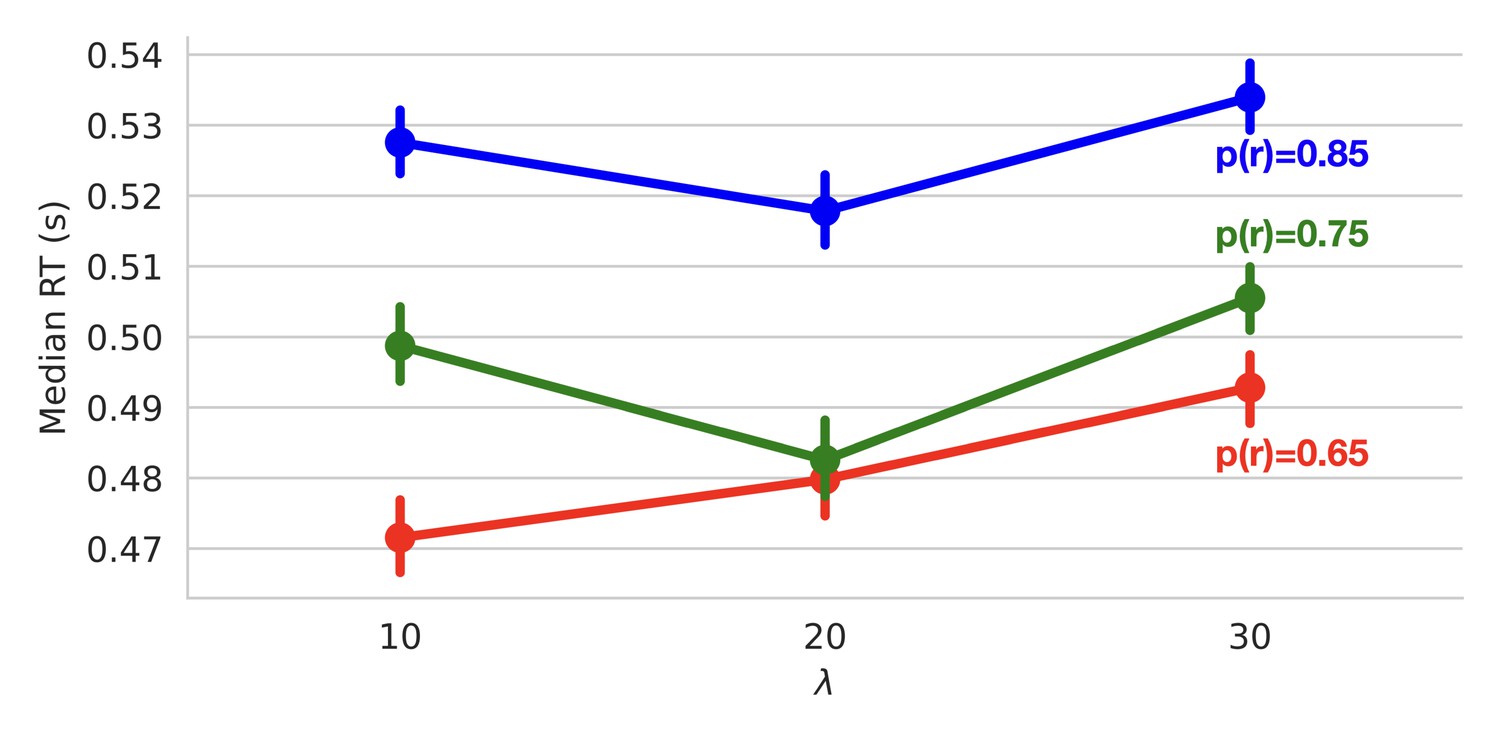
Reaction times.

Median reaction times as a function of volatility (epoch length; $λ$ ) and conflict (probability of reward; $p (r)$ ).

Appendix 1—figure 2

Download asset Open asset

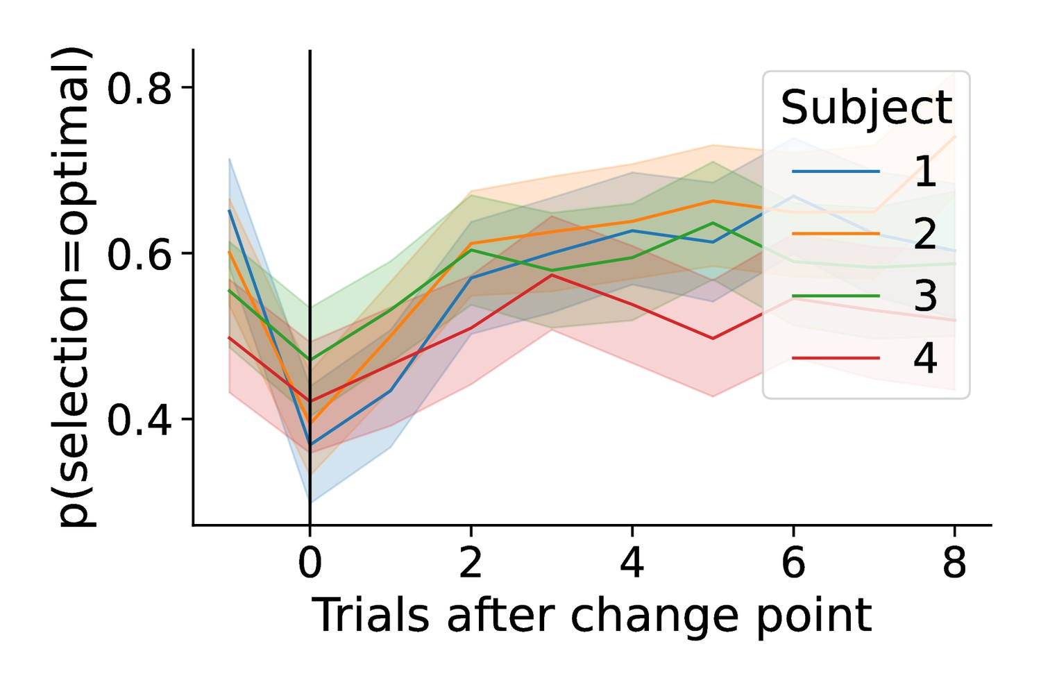
Change-point-evoked accuracy.

Change-point-evoked accuracy by subject.

Appendix 1—figure 3

Download asset Open asset

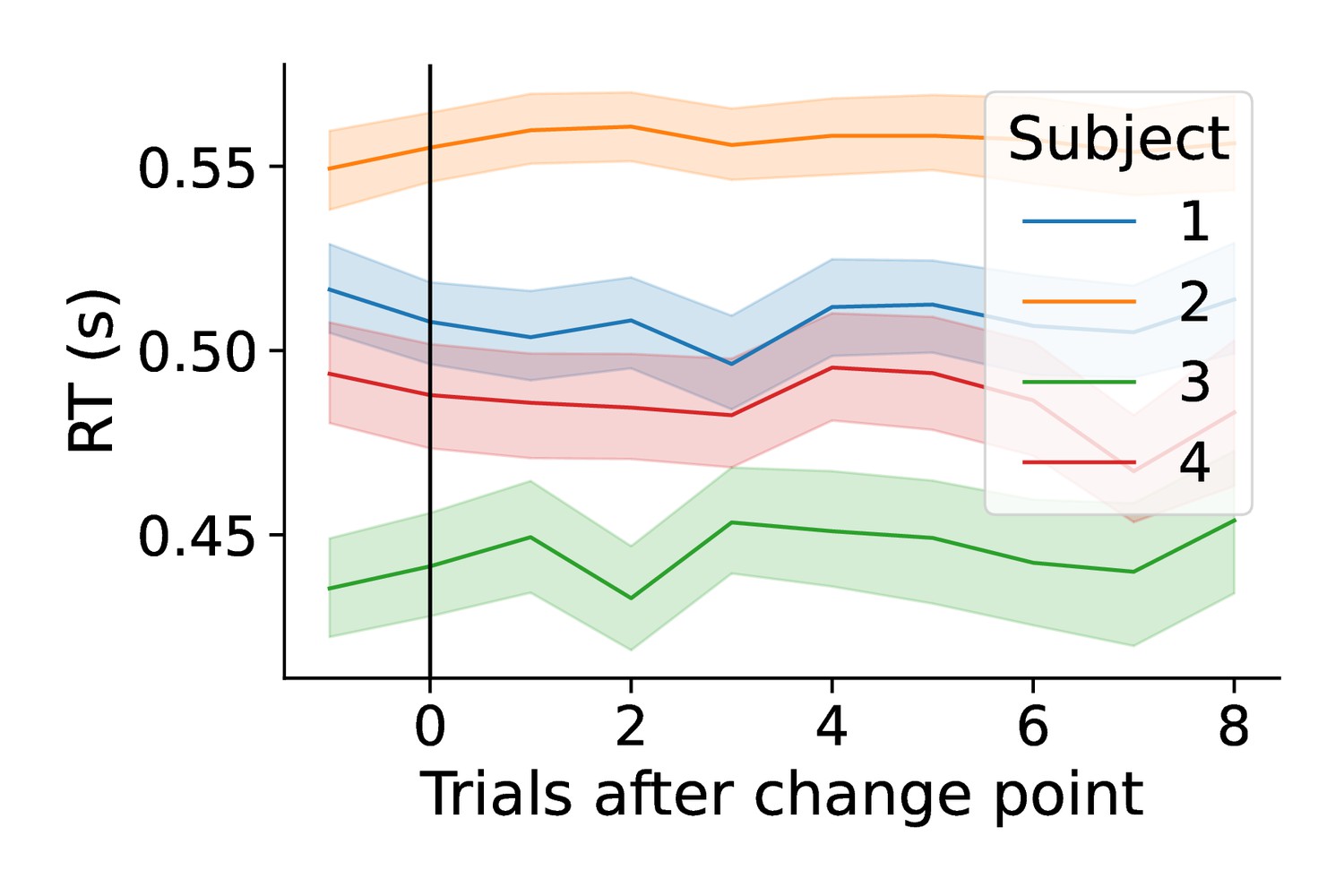
Change-point evoked reaction times.

Change-point-evoked reaction times by subject.

Appendix 1—figure 4

Download asset Open asset

Ideal observer estimates for Experiment 2.

(A) The average belief in the value of the optimal target ( $Δ B$ ) as a function of the probability of reward (conflict) and the average period of stability for the optimal choice ( $λ$ ; volatility). (B) Average change point probability ( $Ω$ ) as a function of conflict and volatility.

Appendix 1—figure 5

Download asset Open asset

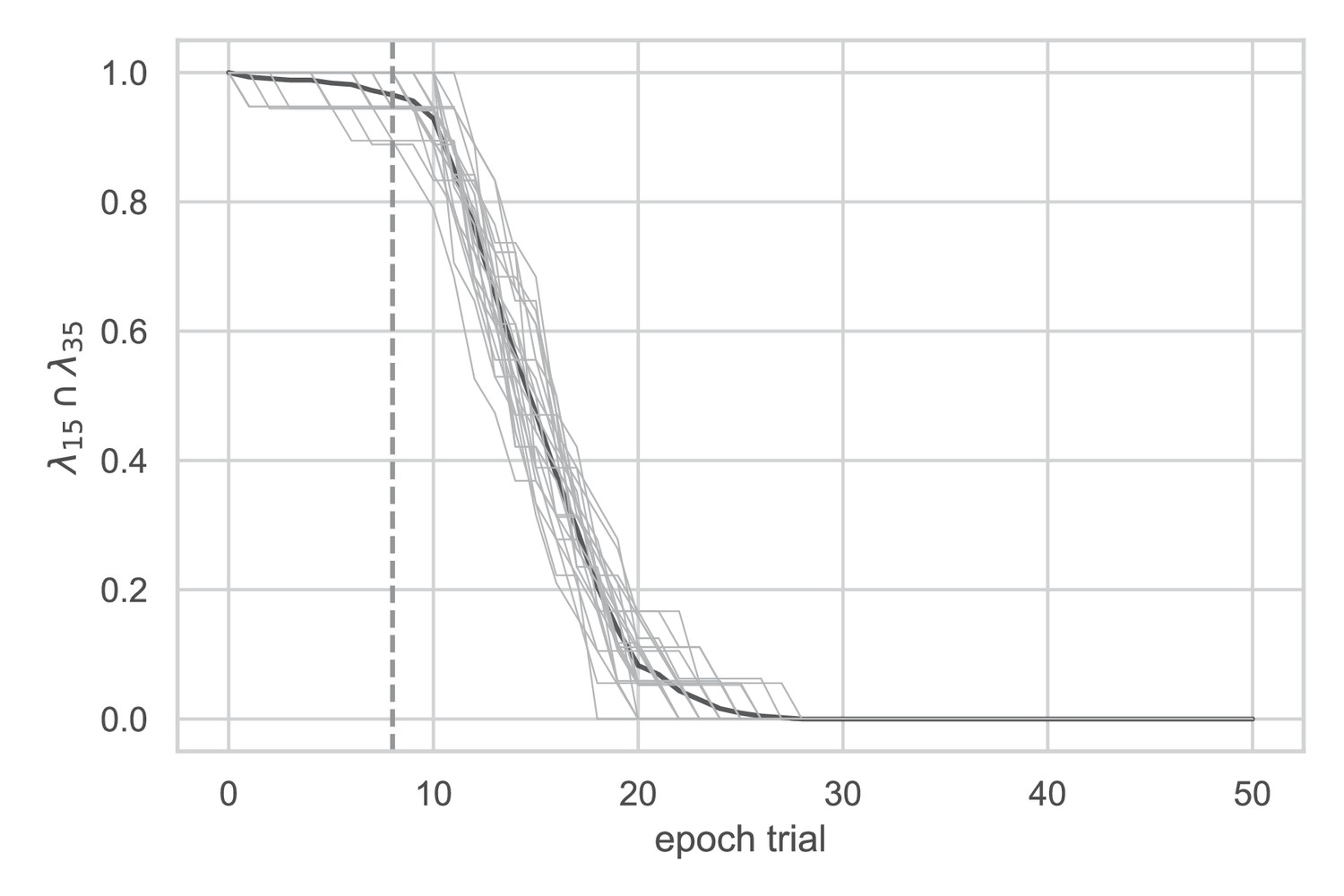
Initial window selection.

Analysis conducted on data from Experiment 1 to determine the timescale of the response that maximized the intersection between high volatility ( $λ = 15$ ) and low volatility ( $λ = 35$ ) data. The bolded line represents the mean and the gray lines represent individual subjects. The dotted line indicates the initial window of nine trials used.

Appendix 1—figure 6

Download asset Open asset

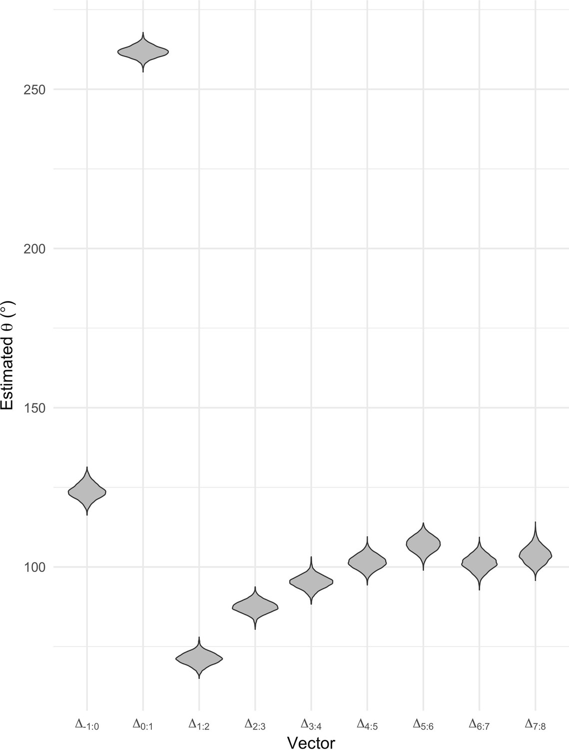
Stability analysis.

Analysis conducted on Experiment 1 to determine the timescale of the response to consider for Experiment 2. The estimated angle is plotted as a function of time within an epoch (estimate from circular regression).

Appendix 1—figure 7

Download asset Open asset

Quantification of stability.

Probability that sequential posterior distributions for $β_{Δ t}$ have equal means.

Appendix 1—figure 8

Download asset Open asset

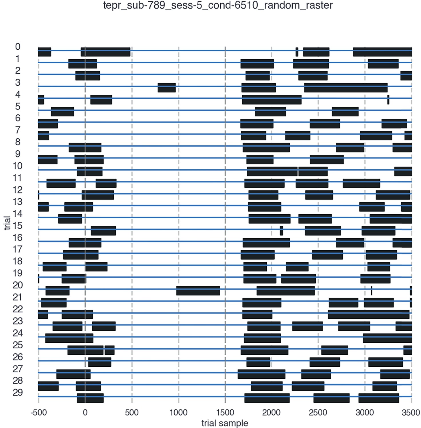
Blink timing.

Blink timing for a sample participant. For visibility, thirty trials were selected at random. The onset of the trial is marked as time 0 and the trial ends at 1500ms. Blinks are marked in black. Blink timing plots are available for all subjects and all conditions in the GitHub repository for this publication.

Appendix 1—figure 9

Download asset Open asset

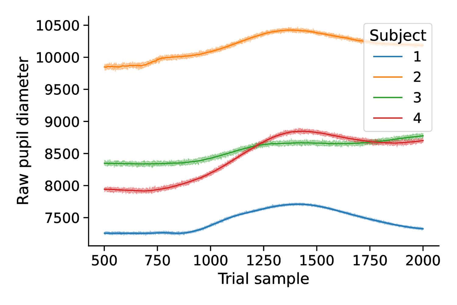
Raw pupil diameter.

Mean time course of pupil diameter by subject.

Appendix 1—figure 10

Download asset Open asset

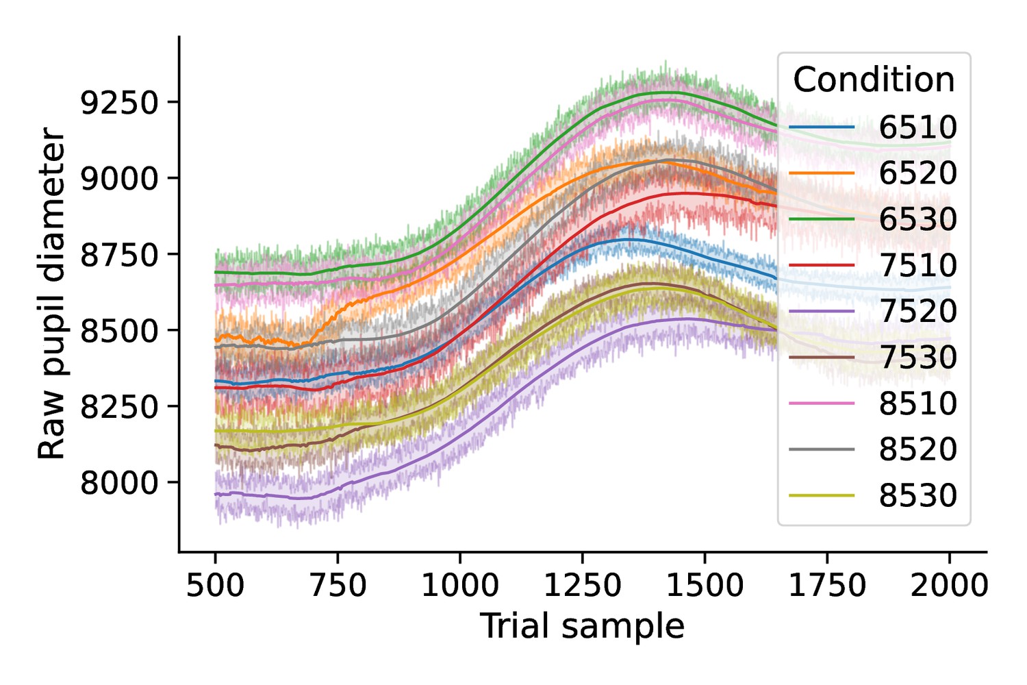
Evoked pupil diameter by condition.

Mean time course of pupil diameter by condition.

Appendix 1—figure 11

Download asset Open asset

First temporal derivative of pupil diameter.

Mean time course of derivative of pupil diameter by subject.

Appendix 1—figure 12

Download asset Open asset

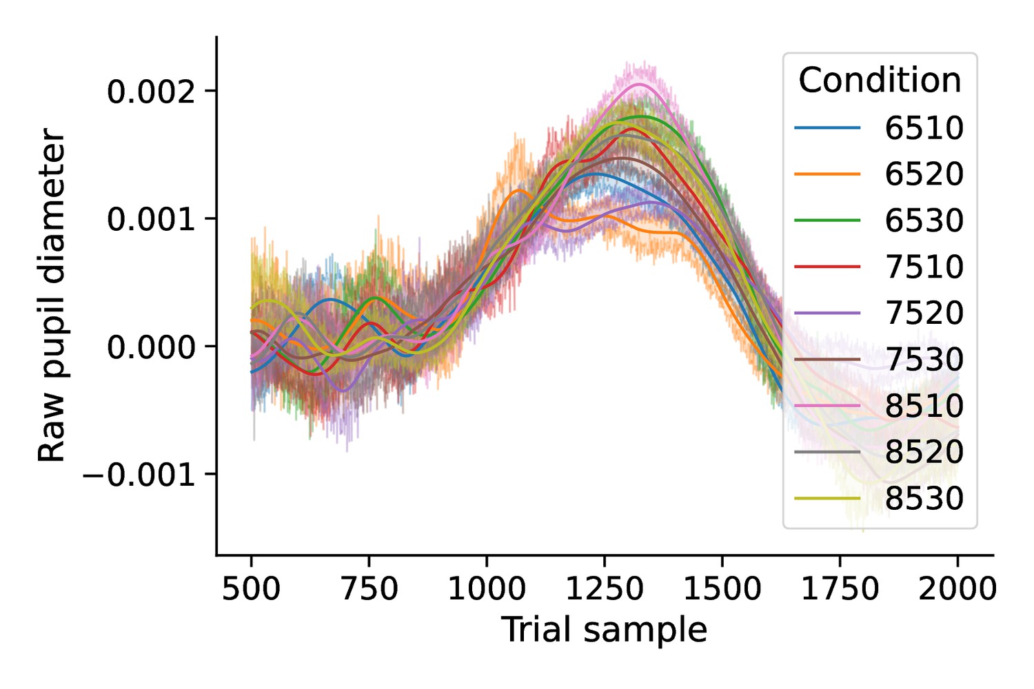
Derivative of evoked pupil diameter by condition.

Mean time course of derivative of pupil diameter by condition.

Appendix 1—figure 13

Download asset Open asset

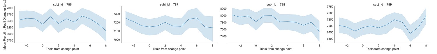
Prestimulus pupillary response.

Mean prestimulus pupillary response by subject.

Tables

Table 1

Model comparison for Experiments 1 and 2.

Roman numerals refer to a given model, as defined by the mapping between the ideal observer estimates and decision parameters in the first two columns. The left panel shows the deviance information criterion (DIC) scores for the set of models considered during the model selection procedure for Experiment 1. The right panel shows the DIC scores for the equivalent model selection analysis for Experiment 2, with a model estimated for each of four subjects. Values shown represent the mean and standard deviation computed over subjects. Note that the raw DIC values for each of the subjects in Experiment 2 are included in Appendix 3—table 1. The column labeled DIC gives the raw DIC score, $Δ {DIC}_{n u l l}$ lists the change in model fit from an intercept-only model (the null-adjusted fit), and $Δ {DIC}_{b e s t}$ provides the change in null-adjusted model fit from the best-fitting model. The best performing model is denoted by an asterisk, with equivocal best cases marked by a tilde.

Experiment 1
	$Δ B$	$Ω$	DIC	$Δ {DIC}_{null}$	$Δ D I C_{b e s t}$
*I	$v$	$a$	–18643.9	–2698.0	0.0
II	$a$	$v$	–16265.6	–319.7	2378.3
III	–	$v$	–16180.5	–234.7	2463.3
IV	$v$	–	–18630.8	–2684.9	13.1
V	–	$a$	–15949.20	–3.4	2694.7
VI	$a$	–	–16032.8	–87.0	2611.1
VII	–	–	–15945.8	0.0	2698.0
Experiment 2
	$Δ B$	$Ω$	$Δ {DIC}_{null}$	$Δ {DIC}_{best}$
*∼I	$v$	$a$	–90.3 ± 71.7	1.0 ± 0.8
II	$a$	$v$	–7.6 ± 13.1	83.8 ± 60.5
III	–	$v$	–8.5 ± 13.1	82.9 ± 61.4
*∼IV	$v$	–	–90.8 ± 71.0	0.5 ± 1.1
V	–	$a$	0.3 ± 2.5	91.6 ± 70.6
VI	$a$	–	0.95 ± 1.4	92.3 ± 70.9
VII	–	–	0 ± 0	91.3 ± 71.5

Appendix 2—table 1

Power analysis for Experiment 1.

The results of the model comparison analysis using simulated data. Roman numerals refer to a given model, as defined by the mapping between the ideal observer estimates and decision parameters in the first two columns. The column labeled DIC gives the raw DIC score, $Δ {DIC}_{n u l l}$ lists the change in model fit from an intercept-only model (the null-adjusted fit), and $Δ {DIC}_{b e s t}$ provides the change in null-adjusted model fit from the best-fitting model. The last row represents the null, intercept-only regression model. The best performing model is denoted by an asterisk.

	$B$	$Ω$	DIC	$Δ {DIC}_{null}$	$Δ {DIC}_{best}$
I*	$v$	$a$	–101886.4	–15477.5	0.0
II	$a$	$v$	–87486.7	–1077.8	14399.7
III	–	$v$	–87373.9	–965.0	14512.5
IV	$v$	–	–97634.70	–11225.8	4251.70
V	–	$a$	–90577.3	–4168.40	11309.00
VI	$a$	–	–86525.7	–116.70	15360.7
VII	–	–	–86408.9	0.0	15477.5

Appendix 3—table 1

Raw model selection results for Experiment 2.

The raw results of the model comparison analysis conducted depicted in Table 1 for Experiment 2. Roman numerals refer to a given model, as defined by the mapping between the ideal observer estimates and decision parameters in the first two columns. The column labeled DIC gives the raw DIC score, $Δ {DIC}_{n u l l}$ lists the change in model fit from an intercept-only model (the null-adjusted fit), and $Δ {DIC}_{b e s t}$ provides the change in null-adjusted model fit from the best-fitting model. The last row for each subject represents the null, intercept-only regression model. Equivocal winning models marked with an asterisk and a tilde.

Subject	$Δ B$	$Ω$	$D I C$	$Δ D I C_{n u l l}$	$Δ D I C_{b e s t}$
1	v	a	5286.0	–156.1	1.8 * $s i m$
1	a	v	5430.2	–11.9	146.0
1	-	v	5431.3	–10.8	147.1
1	v	-	5284.1	–157.9	0.0 * $s i m$
1	-	a	5444.0	2.0	159.9
1	a	-	5441.1	–0.9	157.0
1	-	-	5442.0	0.0	157.9
2	v	a	5162.9	–144.1	0.0 * $s i m$
2	a	v	5283.0	–24.1	120.0
2	-	v	5281.0	–26.1	118.0
2	v	-	5165.1	–142.0	2.1 * $s i m$
2	-	a	5303.7	–3.4	140.8
2	a	-	5309.2	2.1	146.2
2	-	-	5307.1	0.0	144.1
3	v	a	3034.8	–53.4	0.7 * $s i m$
3	a	v	3090.1	1.9	56.0
3	-	v	3089.5	1.2	55.4
3	v	-	3034.1	–54.1	0.0 * $s i m$
3	-	a	3089.2	0.9	55.1
3	a	-	3088.8	0.6	54.7
3	-	-	3088.2	0.0	54.1
4	v	a	5438.9	–7.7	1.4 * $s i m$
4	a	v	5450.5	3.8	13.0
4	-	v	5448.5	1.8	11.0
4	v	-	5437.5	–9.1	0.0 * $s i m$
4	-	a	5448.2	1.6	10.7
4	a	-	5448.7	2.0	11.2
4	-	-	5446.7	0.0	9.1