Genetic architecture of 11 organ traits derived from abdominal MRI using deep learning
- Calico Life Sciences LLC, United States
- Research Centre for Optimal Health, School of Life Sciences, University of Westminster, United Kingdom
Figures
Figure 1 with 2 supplements
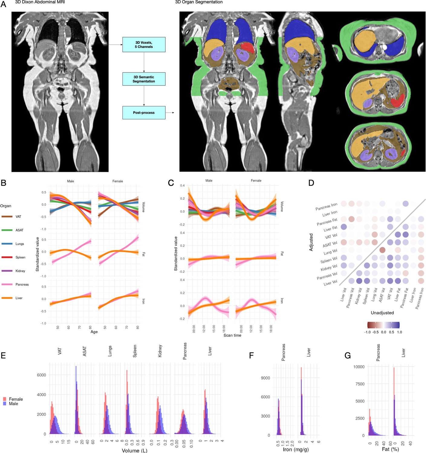
Visualisation of studied IDPs.
(A) Example Dixon image before and after automated segmentation of ASAT, VAT, liver, lungs, left and right kidneys, and spleen. (B) Relationship between IDPs and age and sex within the UKBB. Each trait is standardised within sex, so that the y axis represents standard deviations, after adjustment for imaging centre and date. The trend is smoothed using a generalised additive model with smoothing splines for visualisation purposes. (C) Relationship between IDPs and scan time and sex within the UKBB. Each trait is standardised within sex, so that the y axis represents standard deviations, after adjustment for imaging centre and date. The trend is smoothed using a generalised additive model with smoothing splines for visualisation purposes. (D) Correlation between IDPs. Lower right triangle: Unadjusted correlation (except for imaging centre and date). Upper left triangle: Correlation after adjustment for age, sex, height, and BMI. (E-G) Histograms showing the distribution of the eleven IDPs in this study.
Figure 1—figure supplement 1
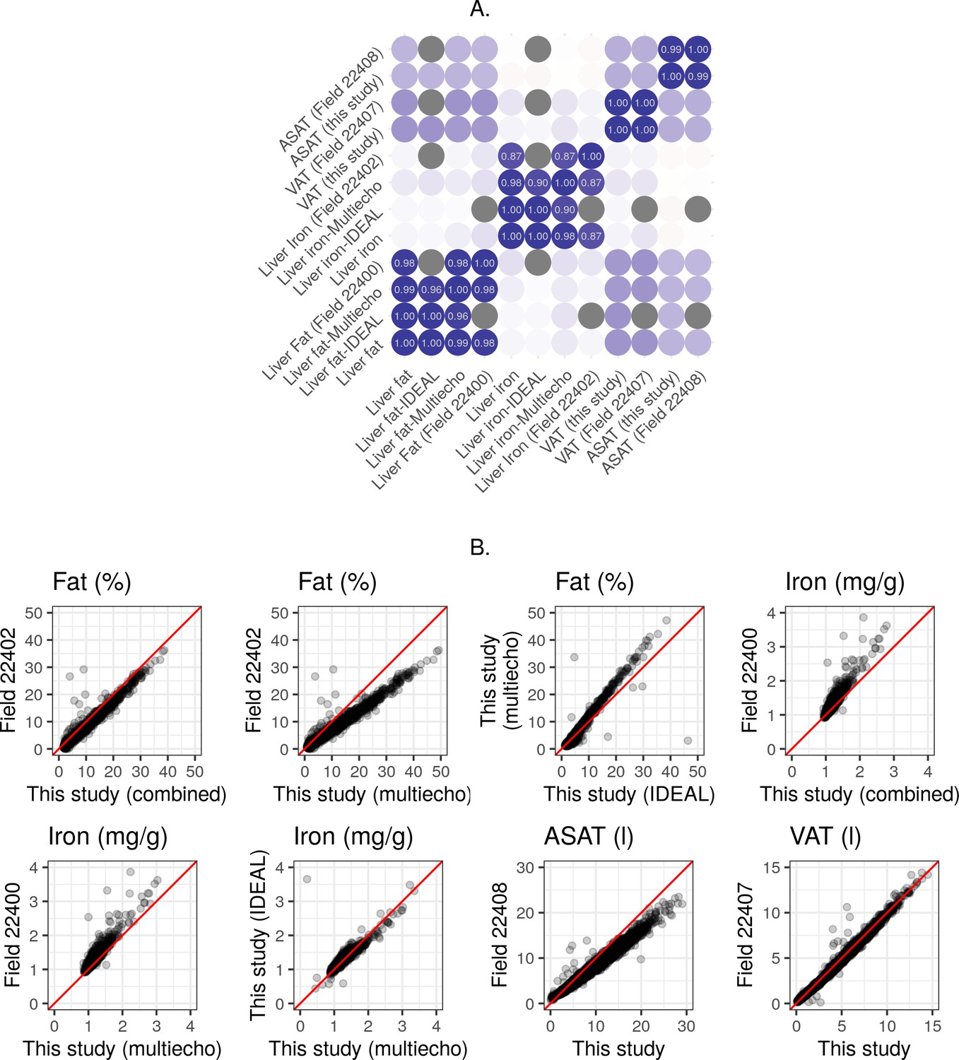
Correlation between multiple measurements of fat, iron and volume.
(A) Correlation between multiple measurements of liver fat, liver iron, ASAT volume, and VAT volume in the UK Biobank. (B) Scatter plots showing the relationship between multiple measurements of liver fat, liver iron, ASAT volume, and VAT volume in the UK Biobank. ‘Combined’ refers to a combined IDEAL/multiecho measurement as described in the ‘multiecho pipeline’ section of the supplementary information.
Figure 1—figure supplement 2
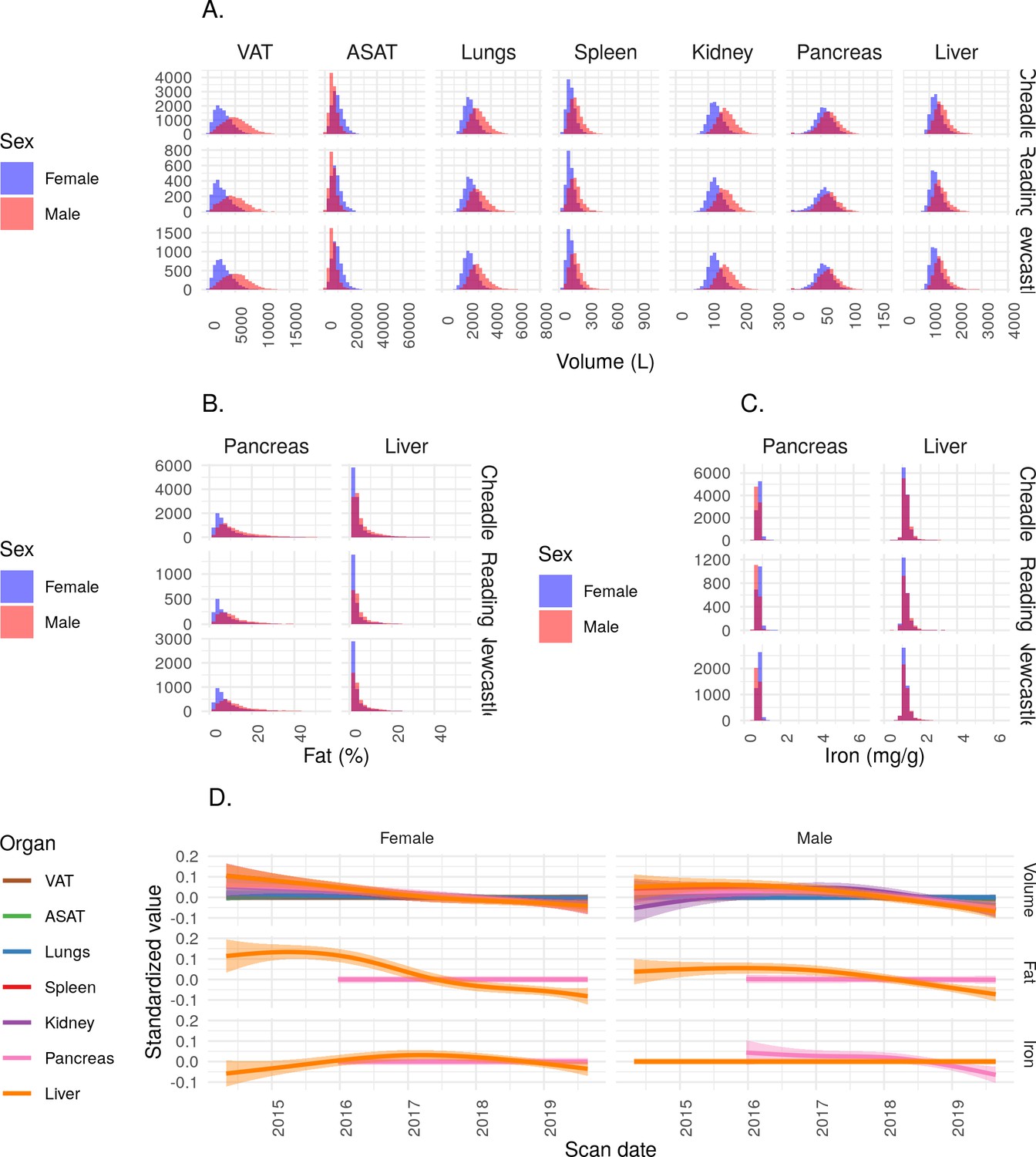
IDPs plotted across imaging centre and across scan date.
(A) Organ volume IDPs, split by imaging centre. (B) Fat IDPs, split by imaging centre. (C) Iron IDPs, split by imaging centre. (D) Relationship between scan date and IDPs.
Figure 2 with 5 supplements

Disease phenome-wide association study across all IDPs and 754 disease codes (PheCodes).
The x-axis gives the effect size per standard deviation, and the y-axis -log10(p-value). The top three associations for each phenotype are labelled. Horizontal lines at disease phenome-wide significance (dotted line, p=6.63e-05) and study-wide significance (dashed line, p=6.03e-06) after Bonferroni correction. Note that the PheCodes are not exclusive and have a hierarchical structure (for example, T1D and T2D are subtypes of Diabetes), so some diseases appear more than once in these plots. LL: Leukocytic leukaemia. CLL: Chronic leukocytic leakaemia. T1D: Type 1 diabetes. T2D: Type 2 diabetes. CKD: Chronic kidney disease.
-
Figure 2—source data 1
Source data for Figure 2 and Figure 2—figure supplement 1–5, phenome-wide association study across all IDPs.
- https://cdn.elifesciences.org/articles/65554/elife-65554-fig2-data1-v1.zip
Figure 2—figure supplement 1
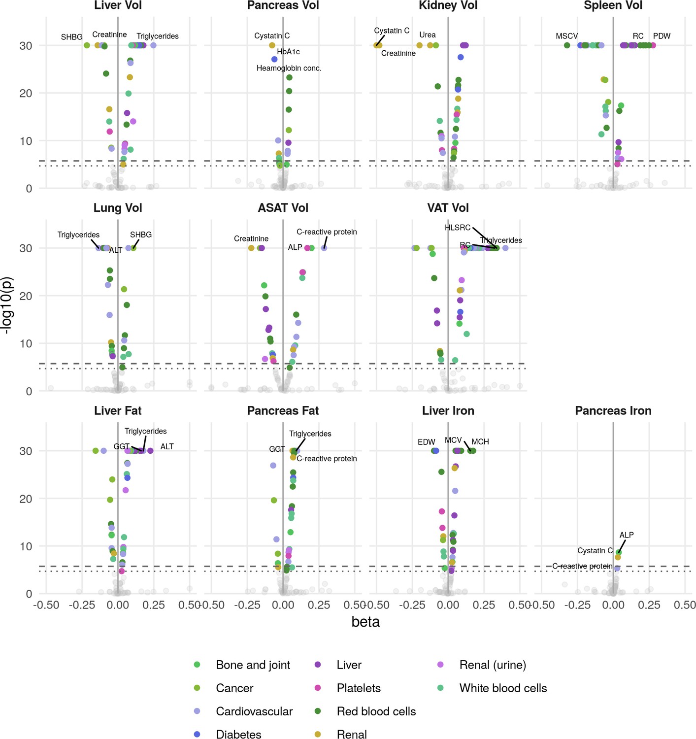
Phenome-wide associations across all IDPs and 83 biomarkers.
The x-axis gives the effect size per standard deviation, and the y-axis -log10(p-value). The top three associations for each phenotype are labelled. Horizontal lines at phenome-wide significance (dotted line, p=2.7e-05) and study-wide significance (dashed line, p=2.48e-06) after Bonferroni correction for the total number of measures. SHBG: Sex hormone binding globulin. MSCV: Mean sphered cell volume. MCH: Mean corpuscular haemoglobin. RC: Reticulocyte count. PDW: Platelet distribution width. ALT: alanine transaminase. ALP: Alkaline phosphatase. HLSRC: High light scatter reticulocyte count. GGT: Gamma glutamyl transferase.
Figure 2—figure supplement 2
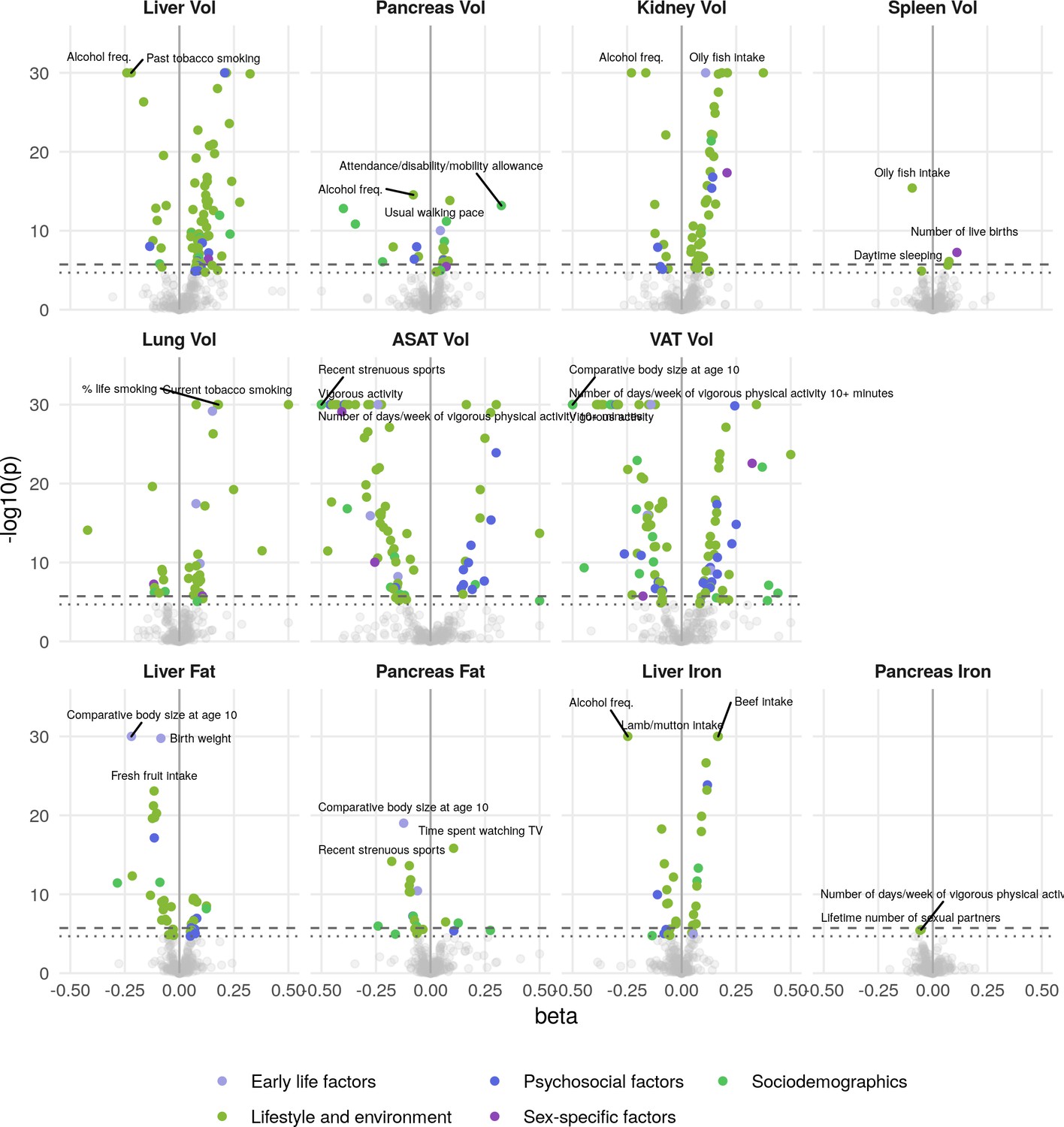
Phenome-wide associations across all IDPs and 199 lifestyle and history traits.
The x-axis gives the effect size per standard deviation, and the y-axis -log10(p-value). The top three associations for each phenotype are labelled. Horizontal lines at phenome-wide significance (dotted line, p=2.7e-05) and study-wide significance (dashed line, p=2.48e-06) after Bonferroni correction for the total number of measures.
Figure 2—figure supplement 3
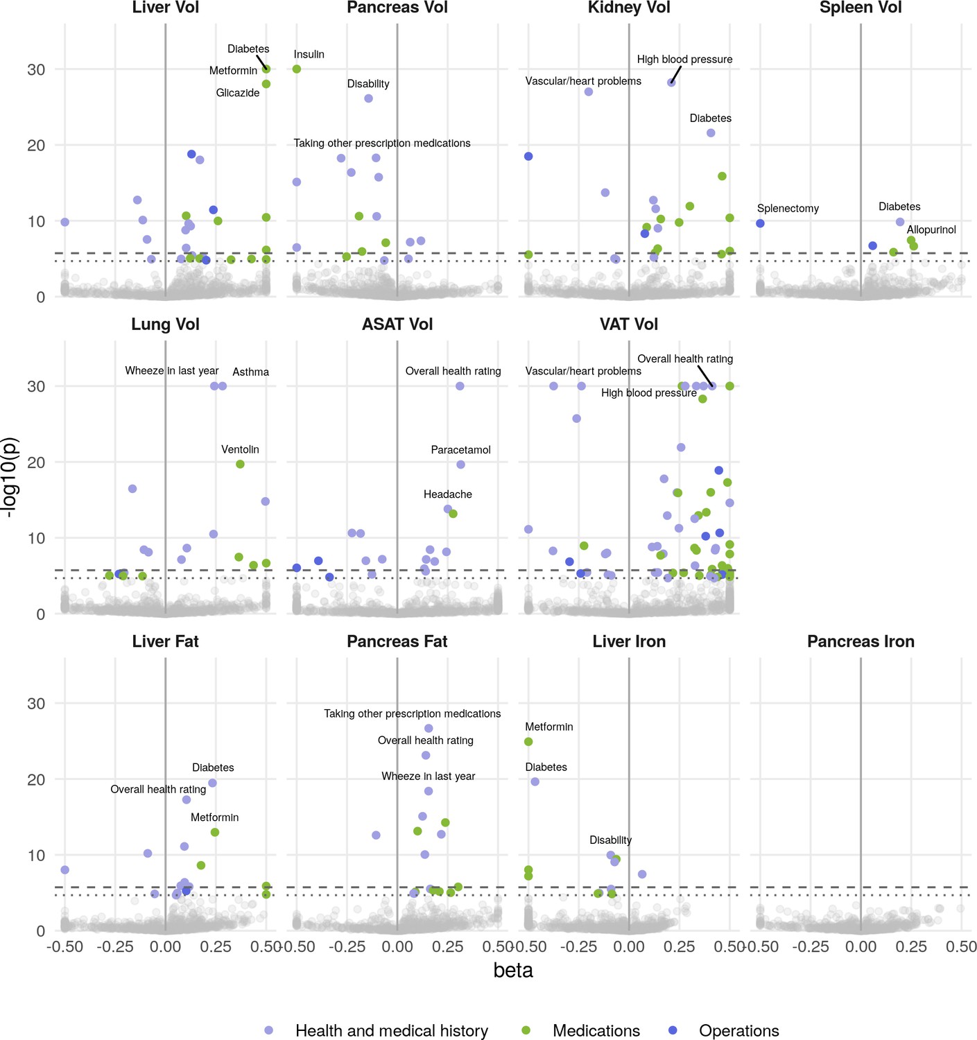
Phenome-wide associations across all IDPs and 770 medical history traits.
The x-axis gives the effect size per standard deviation, and the y-axis -log10(p-value). The top three associations for each phenotype are labelled. Horizontal lines at phenome-wide significance (dotted line, p=2.7e-05) and study-wide significance (dashed line, p=2.48e-06) after Bonferroni correction for the total number of measures.
Figure 2—figure supplement 4
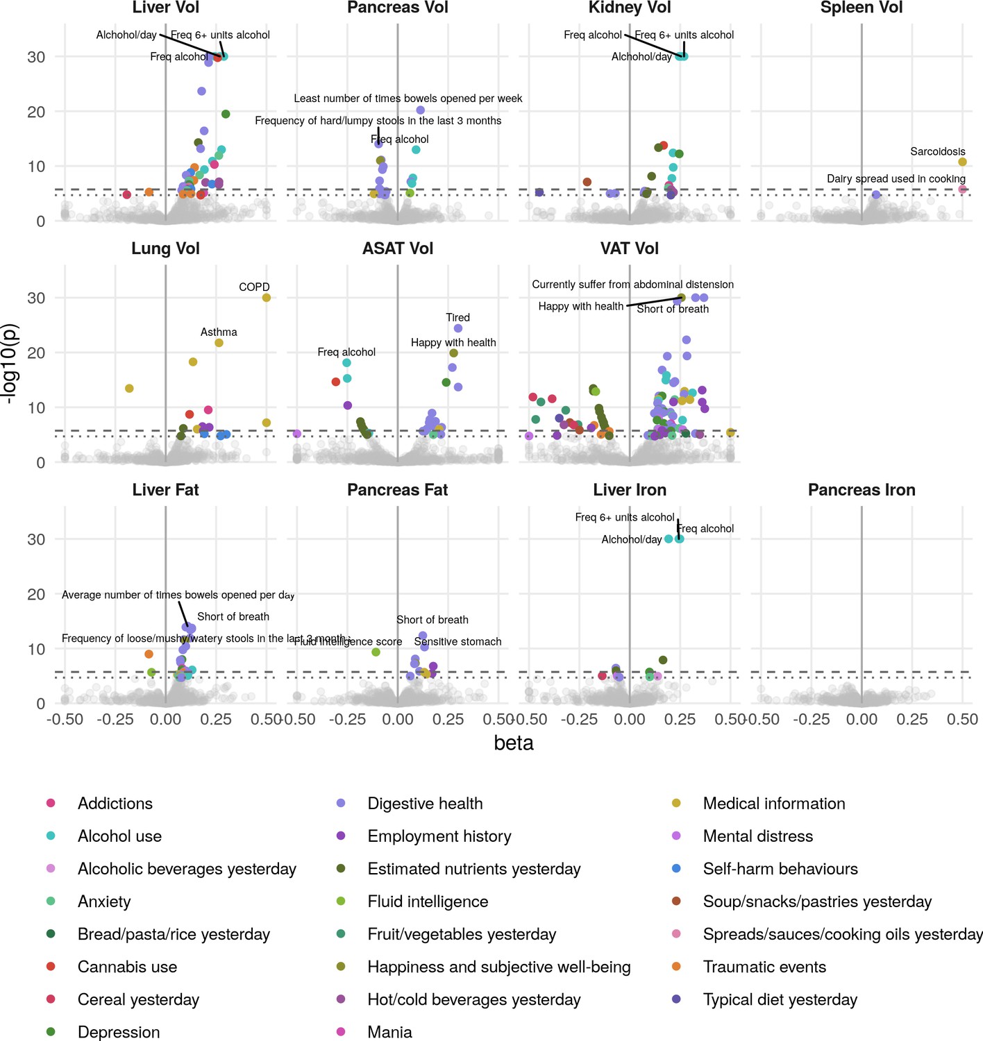
Phenome-wide associations across all IDPs and 444 traits measured in online follow-up.
The x-axis gives the effect size per standard deviation, and the y-axis -log10(p-value). The top three associations for each phenotype are labelled. Horizontal lines at phenome-wide significance (dotted line, p=2.7e-05) and study-wide significance (dashed line, p=2.48e-06) after Bonferroni correction for the total number of measures.
Figure 2—figure supplement 5
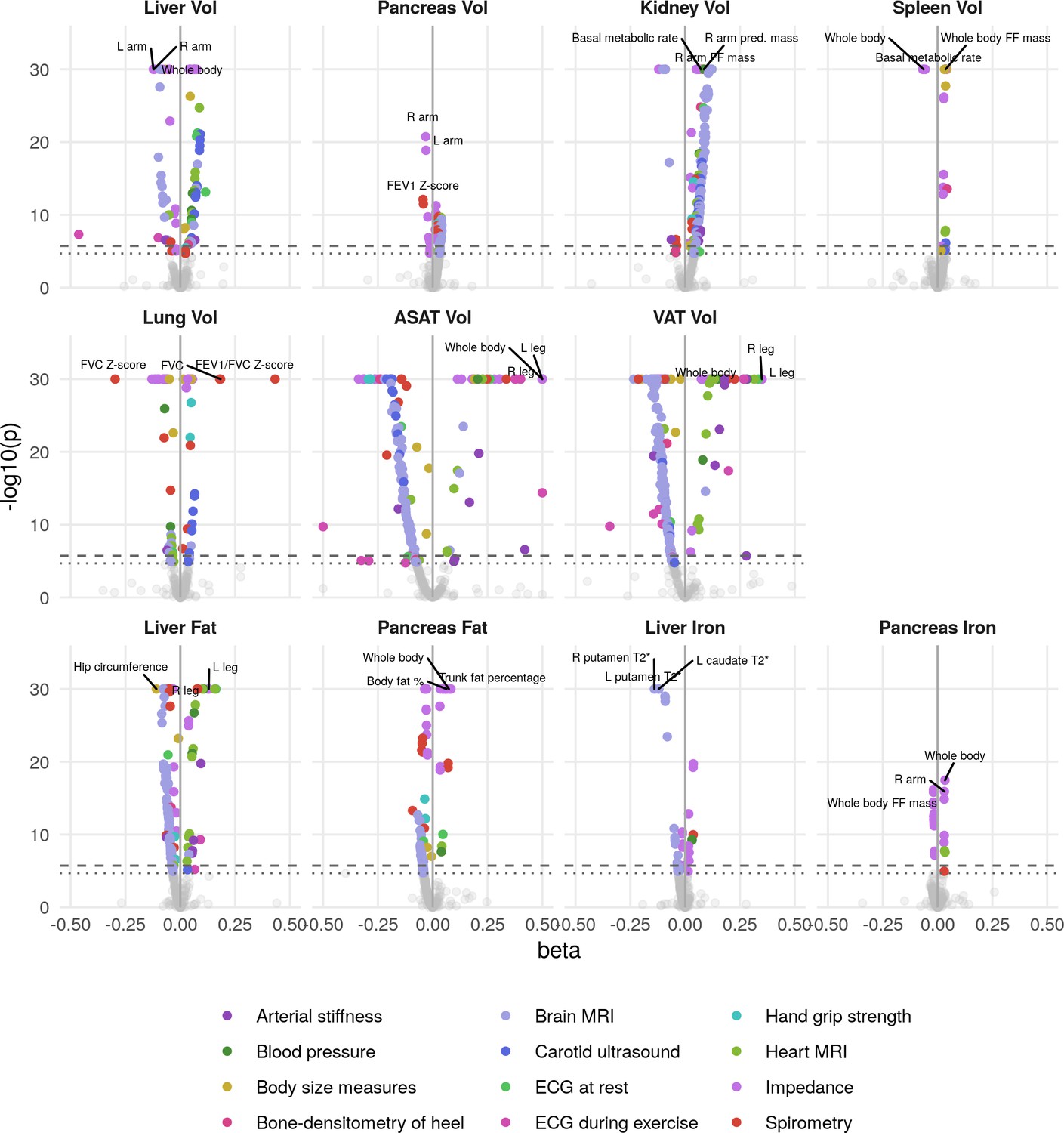
Phenome-wide associations across all IDPs and 335 physical measures.
The x-axis gives the effect size per standard deviation, and the y-axis -log10(p-value). The top three associations for each phenotype are labelled. Horizontal lines at phenome-wide significance (dotted line, p=2.7e-05) and study-wide significance (dashed line, p=2.48e-06) after Bonferroni correction for the total number of measures. FVC forced vital capacity. FEV1 Forced expiratory volume in 1 s. FF fat-free.
Figure 3 with 6 supplements

Genetic architecture of all IDPs.
(A) Heritability (point estimate and 95% confidence interval) for each IDP estimated using the BOLT-REML model. Y-axis: Adjusted for height and BMI. X-axis: Not adjusted for height and BMI. The three panels show volumes, fat, and iron respectively. (B) Genetic correlation between IDPs estimated using bivariate LD score regression. The size of the points is given by -log10(p), where p is the p-value of the genetic correlation between the traits. Upper left triangle: Adjusted for height and BMI. Lower right triangle: Not adjusted for height and BMI. (C) Manhattan plots showing genome-wide signals for all IDPs for volume (top panel), fat (middle panel), and iron concentration (lower panel). Horizontal lines at 5e-8 (blue dashed line, genome-wide significant association for a single trait) and 4.5e-9 (red dashed line, study-wide significant association). P-values are capped at 10e-50 for ease of display. The genes with closest transcription start site are labelled.
Figure 3—figure supplement 1
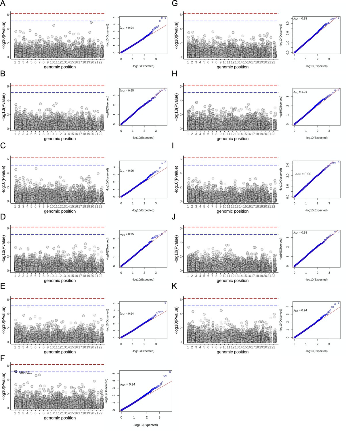
Rare association studies in the subcohort with both exome sequence data and imaging-derived quantitative phenotypes.
Left: Manhattan plot shows the association between each gene organised by genomic coordinates. Right: QQ-plot showing calibration of SKAT-O test statistics. λGC: Genomic control parameter for each trait. Blue dashed line indicates Bonferroni significance threshold genome-wide (p=7.4e-06). Red dashed line indicates overall study significance threshold (p=6.7e-07). (A) Volume of visceral fat (n = 11,069 samples) .(B) Volume of spleen (n = 11,134). (C) Volume of the lungs (n = 11,134). (D) Liver volume (n = 11,134). (E) Kidney volume (n = 11,134). (F) Abdominal subcutaneous fat (n = 11,134). One gene achieved genome-wide significance but not study wide significance (RRNAD1: pSKAT-O = 6.5e-06; betaburden = −0.08). (G) Pancreas volume (n = 11,093) (H) pancreas iron level (n = 5,525) (I) liver iron (n = 11,069) (J) pancreatic fat (n = 5525) (K) liver fat (n = 11,069).
Figure 3—figure supplement 2
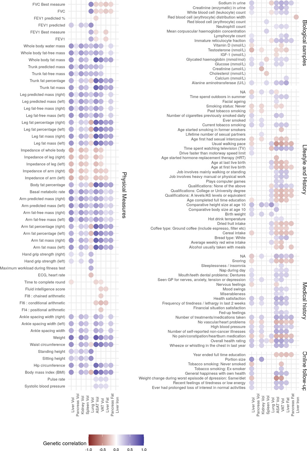
Genetic correlation between IDPs and complex traits.
Only IDPs and traits with statistically significant genetic correlation (p<1.61e-05 after Bonferroni correction for multiple testing) are shown.
Figure 3—figure supplement 3
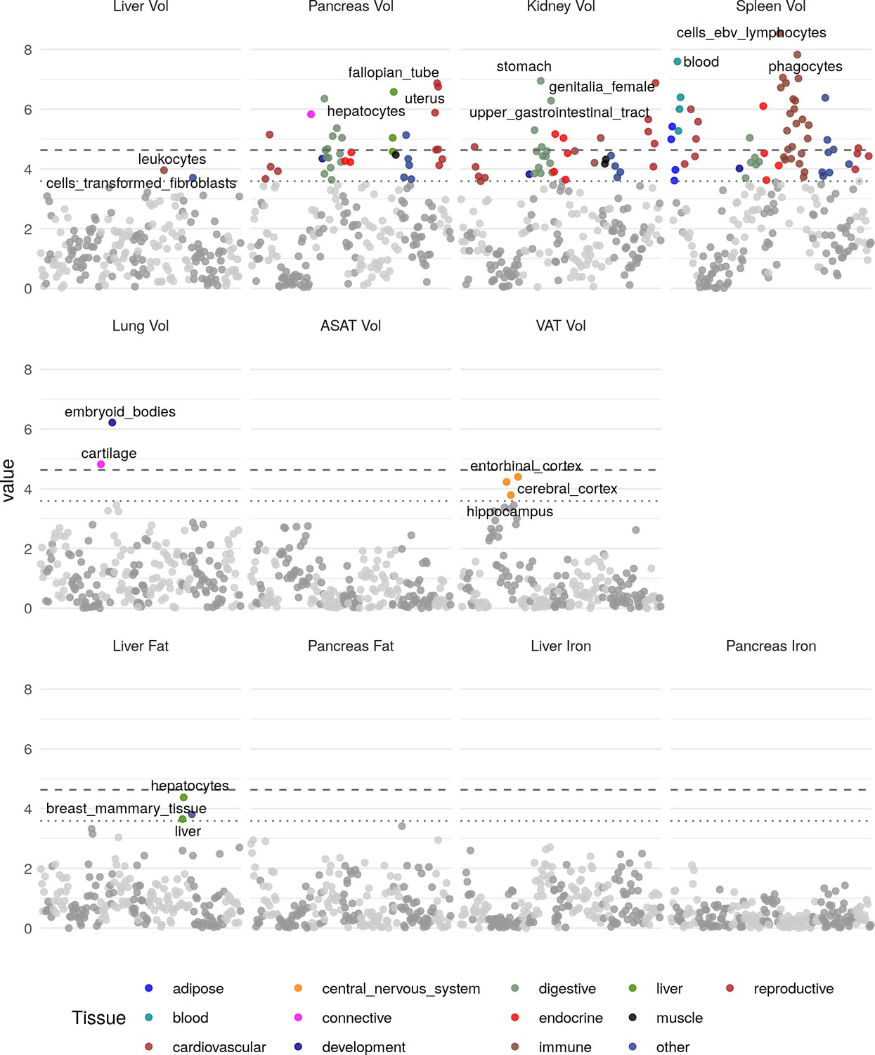
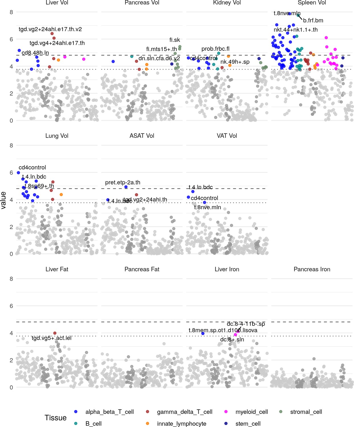
Heritability enrichment in tissues and cell types for annotations based on gene expression (see Materials and methods).
The top three enrichments for each phenotype passing a trait-wide significance threshold are labelled. Horizontal lines and trait-wide (dotted line) and study-wide (dashed line) significance after Bonferroni correction.
Figure 3—figure supplement 4
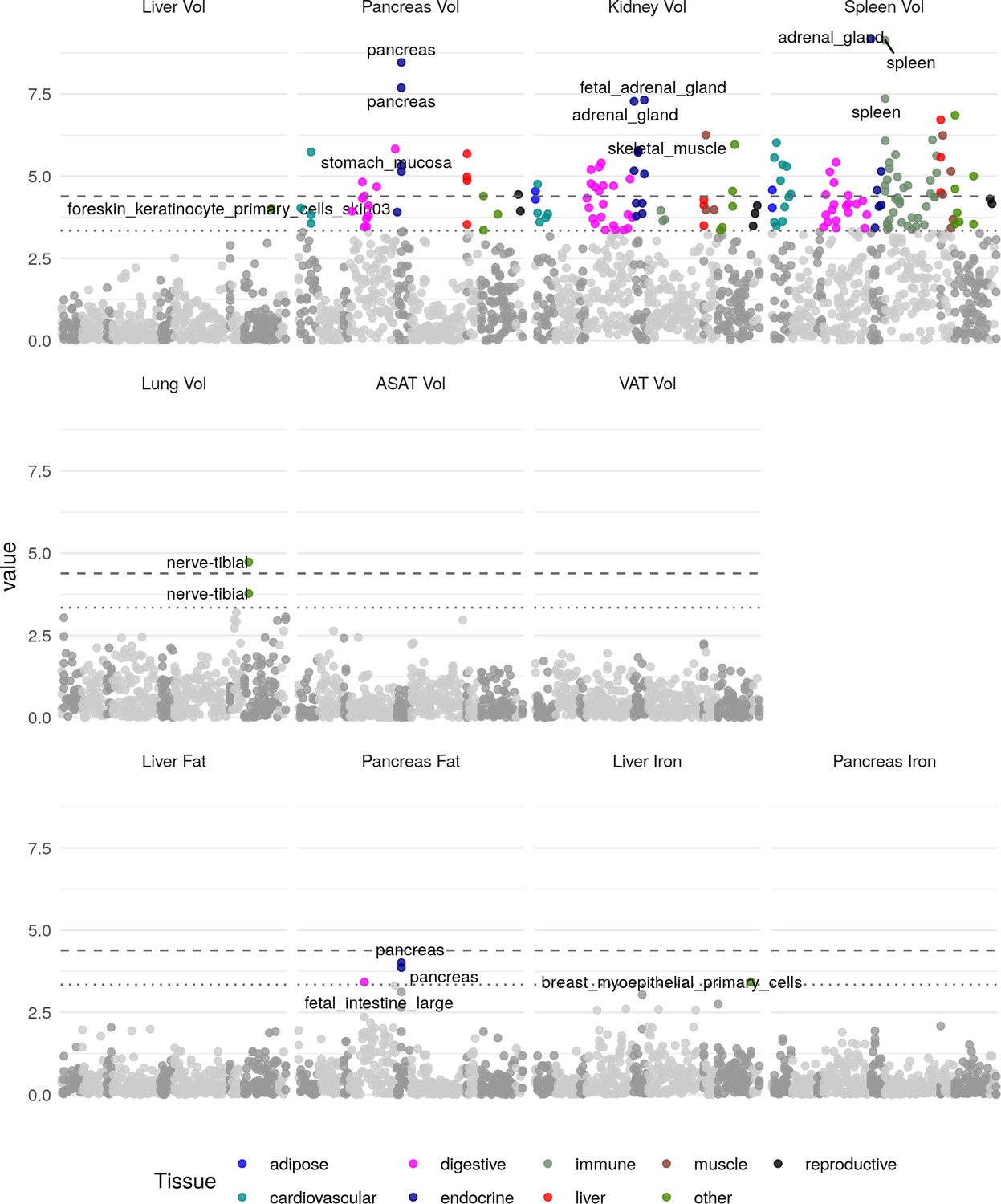
Heritability enrichment in tissues and cell types for annotations based on chromatin accessibility (see Materials and methods).
The top three enrichments for each phenotype passing a trait-wide significance threshold are labelled. Horizontal lines and trait-wide (dotted line) and study-wide (dashed line) significance after Bonferroni correction.
Figure 3—figure supplement 5
Heritability enrichment in tissues and cell types in immune cell types (see Materials and methods).
The top three enrichments for each phenotype passing a trait-wide significance threshold are labelled. Horizontal lines and trait-wide (dotted line) and study-wide (dashed line) significance after Bonferroni correction.
Figure 3—figure supplement 6
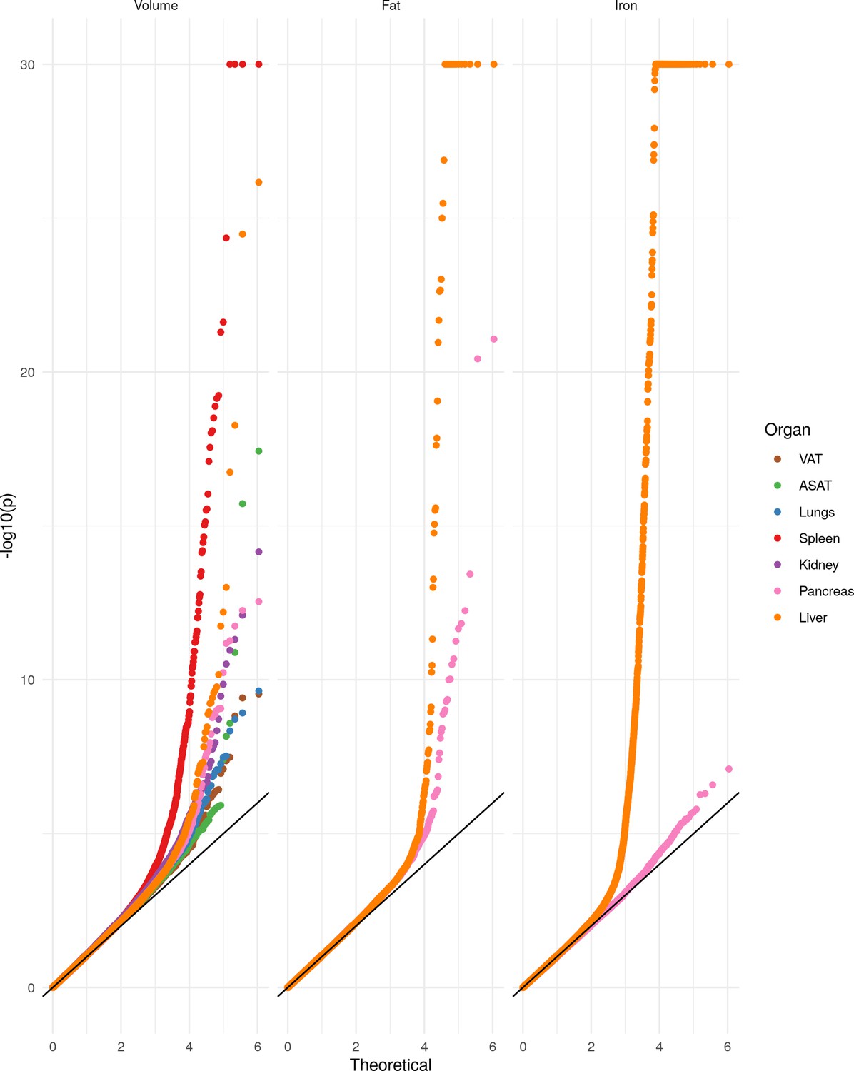
QQ plots calculated based on a set approximately 500,000 LD-pruned, genotyped SNPs per trait.
Tables
Table 1
Study population characteristics.
Age, BMI, and height rows give mean and SD for each population.
| UK biobank cohort (at time of baseline visit) | Imaging cohort (at time of imaging visit) | GWAS cohort (White British Ancestry and passing QC) | ||||
|---|---|---|---|---|---|---|
| Organ volume (DIXON) | Pancreas volume | Pancreas fat and iron | Liver fat and iron | |||
| Number of participants | 502,520 | 38,881* | 32,860 | 31,758 | 25,617 | 32,858 |
| % Female | 54.4 | 51.8 | 51.5 | 51.4 | 51.2 | 51.5 |
| Age | 56.5 (8.1) | 63.7 (7.56) | 63.9 (7.52) | 63.8 (7.52) | 64.2 (7.48) | 63.9 (7.52) |
| BMI (kg/m2) | 27.4 (4.8) | 26.5 (4.39) | 26.5 (4.37) | 26.5 (4.34) | 26.5 (4.31) | 26.5 (4.36) |
| Height (cm) | 168 (9.28) | 169 (9.3) | 169 (9.26) | 169 (9.25) | 169 (9.26) | 169 (9.26) |
| % White British Ancestry | 81.5 | 81.5 | 100 | 100 | 100 | 100 |
-
*Number of imaging participants gives the number with at least one abdominal IDP successfully extracted.
Table 2
Mean and standard deviations for 11 IDPs in our study, and number of independent GWAS associations found at study-wide significance (p<4.54e-9; see Materials and methods).
| Trait | Organ | Combined | Female | Male | # Study-wide significant GWAS hits |
|---|---|---|---|---|---|
| Volume (L) | VAT | 3.92 (2.3) | 2.78 (1.6) | 5.14 (2.3) | 3 |
| ASAT | 8.16 (4.1) | 9.57 (4.3) | 6.64 (3.2) | 1 | |
| Lungs | 2.67 (0.73) | 2.32 (0.53) | 3.03 (0.75) | 5 | |
| Spleen | 0.17 (0.072) | 0.14 (0.054) | 0.2 (0.078) | 29 | |
| Kidney | 0.14 (0.03) | 0.12 (0.023) | 0.16 (0.028) | 9 | |
| Pancreas | 0.06 (0.018) | 0.06 (0.016) | 0.06 (0.019) | 11 | |
| Liver | 1.38 (0.3) | 1.28 (0.25) | 1.49 (0.3) | 11 | |
| Fat (%) | Pancreas | 10.41 (7.9) | 8.34 (6.7) | 12.6 (8.5) | 8 |
| Liver | 5.06 (5) | 4.43 (4.7) | 5.73 (5.2) | 11 | |
| Iron (mg/g) | Pancreas | 0.77 (0.097) | 0.8 (0.1) | 0.75 (0.084) | 0 |
| Liver | 1.22 (0.26) | 1.2 (0.24) | 1.24 (0.28) | 6* |
-
*Due to complex LD structure in this region, we were not able to finemap the HFE locus. We count two signals at this locus (rs1800562 and rs1799945).
Additional files
-
Supplementary file 1
(a) Segmentation performance metrics. (b) Numbers of participants at each stage of the processing pipeline for different scan and data types. (c) Significant PheWAS associations. Only associations which are statistically significant after correction for multiple testing are shown. (d) Significant PHESANT associations. Only associations which are statistically significant after correction for multiple testing are shown. (e) LDSC intercept. (f) Genetic correlations between abdominal IDPs. (g) Genetic correlation between abdominal IDPs and other heritable complex traits. Only associations which are statistically significant after correction for multiple testing are shown. (h) Genome-wide significant lead SNPs. Columns are as follows ● trait: One of: volume, fat or iron ● organ: Organ ● var_index Index variant (in the format chr:pos:ref:alt:build) (All index variants are listed in GRCh37 coordinates) ● rs_id: dbSNP ID ● var_conditional: If a conditional signal, variants conditioned on, in the same format as var_index ● pv P-value ● pp: Probability that the lead SNP is the causal variant ● beta: Effect size (in standard deviations) ● closest_gene: Closest protein-coding gene ● closest_gene_dist: Distance to TSS of closest gene (i) Significant colocalisation with complex trait GWAS signals. (j) Significant colocalisation with gene expression. (k) Genomic control parameter for each trait computed using BOLT-LMM on an LD-pruned set of genotyped SNPs.
- https://cdn.elifesciences.org/articles/65554/elife-65554-supp1-v1.xlsx
-
Transparent reporting form
- https://cdn.elifesciences.org/articles/65554/elife-65554-transrepform-v1.pdf
Download links
A two-part list of links to download the article, or parts of the article, in various formats.
Downloads (link to download the article as PDF)
Open citations (links to open the citations from this article in various online reference manager services)
Cite this article (links to download the citations from this article in formats compatible with various reference manager tools)
Genetic architecture of 11 organ traits derived from abdominal MRI using deep learning
eLife 10:e65554.
https://doi.org/10.7554/eLife.65554


