Inbreeding in a dioecious plant has sex- and population origin-specific effects on its interactions with pollinators
- Kiel University, Institute for Ecosystem Research, Geobotany, Germany
- Bielefeld University, Faculty of Biology, Department of Chemical Ecology, Germany
- German Centre for Integrative Biodiversity Research (iDiv) Halle–Jena–Leipzig, Germany
Figures
Figure 1 with 8 supplements

Graphical sketch of the applied methods.
Each of the eight listed methodologies is illustrated in detail in a figure supplement.
Figure 1—figure supplement 1
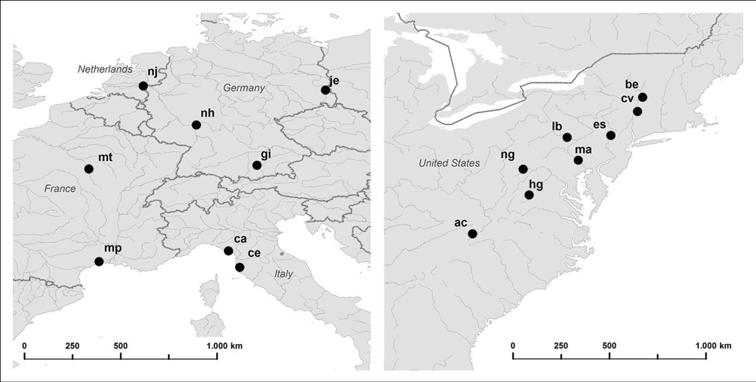
Map of the geographic locations of the sampled European (left) and North American (right) Silene latifolia populations.
Figure 1—figure supplement 2
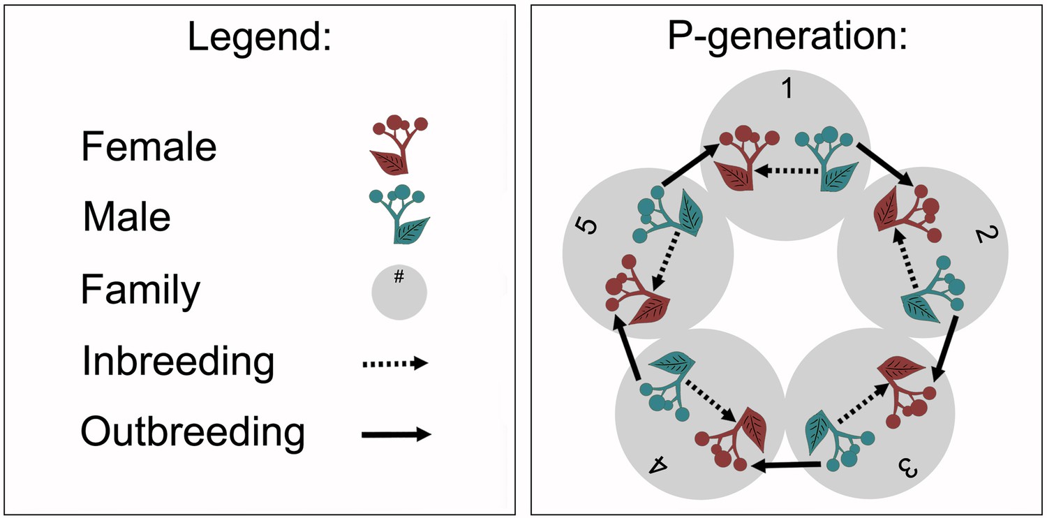
Overview of the experimental crossings within each of the 16 Silene latifolia populations.
The crossings were performed with five families (numbered grey circles). Females (red plants, leaf pointing to left) were fertilised with pollen from males (blue plants, leaf pointing to right) from the same family for inbreeding (dashed arrows), and with pollen from males from a different family for outbreeding (solid arrows). Inbreeding and outbreeding were performed at distinct flowers of the same female individual.
Figure 1—figure supplement 3
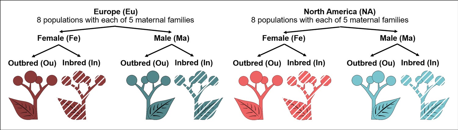
Experimental plants.
Our study involved 320 plant individuals from two origins (Europe, North America) × 8 populations × 5 maternal families × 2 sexes (male, female) × 2 breeding treatments (outbred, inbred).
Figure 1—figure supplement 4
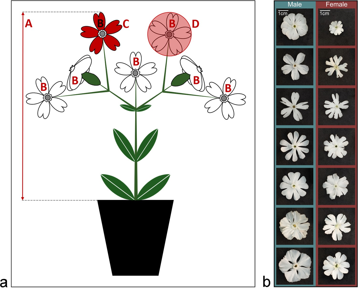
Spatial flower traits.
(a) Spatial flower trait assessment. (A) Maximal synflorescence height above ground, (B) flower number, (C) petal limb area, (D) corolla expansion. (b) Variation in flower shape of Silene latifolia plants in our experiment. Photographs from female (upper row) and male (lower row) flowers with maximal deviation in flower shape were randomly chosen from the entire pool of experimental plants.
Figure 1—figure supplement 5
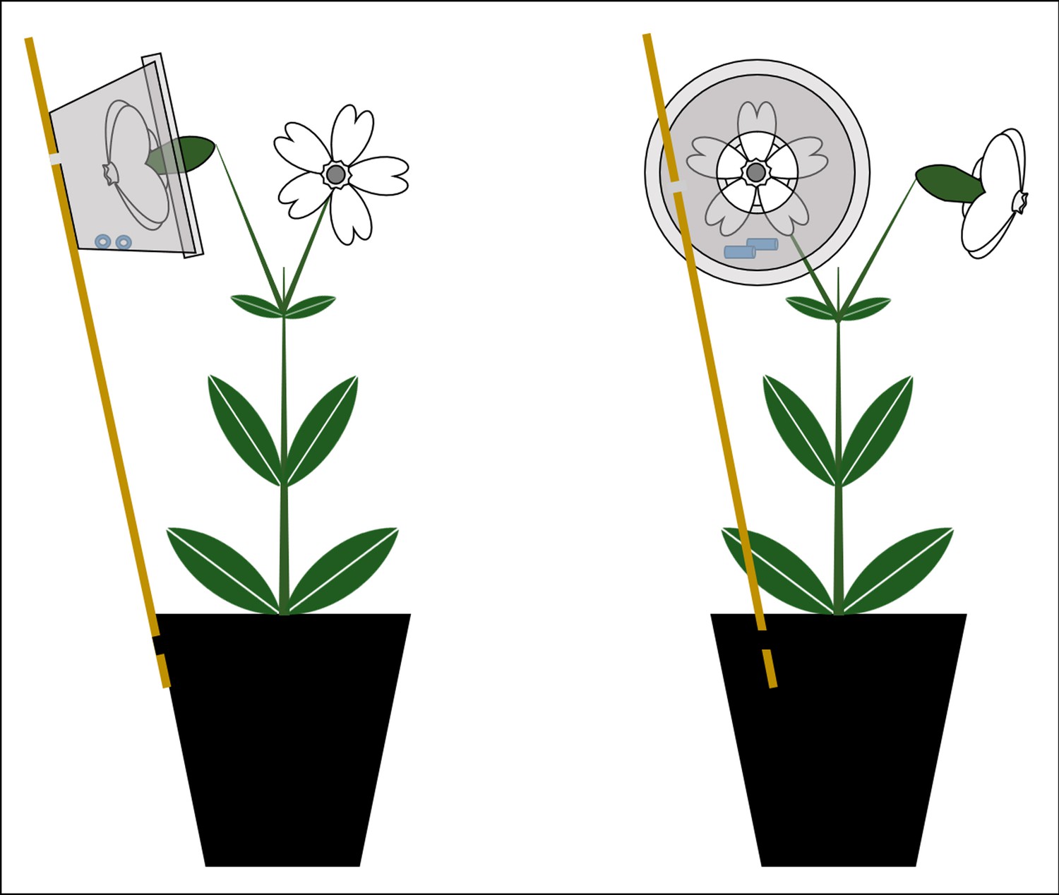
Setup for the collection of headspace volatile organic compounds (VOC) from flowers of Silene latifolia (left: side view, right: front view).
Flowers were inserted into VOC collection units (consisting of 50 mL PE cups with lids, both with 15 mm holes), which were fixed via wooden sticks at the plant pot exterior. Two polydimethylsiloxane (silicone) tubes of standardised size were inserted into the collection units and absorbed VOC for a period of 8 hr.
Figure 1—figure supplement 6
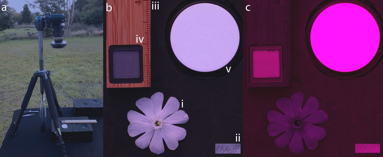
Setup for the acquisition of digital images for flower colour analyses.
The camera was fixed on a tripod positioned on an exact horizontal platform, which was oriented towards the setting sun (a) to take images of flowers in the visible light spectrum (b) and the ultraviolet light spectrum (c). Images included an intact and fully opened flower (i) that was carefully plugged into a black ethylene vinyl acetate sheet equipped with a label (ii), a size standard (iii), a 10% polytetrafluorethylene light standard (iv), and a 99% spectralon light standard (v).
Figure 1—figure supplement 7
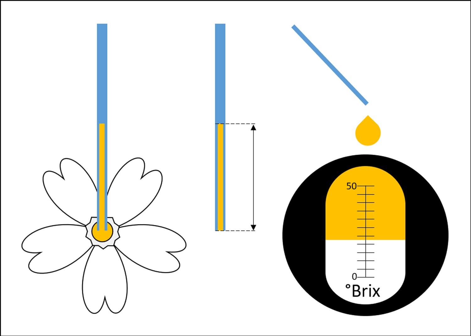
Nectar analyses.
Nectar was extracted into 1 or 2 µL microcapillary tubes. The length of the nectar column was measured with a calliper to determine the exact volume. Nectar sugar content was analysed with a refractometer adjusted for small sample sizes.
Figure 1—figure supplement 8
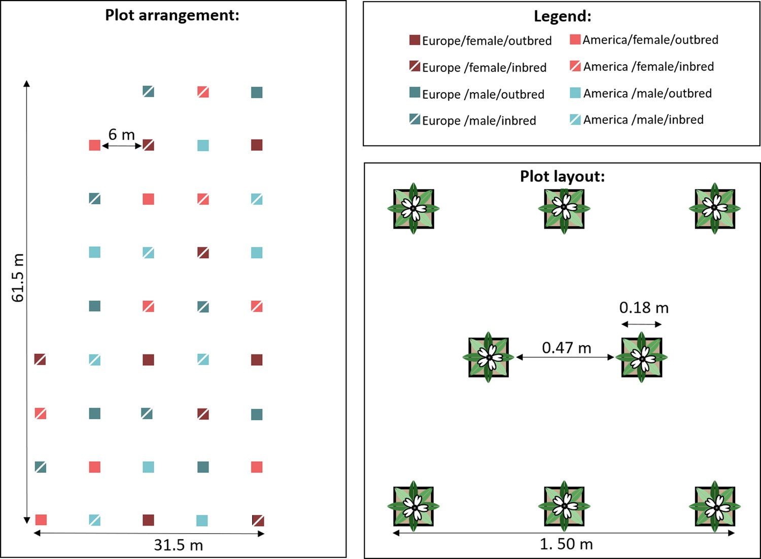
Experimental setup for pollinator observations.
The plots consisted of eight individuals representing all eight populations within one of the eight possible breeding treatment × sex × range combinations. Each of these combinations was replicated five times on the maternal family level, resulting in 40 plots. Plots were spaced at a distance of 6 m to provide pollinators with the choice of visiting plants of specific breeding treatment × sex × range combinations.
Figure 2 with 2 supplements
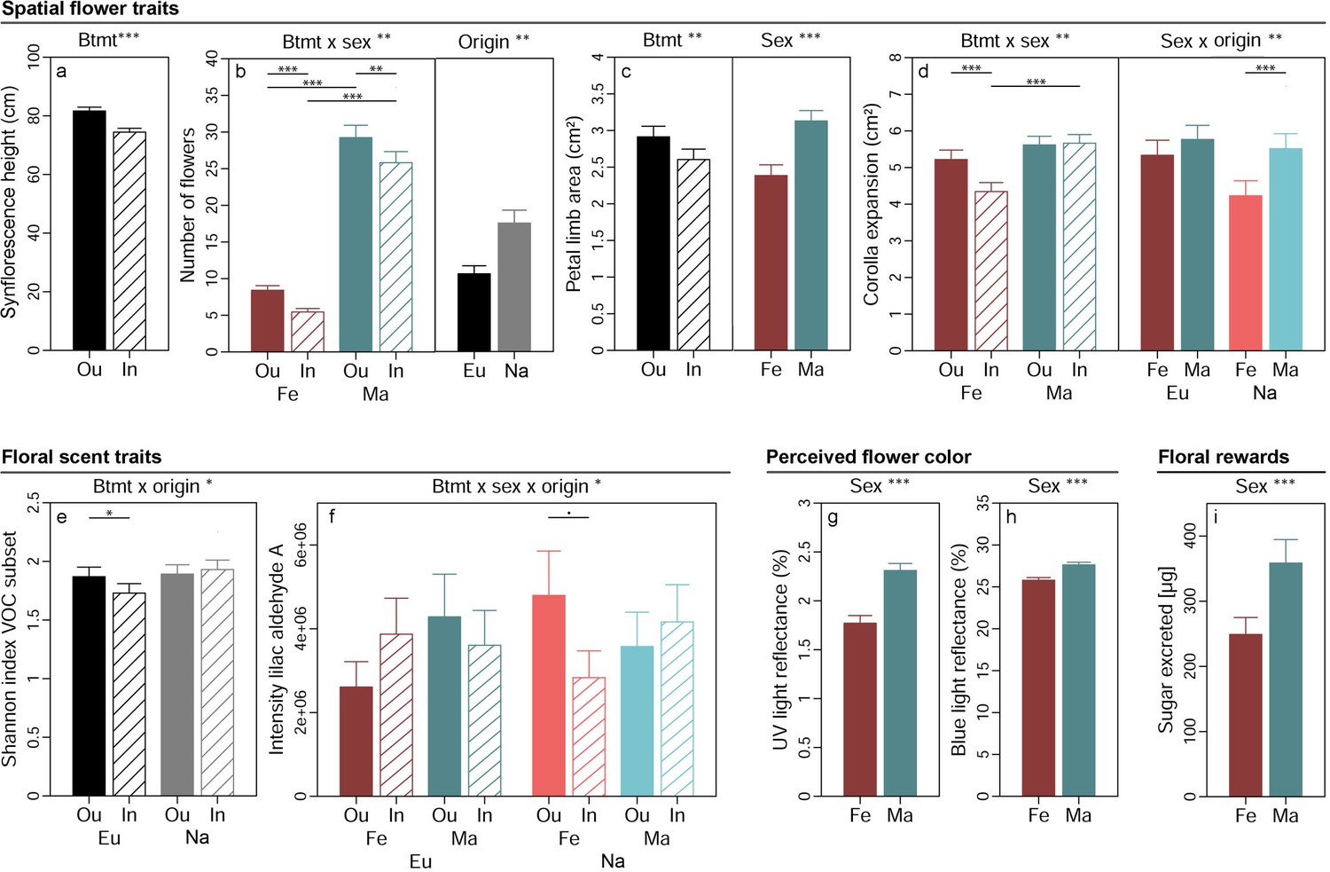
Effects of breeding treatment, sex, and origin on spatial flower traits (a–d), floral scent traits (e–f), flower colour as perceived by crepuscular moths (g–h), and floral rewards in Silene latifolia.
Graphs show estimated marginal means and standard errors for outbred (Ou, filled bars) and inbred (In, open bars), female (Fe, red bars) and male (Ma, blue bars) plants from Europe (Eu, dark coloured bars) and the North America (Na, bright coloured bars). Estimates were extracted from (generalised) linear mixed effects models for significant interaction effects and main effects of factors not involved in an interaction (significance levels based on Wald χ² tests denoted at top of plot). Interaction effect plots additionally indicate significant differences among breeding treatments, sexes, or origins within levels of other factors involved in the respective interaction (estimated based on post hoc comparisons, denoted within plots). Exact sample sizes for all traits are listed in Table 1. Significance levels: ***p<0.001, **p<0.01, *p<0.05, •p<0.06.
Figure 2—figure supplement 1
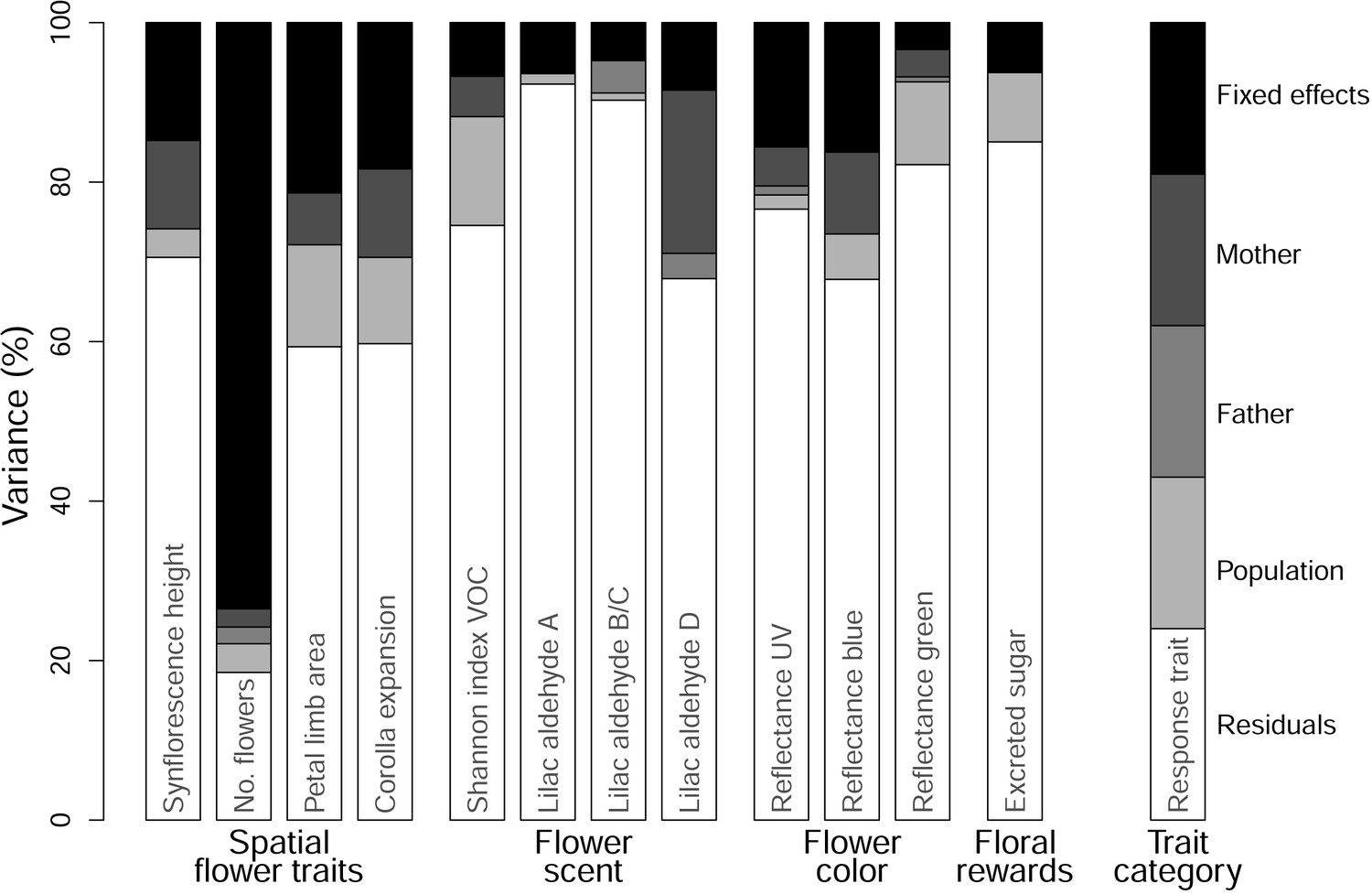
Stacked bar plot illustrating the proportions of variance in floral trait responses explained by fixed effects (black) and the random effects of mother in the P-generation (dark grey), father in the P-generation (medium grey), and population (light grey), as well as the amount of unexplained variance, that is, residuals (white).
Please note that the amount of variation in response variables that is explained by fixed effects exceeds the amount of variance explained by the population random factor in 9 of 12 models.
Figure 2—figure supplement 2
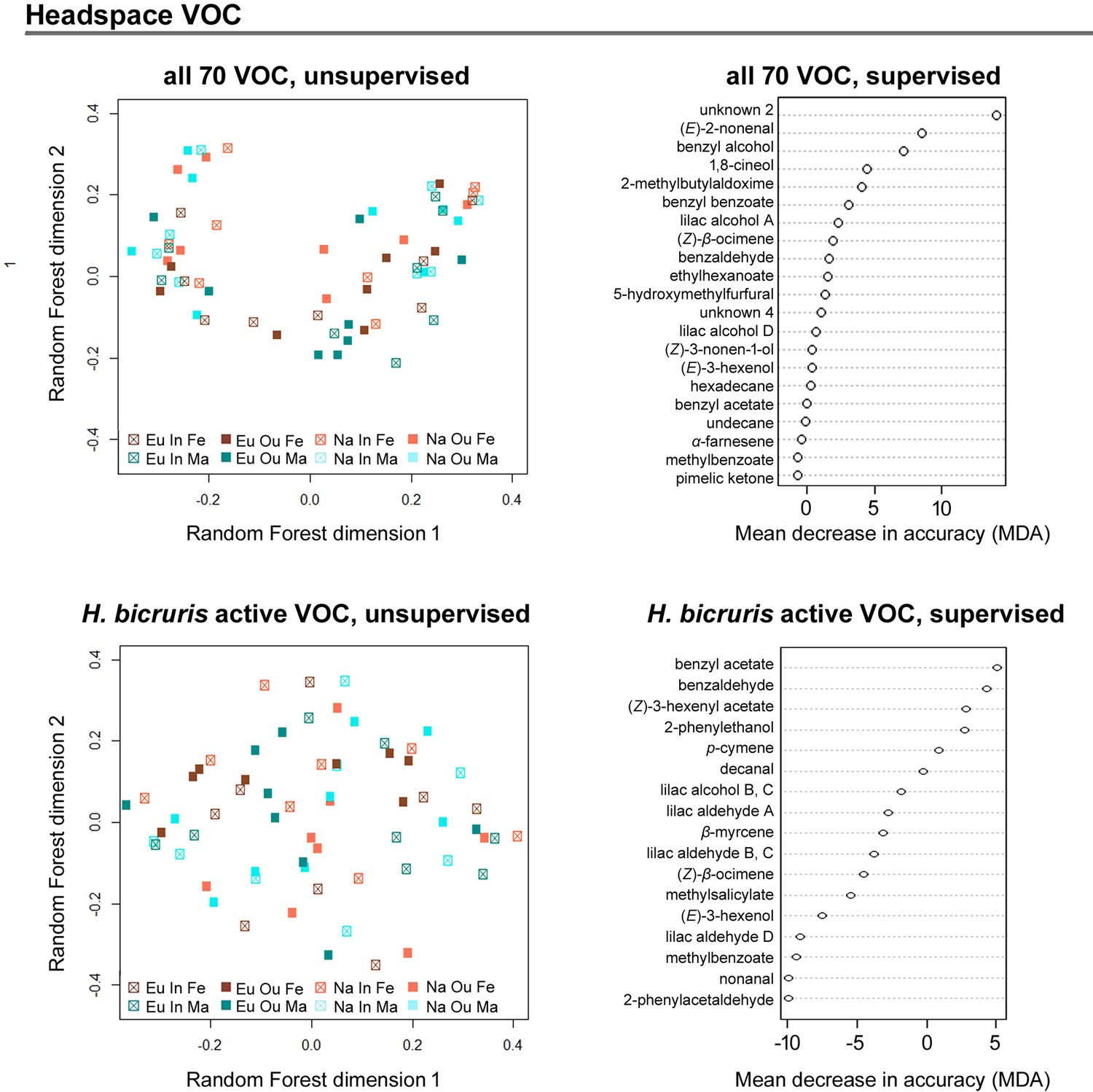
Unsupervised random forest comparison MDS plots for floral headspace volatile organic compounds (VOC, left panel) and supervised random forest importance plots for mean decrease in accuracy (MDA, right panel) for all detected compounds (upper plots) and the subset for compounds that can be detected by Hadena bicruris (lower plots).
Patterns were compared for outbred (Ou, filled squared) and inbred (In, open squares), female (Fe, red) and male (Ma, blue) plants from Europe (Eu, dark coloured) and North America (Na, bright coloured). Each square represents one population, data within populations were averaged to improve clarity.
Figure 3 with 1 supplement

Effects of breeding treatment, sex, and origin on pollinator visitation rates in Silene latifolia.
Graphs show estimated marginal means and standard errors for outbred (Ou, filled bars) and inbred (In, open bars), female (Fe, red bars) and male (Ma, blue bars) plants from Europe (Eu, dark coloured bars) and North America (Us, bright coloured bars). Estimates were extracted for significant interaction effects from the conditional part of generalised linear mixed effects models (significance levels based on Wald χ² -tests denoted at top of plot). Plots additionally indicate significant differences between breeding treatments, sexes, or origins within levels of other factors involved in the respective interaction (estimated based on post -hoc comparisons, denoted within plots). Exact sample sizes for all traits are listed in Table 1. Significance levels: ***p<0.001, **p<0.01, and *p<0.05.
Figure 3—figure supplement 1
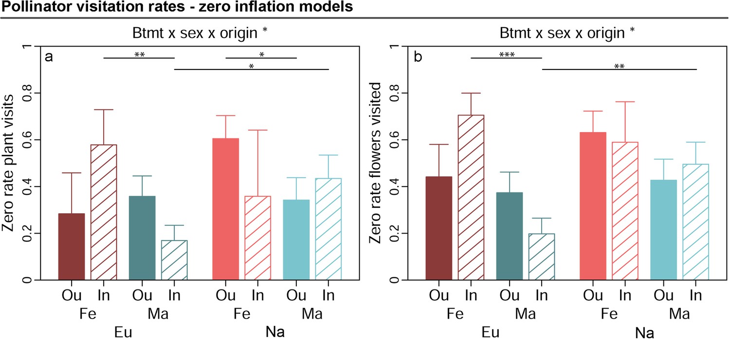
Estimated marginal means for zero scores in pollinator visitation responses (increasing values indicate higher proportion of zeroes in response data) and standard errors for outbred (Ou, filled bars) and inbred (In, open bars), female (Fe, red bars) and male (Ma, blue bars) plants from Europe (Eu, dark coloured bars) and North America (Us, bright coloured bars).
Estimates were extracted for significant interaction effects from the zero inflation part of generalised linear mixed effects models (significance levels based on Wald χ² tests denoted at top of plot). Plots additionally indicate significant differences between breeding treatments, sexes, or origins within levels of other factors involved in the respective interaction (estimated based on post hoc comparisons, denoted within plots). Exact sample sizes for all responses are listed in Table 1. Significance levels: ***p<0.001, **p<0.01, and *p<0.05.
Tables
Table 1
Overview of locations, times, and sample sizes for data acquisition.
| Trait category | Location | Acquisition time (year, month, duration) | Nesting and intended total sample size | Realised total sample size | Replicates per group (breeding treatment × sex × origin combination) | Reason for sample size reduction |
|---|---|---|---|---|---|---|
| Spatial flower traits (synflorescence height, flower number) | Greenhouse and common garden | 2019 Jun., Jul., Aug. 5 days, respectively | Two breeding treatments × 2 sexes × 5 maternal families × 8 populations × 2 origins=320 | 316 | 36–40 | Four individuals died |
| Flower scent | Greenhouse | 2019 Jul. 8 hr | Two breeding treatments × 2 sexes × 3 maternal families × 8 populations × 2 origins=192 | 192 | 23–35 | - |
| Flower colour | Common garden | 2019 Aug. 2 weeks | Two breeding treatments × 2 sexes × 5 maternal families × 8 populations × 2 origins=320 | 286 | 23–25 | Four individuals died, no flowers available for remaining plants |
| Spatial flower traits (petal limb area and expansion) | Common garden | 2019 Aug. 2 weeks | Two breeding treatments × 2 sexes × 5 maternal families × 8 populations × 2 origins=320 | 286 | 23–35 | Four individuals died, no flowers available for remaining plants |
| Pollinator visitation rates | Field site | 2020 May–Jul. 8 weeks | Two breeding treatments × 2 sexes × 5 maternal families × 8 populations × 2 origins=320 | 316 | 36–40 | Four individuals died |
| Floral rewards | Common garden | 2020 Aug. 4 weeks | Two breeding treatments × 2 sexes × 5 maternal families × 8 populations × 2 origins=320 | 280 | 30–40 | Four individuals died, no flowers available for remaining plants |
Table 2
Overview and results of statistical analyses with (generalised) linear mixed effects models.
The table summarises the model types and error distributions used for each of the responses (printed in subscript), the parameter estimates on the link function scale with significance levels assessed based on Wald χ² tests for all fixed effects (***p<0.001, **p<0.01, and *p<0.05 printed in bold), and random effect variances (printed in italic). For zero inflated responses, estimates from the conditional model parts appear in the first line and estimates from zero inflation model parts in the second line. All listed fixed effects consume 1 degree of freedom.
| Intercept | Btmt [outbred –inbred] | Sex [female –male] | Origin [Europe –US] | Btmt × sex | Btmt × origin | Sex × origin | Btmt × sex × origin | Latitude | Plant age | Obs. time | Pop | Pop: mother | Pop : father | Plot | Obs. trial | |
|---|---|---|---|---|---|---|---|---|---|---|---|---|---|---|---|---|
| Spatial flower traits | ||||||||||||||||
| Synflorescence heightLMM(G) | 81.03 | 3.56*** | −0.40NS | 1.84 | 0.67 | 0.11 | 1.07Ns | −0.15 | 1.00 | Nt. | Nt. | 5.42 | 16.76 | 0.00 | Nt. | Nt. |
| No. flowersGLMM(NBQ) | 2.61 | 0.14*** | −0.70*** | −0.25** | 0.08** | −0.04 | 0.01 | 0.01 | 0.12 | Nt. | Nt. | 0.03 | 0.02 | 0.02 | Nt. | Nt. |
| Petal limb areaLMM(G) | 2.76 | 0.16** | −0.38*** | 0.07 | 0.06 | 0.04 | 0.10 | 0.03 | 0.19 | Nt. | Nt. | 0.15 | 0.08 | 0.00 | Nt. | Nt. |
| Corolla expansionLMM(G) | 5.21 | 0.21** | −0.44*** | 0.33 | 0.23** | 0.02 | 0.21** | 0.11 | 0.06 | Nt. | Nt. | 0.29 | 0.30 | 0.00 | Nt. | Nt. |
| Flower scent traits | ||||||||||||||||
| Shannon index VOCLMM(G) | 1.86 | 0.03 | −0.13* | −0.06 | 0.01 | 0.04 | 0.02 | 0.01 | 0.03 | −0.02* | Nt. | 0.01 | 0.00 | 0.00 | Nt. | Nt. |
| Lilac aldehyde AZI-GLMM(NBQ) | 15.11 | 0.02 | −0.06 | 0.02 | 0.01 | −0.08 | −0.04 | −0.16* | 0.01 | −0.08 | Nt. | 0.01 | 0.00 | 0.00 | Nt. | Nt. |
| −1.93*** | Nt. | Nt. | Nt. | Nt. | Nt. | Nt. | Nt. | Nt. | Nt. | Nt. | Nt. | Nt. | Nt. | Nt. | Nt. | |
| Lilac aldehyde B/CZI-GLMM(NBL) | 15.78 | −0.08 | −0.09 | 0.12 | 0.06 | −0.10 | −0.01 | −0.03 | −0.09 | −0.03 | Nt. | 0.01 | 0.00 | 0.03 | Nt. | Nt. |
| −1.93*** | Nt. | Nt. | Nt. | Nt. | Nt. | Nt. | Nt. | Nt. | Nt. | Nt. | Nt. | Nt. | Nt. | Nt. | Nt. | |
| Lilac aldehyde DZI-GLMM(NBQ) | 13.70 | −0.05 | 0.14 | −0.07 | −0.09 | −0.16 | −0.06 | −0.08 | 0.08 | −0.17 | Nt. | 0.00 | 2.75 | 0.47 | Nt. | Nt. |
| 0.02Ns | Nt. | Nt. | Nt. | Nt. | Nt. | Nt. | Nt. | Nt. | Nt. | Nt. | Nt. | Nt. | Nt. | Nt. | Nt. | |
| Flower colour | ||||||||||||||||
| Reflectance UVLMM(G) | 2.04 | −0.05 | −0.27*** | 0.05 | 0.04 | 0.08Ns | −0.04 | 0.02 | 0.01 | Nt. | Nt. | 0.01 | 0.03 | 0.01 | Nt. | Nt. |
| Reflectance blueLMM(G) | 26.72 | −0.02 | −0.95*** | 0.10 | 0.24 | 0.05 | 0.21 | 0.14Ns | 0.47 | Nt. | Nt. | 0.47 | 0.85 | 0.00 | Nt. | Nt. |
| Reflectance greenLMM(G) | 39.87 | −0.10 | −0.19 | 0.40 | 0.26 | 0.17 | 0.12 | 0.31Ns | 0.05 | Nt. | Nt. | 1.12 | 0.37 | 0.07 | Nt. | Nt. |
| Floral rewards | ||||||||||||||||
| Excreted sugarLMM(G) | 5.70 | 0.03 | −0.18*** | −0.08 | 0.04 | −0.02 | −0.02 | 0.04 | 0.04 | Nt. | Nt. | 0.07 | 0.00 | 0.00 | Nt. | Nt. |
| Pollinator visitation | ||||||||||||||||
| No. plant visitsZI-GLMM(P) | 0.28 | 0.09 | −0.67*** | 0.09 | 0.22 | −0.20 | −0.16 | −0.29* | Nt. | Nt. | −0.11* | Nt. | Nt. | Nt. | 0.27 | 0.15 |
| −0.48Ns | 0.05 | 0.29 | −0.21 | −0.11 | −0.11 | 0.10 | −0.46* | Nt. | Nt. | 0.10 | Nt. | Nt. | Nt. | 0.14 | 0.44 | |
| No. flowers visitedZI-GLMM(P) | 0.79 | 0.04 | −0.56*** | −0.03 | 0.34* | −0.23 | −0.22 | −0.46** | Nt. | Nt. | 0.19*** | Nt. | Nt. | Nt. | 0.68 | 0.23 |
| −0.09Ns | −0.04 | 0.47** | −0.23 | −0.19 | −0.02 | 0.17 | −0.31* | Nt. | Nt. | 0.47** | Nt. | Nt. | Nt. | 0.16 | 0.47 |
-
Abbreviations. Btmt: breeding treatment, LMM: linear mixed effects model, (NBQ): negative binomial distribution with quadratic parametrisation and log-link, (NBL): negative binomial distribution with linear parametrisation and log-link, No.: number, Nt.: not tested, GLMM: generalised linear mixed effects model, Obs: observation, (P): Poisson distribution with log-link, Pop: population, ZI-GLMM: zero inflation generalised mixed effects model, (G): Gaussian distribution with identity link.
Additional files
-
Supplementary file 1
Mean ± SE abundance (e-06) of 70 volatile organic compounds (VOC) emitted by Silene latifolia plants in all breeding treatment × sex × origin combinations, as determined by silicone tubing headspace collection combined with thermal desorption–gas chromatography–mass spectrometry.
The 20 VOC, which evidently trigger antennal responses in Hadena bicruris (Dötterl et al., 2006) and were thus analysed as a sub-dataset, are highlighted in bold.
- https://cdn.elifesciences.org/articles/65610/elife-65610-supp1-v2.docx
-
Transparent reporting form
- https://cdn.elifesciences.org/articles/65610/elife-65610-transrepform-v2.pdf
Download links
A two-part list of links to download the article, or parts of the article, in various formats.
Downloads (link to download the article as PDF)
Open citations (links to open the citations from this article in various online reference manager services)
Cite this article (links to download the citations from this article in formats compatible with various reference manager tools)
Inbreeding in a dioecious plant has sex- and population origin-specific effects on its interactions with pollinators
eLife 10:e65610.
https://doi.org/10.7554/eLife.65610


