Visualizing anatomically registered data with brainrender
- UCL Sainsbury Wellcome Centre, United Kingdom
- Institute of Neuroscience, Technical University of Munich, Germany
- Max Planck Institute of Neurobiology, Research Group of Sensorimotor Control, Germany
- Munich Cluster for Systems Neurology (SyNergy), Germany
Figures
Figure 1

Design principles.
(A) Schematic illustration of how different types of data can be loaded into brainrender using either brainrender’s own functions, software packages from the BrainGlobe suite, or custom Python scripts. All data loaded into brainrender is converted to a unified format, which simplifies the process of visualizing data from different sources. (B) Using brainrender with different atlases. Visualization of brain atlas data from three different atlases using brainrender. Left, Allen atlas of the mouse brain showing the superficial (SCs) and motor (SCm) subdivisions of the superior colliculus and the Zona Incerta (data from Wang et al., 2020). Middle, visualization of the cerebellum and tectum in the larval zebrafish brain (data from Kunst et al., 2019). Right, visualization of the precentral gyrus, postcentral gyrus, and temporal lobe of the human brain (data from Ding et al., 2016). (C) The brainrender GUI. Mouse, human, and zebrafish larvae drawings from scidraw.io (doi.org/10.5281/zenodo.3925991, doi.org/10.5281/zenodo.3926189, doi.org/10.5281/zenodo.3926123).
Figure 2
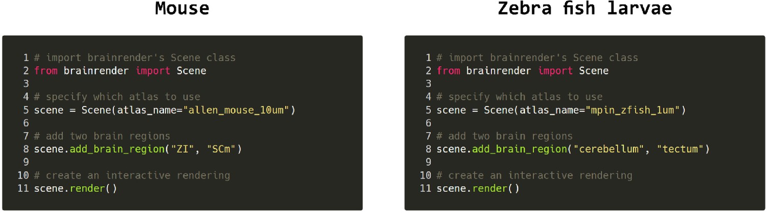
Code examples.
Example python code for visualizing brain regions in the mouse and larval zebrafish brains. The same commands can be used for both atlases and switching between atlases can be done by simply specifying which atlas to use when creating the visualization. Further examples can be found in brainrender’s GitHub repository.
Figure 3
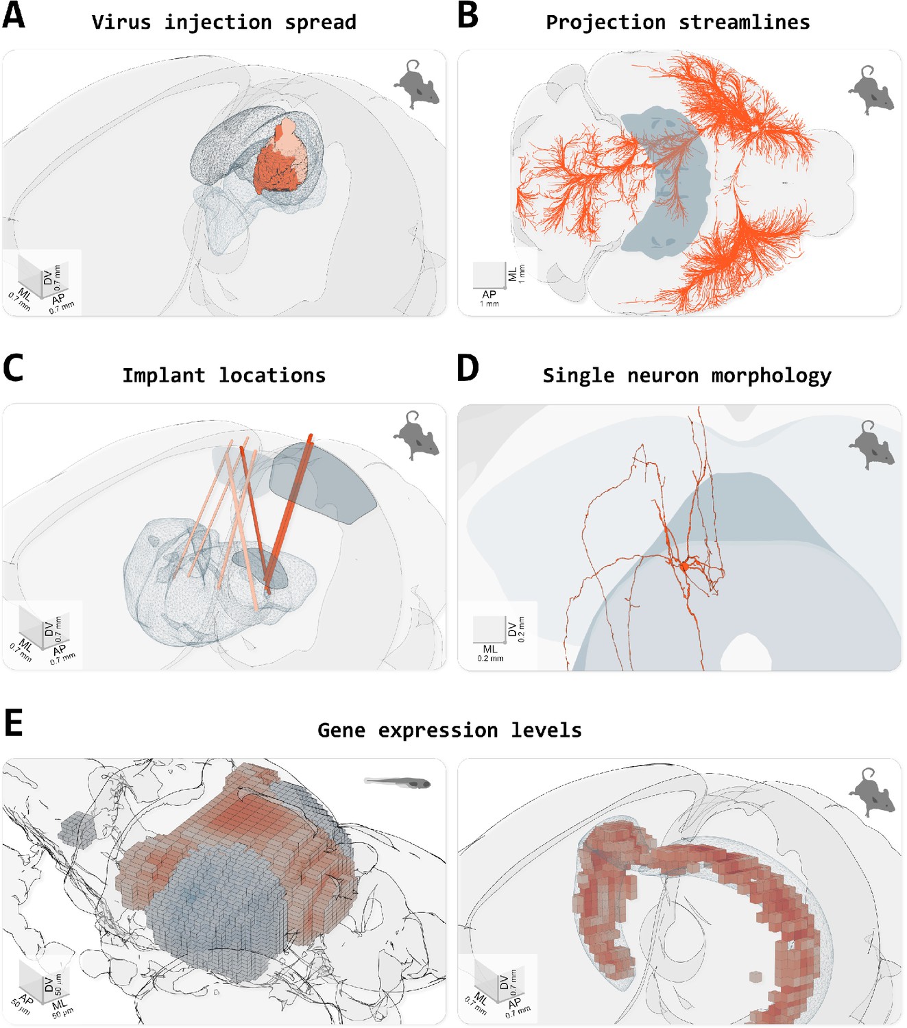
Visualizing different types of data in brainrender.
(A) Spread of fluorescence labeling following viral injection of AAV2-CRE-eGPF in the superior colliculus of two FLEX-TdTomato mice. 3D objects showing the injection sites were created using custom python scripts following acquisition of a 3D image of the entire brain with serial two-photon tomography and registration of the image data to the atlas’ template (with brainreg, Tyson et al., 2020a). (B) Streamlines visualization of efferent projections from the mouse primary motor cortex following injection of an anterogradely transported virus expressing fluorescent proteins (original data from Oh et al., 2014), downloaded from (Neuroinformatics NL with brainrender). (C) Visualization of the location of several implanted neuropixel probes from multiple mice (data from Steinmetz et al., 2019). Dark salmon colored tracks show probes going through both primary/anterior visual cortex (VISp/VISa) and the dorsal lateral geniculate nucleus of the thalamus. (D) Single periaqueductal gray (PAG) neuron. The PAG and superior colliculus are also shown. The neuron’s morphology was reconstructed by targeting the expression of fluorescent proteins in excitatory neurons in the PAG via an intersectional viral strategy, followed by imaging of cleared tissue and manual reconstruction of the neuron’s morphology with Vaa3D software. Data were registered to the Allen atlas with SHARPTRACK (Shamash et al., 2018). The 3D data was saved as a .stl file and loaded directly into brainrender. (E) Gene expression data. Left, expression of genes ‘brn3c’ and ‘nk1688CGt’ in the tectum of the larval zebrafish brain (gene expression data from fishatlas.neuro.mpg.de, 3D objects created with custom python scripts). Right, expression of gene ‘Gpr161’ in the mouse hippocampus (gene expression data from Wang et al., 2020), downloaded with brainrender (3D objects created with brainrender). Colored voxels show voxels with high gene expressions. The CA1 field of the hippocampus is also shown.
Figure 4
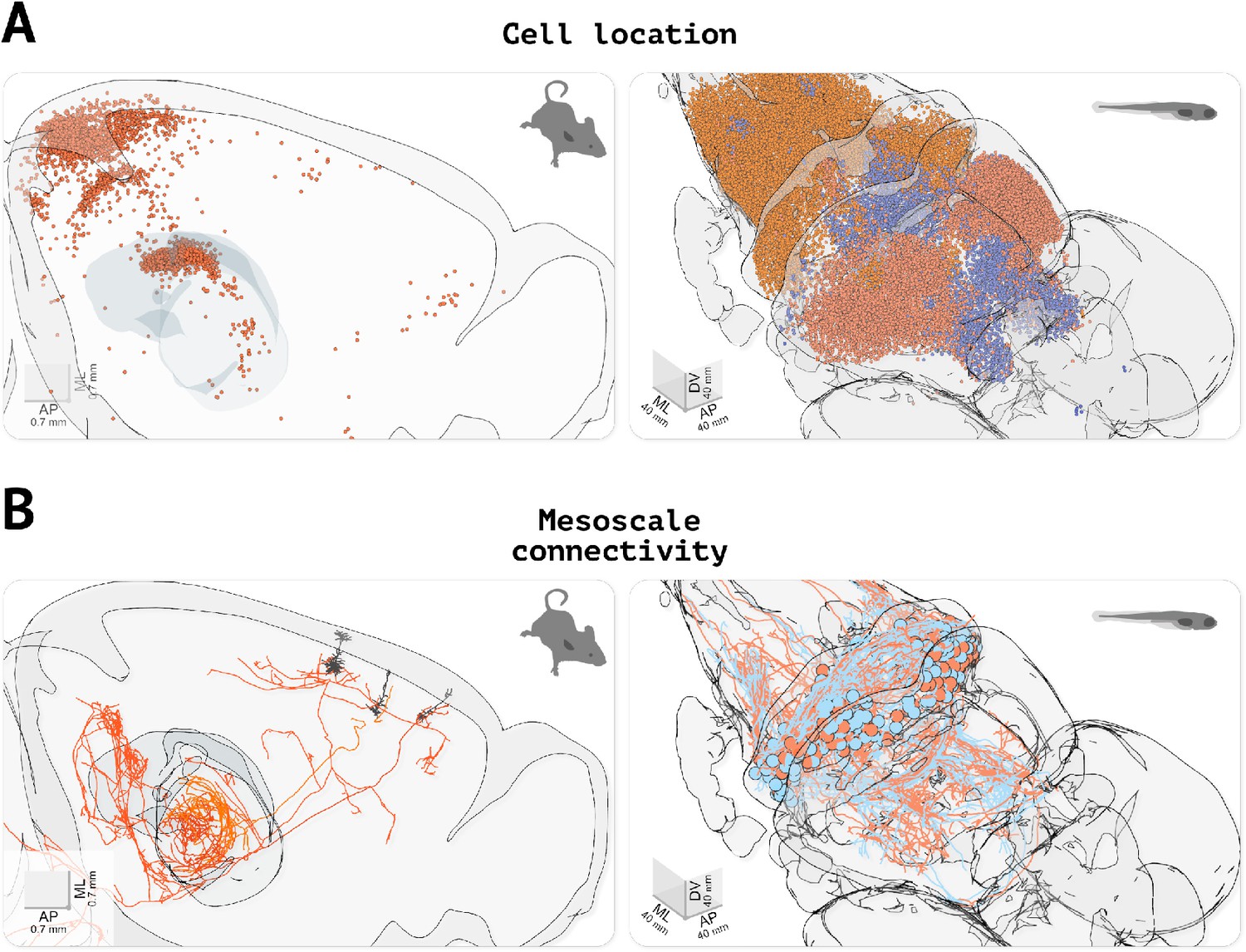
Visualizing cell location and morphological data.
(A) Visualizing the location of labeled cells. Left, visualization of fluorescently labeled cells identified using cellfinder (data from Tyson and Rousseau, 2020b). Right, visualization of functionally defined clusters of regions of interest in the brain of a zebrafish larvae during a visuomotor task (data from Markov et al., 2020). (B) Visualizing neuronal morphology data. Left, three secondary motor cortex neurons projecting to the thalamus (data from Winnubst et al., 2019, downloaded with morphapi from neuromorpho.org, Ascoli et al., 2007). Right, morphology of cerebellar neurons in larval zebrafish (data from Kunst et al., 2019), (downloaded with morphapi). In the left panel of (A and B), the brain outline was sliced along the midline to expose the data.
Figure 5

Code examples.
(A) Example code to visualize a set of labeled cells coordinates using the Points actor class. (B) Code example illustrating how to override brainrender’s default settings and how to use custom camera settings. (C) Code example showing how custom mesh objects saved as .obj and .stl files can be visualized in brainrender. (D) Example usage of brainrender’s Animation class to create custom animations. Further examples can be found in brainrender’s GitHub repository.
Figure 6
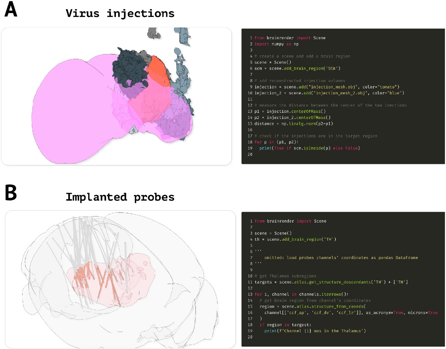
Advanced code examples.
(A) Example code to measure the distance between actors and if a given actor is contained in a target brain region. Left: virus injection volumes (red and gray) reconstructed from virus injections targeted at the superior colliculus (magenta). Gray colored injection volumes show data from the Allen Mouse Connectome Oh et al., 2014. Right: example code to measure the distance between the center of two brainrender actors and to check if an actor’s center is contained in a brain region of interest. (B) Code example illustrating how check if a point (e.g., representing a labeled cell) is in a brain region of interest. Left: visualization of reconstructed probe positions from several individual animals, data from Steinmetz et al., 2019. Probe channels located in the thalamus (red) are highlighted. Right: example code showing how to use BrainGlobe’s AtlasAPI to verify whether a point (here representing a probe channel) is contained in a brain region of interest or any of its substructures. Further examples can be found in brainrender’s GitHub repository.
Videos
Video 1
Example brainrender GUI usage.
Short demonstration of how brainrender's GUI can be used to interactively visualize brain regions, labeled cells, and custom meshes.
Video 2
Animated video created with brainrender.
Visualization of neuronal morphologies for two layer 5b pyramidal neurons in the secondary motor area of the mouse brain. Winnubst et al., 2019, downloaded with morphapi from neuromorpho.org. The secondary motor area and thalamus are also shown.
Video 3
Animated video created with brainrender.
Frontal view of all brain regions in the Allen Mouse Brain atlas as the brain is progressively 'sliced' in the rostro-caudal direction.
Video 4
Animated video created with brainrender.
Visualization of the location of three implanted neuropixel probes from multiple mice (data from Steinmetz et al., 2019). Every 0.5 s, a subset of the probes’ electrodes that detected a neuron's action potential are shown in salmon to visualize neuronal activity.
Video 5
Animated video created with brainrender showing the location of cells labeled by targeted expression of a fluorescent protein identified with cellfinder (data from Tyson et al., 2020a).
In dark blue: streamline visualization of efferent projections from the retrosplenial cortex following injection of an anterogradely transported virus expressing fluorescent proteins (data from Oh et al., 2014).
Tables
Table 1
Machine configurations used for benchmark tests.
| N | OS | CPU | GPU |
|---|---|---|---|
| 1 | Macos Mojave 10.14.6 | 2.3 ghz Intel Core i9 | Radeon Pro 560 × 4 GB GPU |
| 2 | Ubuntu 18.04.2 LTS x86 64 | Intel i7-8565U (x) @ 4.5 ghz | NO GPU |
| 3 | Windows 10 | Intel(R) Core i7-7700HQ 2.8 ghz | NO GPU |
| 4 | Windows 10 | Intel(R) Xeon(R) CPU E5-2643 v3 3.4 ghz | NVIDIA geforce GTX 1080 Ti |
Table 2
Benchmark tests results.
The number of actors refers to the total number of elements rendered, and the number of vertices refers to the total number of mesh vertices in the rendering.
| Test | Machine | GPU | # actors | # vertices | FPS | Run duration |
|---|---|---|---|---|---|---|
| 10 k cells | 1 | Yes | 3 | 1,029,324 | 24.76 | 0.81 |
| 2 | No | 3 | 1,029,324 | 22.46 | 1.16 | |
| 3 | No | 3 | 1,029,324 | 20.00 | 1.41 | |
| 4 | Yes | 3 | 1,029,324 | 100.00 | 1.34 | |
| 100 k cells | 1 | Yes | 3 | 9,849,324 | 18.87 | 3.23 |
| 2 | No | 3 | 9,849,324 | 14.91 | 4.34 | |
| 3 | No | 3 | 9,849,324 | 0.43 | 7.94 | |
| 4 | Yes | 3 | 9,849,324 | 1.20 | 1.13 | |
| 1 M cells | 1 | Yes | 3 | 98,049,324 | 2.65 | 31.01 |
| 2 | No | 3 | 98,049,324 | 2.55 | 96.49 | |
| 3 | No | 3 | 98,049,324 | 0.03 | 86.75 | |
| 4 | Yes | 3 | 9,8049,324 | 0.13 | 36.57 | |
| Slicing 10 k cells | 1 | Yes | 3 | 237,751 | 37.64 | 0.96 |
| 2 | No | 3 | 237,751 | 39.10 | 1.25 | |
| 3 | No | 3 | 237,751 | 26.32 | 1.88 | |
| 4 | Yes | 3 | 237,751 | 200.00 | 1.34 | |
| Slicing 100 k cells | 1 | Yes | 3 | 276,092 | 31.79 | 7.77 |
| 2 | No | 3 | 276,092 | 25.98 | 9.09 | |
| 3 | No | 3 | 276,092 | 21.28 | 16.88 | |
| 4 | Yes | 3 | 276,092 | 111.11 | 9.65 | |
| Slicing 1 M cells | 1 | Yes | 3 | 275,069 | 11.23 | 91.31 |
| 2 | No | 3 | 275,069 | 5.39 | 104.79 | |
| 3 | No | 3 | 275,069 | 5.03 | 158.99 | |
| 4 | Yes | 3 | 275,069 | 37.04 | 97.43 | |
| Brain regions | 1 | Yes | 1678 | 1,864,388 | 9.38 | 11.78 |
| 2 | No | 1678 | 1,864,388 | 7.61 | 27.40 | |
| 3 | No | 1678 | 1,864,388 | 6.49 | 46.79 | |
| 4 | Yes | 1678 | 1,864,388 | 11.90 | 35.83 | |
| Animation | 1 | Yes | 8 | 96,615 | 9.91 | 18.98 |
| 2 | No | 8 | 96,615 | 22.12 | 12.63 | |
| 3 | No | 8 | 96,615 | 15.15 | 11.92 | |
| 4 | Yes | 8 | 96,615 | 47.62 | 12.29 | |
| Volume | 1 | Yes | 12 | 49,324 | 1.79 | 2.31 |
| 2 | No | 12 | 49,324 | 1.66 | 1.95 | |
| 3 | No | 12 | 49,324 | 3.55 | 2.15 | |
| 4 | Yes | 12 | 49,324 | 23.26 | 1.21 |
Key resources table
| Reagent type (species) or resource | Designation | Source or reference | Identifiers | Additional information |
|---|---|---|---|---|
| Software, algorithm | Numpy | https://doi.org/10.1038/s41586-020-2649-2 | RRID:SCR_008633 | |
| Software, algorithm | Vtk | https://doi.org/10.1016/j.softx.2015.04.001 | RRID:SCR_015013 | |
| Software, algorithm | Vedo | https://zenodo.org/record/4287635 | ||
| Software, algorithm | BrainGlobe Atlas API | https://doi.org/10.21105/joss.02668 | ||
| Software, algorithm | Pandas | https://doi.org/10.5281/zenodo.3509134 | ||
| Software, algorithm | Matplotlib | doi: 10.1109/MCSE.2007.55 | RRID:SCR_008624 | |
| Software, algorithm | Jupyter | doi:10.3233/978-1-61499-649-1-87 | RRID:SCR_018416 |
Additional files
Download links
A two-part list of links to download the article, or parts of the article, in various formats.
Downloads (link to download the article as PDF)
Open citations (links to open the citations from this article in various online reference manager services)
Cite this article (links to download the citations from this article in formats compatible with various reference manager tools)
Visualizing anatomically registered data with brainrender
eLife 10:e65751.
https://doi.org/10.7554/eLife.65751


