Cortico-autonomic local arousals and heightened somatosensory arousability during NREMS of mice in neuropathic pain
- Department of Fundamental Neurosciences, Faculty of Biology and Medicine, University of Lausanne, Switzerland
- Pain Center, Department of Anesthesiology, Lausanne University Hospital (CHUV), Switzerland
- Sleep Medicine Unit, Neurocenter of Southern Switzerland, Civic Hospital (EOC) of Lugano, Switzerland
Figures
Figure 1 with 1 supplement
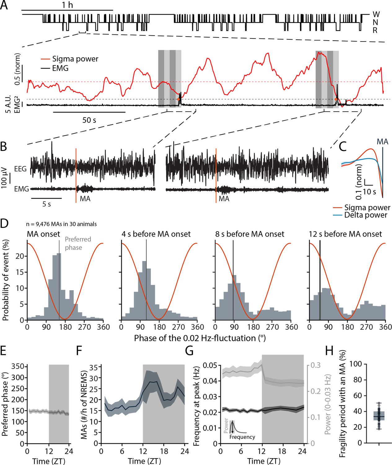
Microarousals (MAs) are time-locked to the trough of the 0.02 Hz-fluctuation corresponding to the non-rapid eye movement sleep (NREMS) fragility period.
(A) Representative mouse hypnogram, W: wakefulness; N: NREMS; R: rapid eye movement sleep (REMS); with an NREMS bout expanded below to indicate the 0.02 Hz-fluctuation in sigma power (red) and the timing of two MAs in the EMG (black). Vertical bars show 4 × 4-s time windows at, and prior to the onset of, the MAs that were used for phase analysis. (B) Two examples of an MA. The MA onset was set at the beginning of phasic EMG activity (orange vertical line). (C) Mean sigma (10–15 Hz) and delta (1–4 Hz) power dynamics preceding the onset of an MA. (D) Histograms of the phase angle values of the 0.02 Hz-fluctuation at specific time points relative to the onset of an MA. The red line represents the corresponding phase of the fluctuation at each bin. (E) Preferred phase of the 0.02 Hz-fluctuation at MA onset across time of day in hourly bins (dark phase, shaded, ZT, Zeitgeber time). (F) Density of MAs (per hour of NREMS) across the light-dark cycle. (G) Parameters of the 0.02 Hz-fluctuation (frequency at peak and power, see inset for illustration) across the light-dark cycle. (H) Proportion of fragility periods (corresponding to phase values from 90 to 270°, see panel D) containing an MA. For statistical analysis for this and all subsequent figures, please consult the Supplementary file 1.
-
Figure 1—source data 1
Source data for Figure 1C–H.
There is one .csv file for each panel except (G). In case of the two datasets used in panel (G), one .csv file for each dataset is generated and appropriately labeled. Additionally, a commented .pdf file with test statistics and p values is provided.
- https://cdn.elifesciences.org/articles/65835/elife-65835-fig1-data1-v3.zip
Figure 1—figure supplement 1
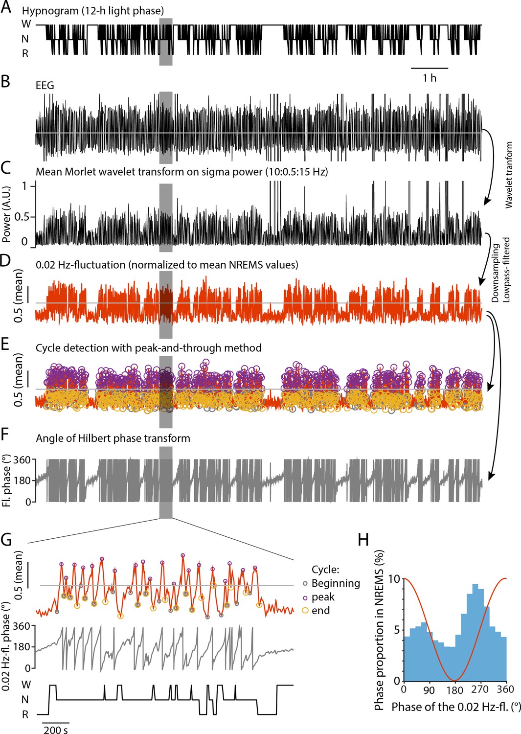
Methodological illustrations regarding analysis of the infraslow 0.02 Hz-fluctuation.
(A) 12 hr hypnogram obtained from visual scoring of EEG/EMG recordings. W: wakefulness; N: non-rapid eye movement sleep (NREMS); R: rapid eye movement sleep (REMS). (B) Corresponding EEG signal. (C) Corresponding mean Morlet wavelet transform, calculated in 0.5 Hz-frequency bins from 10 to 15 Hz. (D) Corresponding 0.02 Hz-fluctuation, obtained through downsampling to 10 Hz and lowpass filtering. Normalization was done by dividing the signal by its mean value (gray line) in NREMS. (E) Result of cycle detection on the signal shown in (D), using the peak-and-trough detection approach described in Materials and methods. The beginning, peak, and end of each cycle are shown with color-coded circles as indicated in (G). (F) Hilbert transform of the signal shown (D). The values are wrapped around 360° with 180° representing the troughs of the fluctuation. (G) Expanded portion for detailed view. (H) Histogram showing the phase composition of the 0.02 Hz-fluctuation. Note the prominence from 180 to 360°, indicating more time spent in ascending periods compared to descending. A sinusoid would yield the same amount of points within each phase bin. Therefore, we now refer to a 0.02 Hz-fluctuation and not an oscillation as in Lecci et al., 2017.
Figure 2
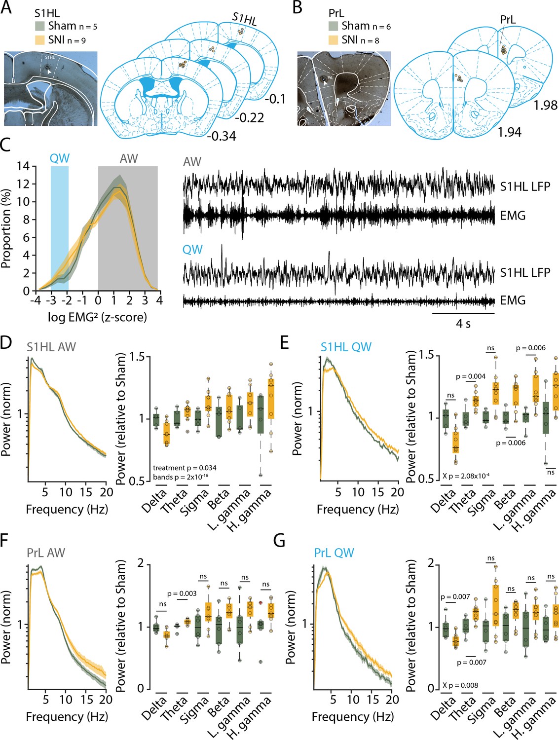
Three weeks after spared nerve injury (SNI), animals display alterations in the power spectra of quiet wakefulness within pain matrix areas.
(A, B) Histological verification of recording sites for S1 hindlimb cortex (S1HL) and prelimbic cortex (PrL). Left panel: representative brain section showing the lesion caused by postmortem electrocoagulation (arrowhead). Right panel: summary of all recording sites across animals (small circles). Anteroposterior stereotaxic coordinates relative to Bregma. (C) Histogram showing mean distributions of EMG power values (z-scored) during wakefulness for Sham and SNI. Shaded areas indicate values selected for quiet (QW) and active (AW) wakefulness. Representative traces for QW and AW shown on the right. (D, E) Left: log-scaled power spectrum density of S1HL local field potential (LFP) in AW (D) and QW (E) for Sham (n = 5) and SNI (n = 9) animals. Quantification of theta (5–10 Hz), beta (16–25 Hz), and the low gamma (26–40 Hz) frequency range. All data obtained from two successive light phases. For display, the mean level of the Sham for each band was set as 1. Statistics were done on log-transformed values extracted from the spectrum on the left. (F, G) Same as (D) and (E) for PrL LFP in AW (F) and QW (G) for Sham (n = 6) and SNI (n = 8) animals. For panel (F), Wilcoxon rank-sum tests were done. In this and all subsequent figures, significant main effects and interactions from the ANOVAs are given. Post-hoc tests were done once interactions were significant, with corresponding p values shown. For (D–G), X p denotes p value obtained from factorial interaction in the mixed-model ANOVAs, p values next to the data points derived from post-hoc tests. Corrected α = 0.0083.
-
Figure 2—source data 1
Source data for Figure 2C–G.
There is one .csv file for each panel. Additionally, a commented .pdf file with normality test, test statistics, and p values is provided.
- https://cdn.elifesciences.org/articles/65835/elife-65835-fig2-data1-v3.zip
Figure 3

Preserved sleep-wake behavior accompanied by pathological changes in sleep after spared nerve injury (SNI).
(A) Mean percentage of total time spent in the three main vigilance states for Sham (n = 18) and SNI (n = 18) animals in light (left) and dark phase (right) in baseline (B) and at day 20+ (D20+) after surgery. Black lines connect data from single animals. Mixed-model ANOVAS were applied. (B) Bout size cumulative distribution (with Kolmogorov–Smirnov [KS] test results) and time spent in short, intermediate, and long bouts for non-rapid eye movement sleep (NREMS) (left) and rapid eye movement sleep (REMS) (right) between Sham and SNI at D20+. Mixed-model ANOVA for time in bouts (a log transform for normality criteria was used for NREMS). (C) Mean latency to sleep onset. Mixed-model ANOVA, not significant (ns). (D) Number of microarousals (MAs) per hour of NREMS in light phase. Mixed-model ANOVA, ns. (E) Heart rate in NREMS (left) and REMS (right) from animals with suitable EMG signal, Sham (n = 17) and SNI (n = 14). Mixed-model ANOVA with three factors interaction followed by post-hoc tests. Corrected α = 0.0125. (F) Left: normalized power spectrum for Sham and SNI for NREMS at baseline and D20+. Shaded errors are 95% confidence intervals of the means. Right: high-gamma power (60–80 Hz) for D20+ relative to baseline (from the spectra shown on the left). One-sample t-tests with corrected α = 0.0167. (G) Same display as (F) for REMS. Spectra are presented up to 20 Hz to highlight the characteristic peaks for NREMS and REMS at low frequencies.
-
Figure 3—source data 1
Source data for Figure 3A–G.
For panels (A, C, D), two .csv files containing data from all three panels are provided for the light and the dark phase. For panel (B), six .csv files are provided for each dataset in the cumulative plots and the binned data for both non-rapid eye movement sleep (NREMS) and rapid eye movement sleep (REMS). One .csv file is provided for panel (E), whereas for panels (F, G), two .csv files are included separately for the power spectra at baseline and at D20+. One .csv file is provided for the gamma power analysis combining both NREMS and REMS. Additionally, a commented .pdf file with test statistics and p values is provided.
- https://cdn.elifesciences.org/articles/65835/elife-65835-fig3-data1-v3.zip
Figure 4

Preserved 0.02 Hz-fluctuation and phase-coupling to microarousals (MAs) three weeks after spared nerve injury (SNI).
(A, B) Representative traces of sigma power dynamics, with hypnograms shown below for W: wakefulness; N: non-rapid eye movement sleep (NREMS); R: rapid eye movement sleep (REMS). The circles represent the result of detection of individual cycles of the fluctuation, as described in Materials and methods. (C) Power in the infraslow range extracted from sigma power dynamics for Sham and SNI (n = 18 each); shaded areas represent 95% confidence intervals (CIs). (D) Number of infraslow cycles per hour of NREMS. Data are shown for D20+ only, but baseline data points were included in the statistical analysis. (E) Histograms of the phase values of the 0.02 Hz-fluctuation at MA onset for Sham and SNI, calculated as in Figure 1D. Vertical lines denote mean phase ± 95% CI for Sham: 152.3 ± 1.4; SNI: 150.4 ± 1.3. (F) Proportion of fragility periods (defined by 0.02 Hz-fluctuation phase values of 90–270°) containing an MA, continuing into NREMS or containing a transition to REMS. (G) Delta power dynamics across two light and dark phases and after a 6 hr sleep deprivation (SD). Rec: recovery period; Ctrl: control periods. Delta power values are normalized to the mean of those at ZT9-12. Shaded areas represent SEM. SD was carried out on a subset of 12 Sham and 12 animals with SNI on the day following the D20+ recording. (H) Boxplot for delta power values during Rec, corrected α = 0.0125. (I, J) As (G, H) for the number of MAs per hour of NREMS. (K, L) As (G, H), for the preferred phase of the 0.02 Hz-fluctuation at MA onset. In this figure, mixed-model ANOVAs followed by parametric post-hoc tests or nonparametric tests were used with corrected α = 0.0125.
-
Figure 4—source data 1
Source data for Figure 4C–L.
There is one .csv file for each panel. Additionally, a commented .pdf file with normality test, test statistics, and p values is provided.
- https://cdn.elifesciences.org/articles/65835/elife-65835-fig4-data1-v3.zip
Figure 5
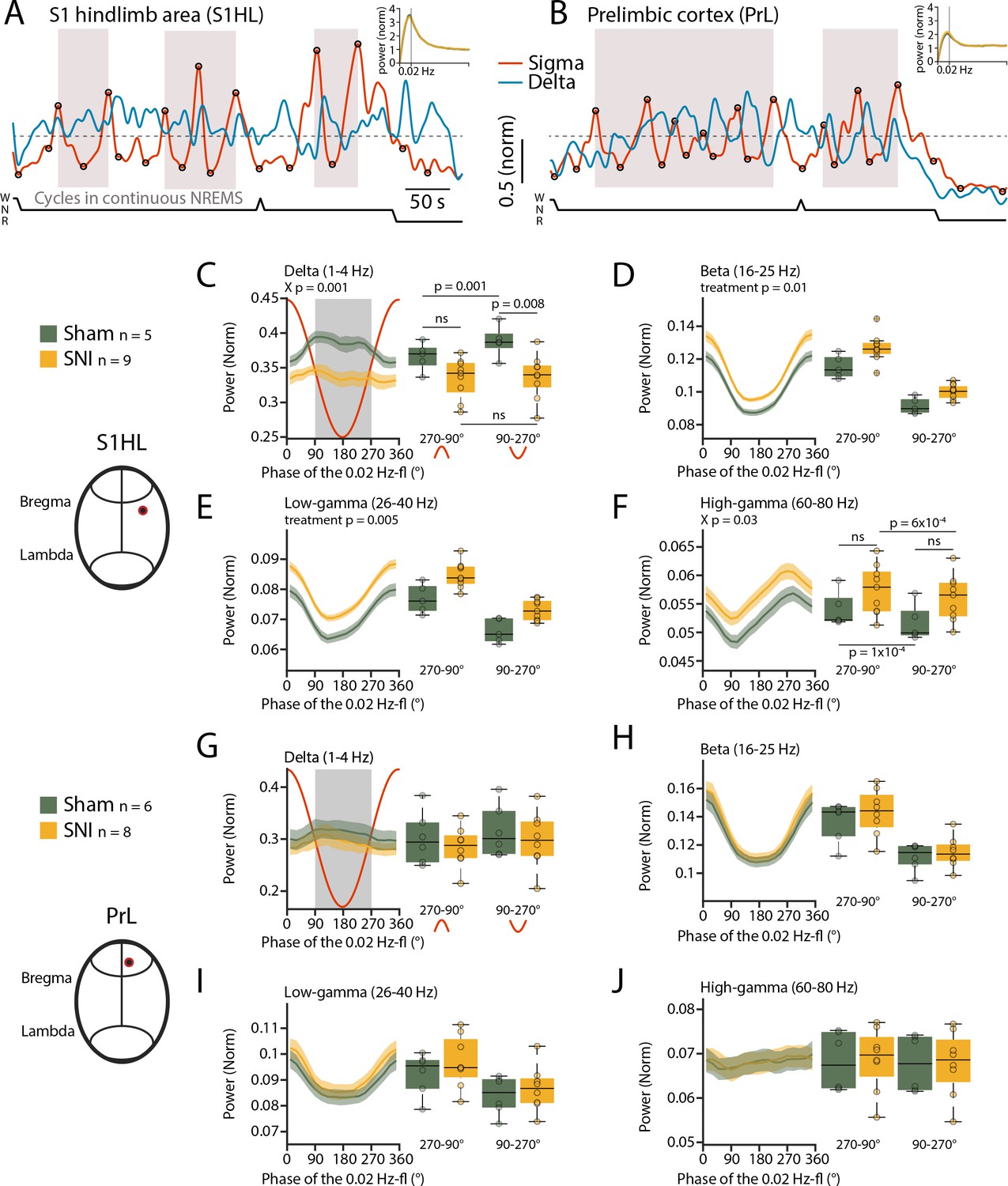
Spared nerve injury (SNI) induces locally disrupted spectral power dynamics during non-rapid eye movement sleep (NREMS).
(A, B) Sigma (10–15 Hz) and delta (1–4 Hz) dynamics during the same NREMS period in S1 hindlimb cortex (S1HL) (A) and prelimbic cortex (PrL) (B) during a baseline recording. Hypnograms shown below. Circles represent peaks and troughs used to detect the 0.02 Hz-fluctuation cycles (see Materials and methods). Shaded areas indicate 0.02 Hz-fluctuation cycles that are continuing uninterrupted in NREMS. Insets: power spectra of sigma power dynamics in the infraslow range. (C–F) For S1HL, trajectories of power in specific frequency bands across uninterrupted cycles of the 0.02 Hz-fluctuation, quantified in 20° bins. Red line shows the corresponding 0.02 Hz-fluctuation phase. Boxplots quantify spectral power within continuity (270–90°, red inverted U-shaped line) and fragility periods (90–270°, red U-shaped line). For all bands, mixed-model ANOVAs were done, followed by post-hoc t-tests if applicable. Significance for main effects and/or interaction (X p) is shown on top of the graphs, and post-hoc tests with corrected α = 0.0125 are presented next to the data. (G–J) Analogous presentation for PrL.
-
Figure 5—source data 1
Source data for Figure 5A–J.
There is one .csv file for each panel. Additionally, a commented .pdf file with normality test, test statistics, and p values is provided.
- https://cdn.elifesciences.org/articles/65835/elife-65835-fig5-data1-v3.zip
Figure 6 with 1 supplement
Mice generate local cortical arousals during non-rapid eye movement sleep (NREMS) that appear more frequently 3 weeks after spared nerve injury (SNI).
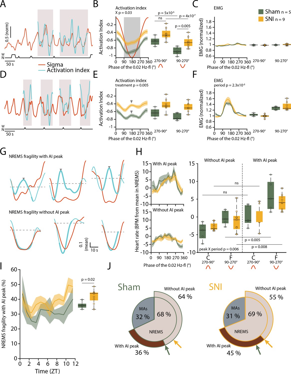
(A) Normalized dynamics of sigma power (10–15 Hz) and activation indices (calculated as the natural logarithm of (beta + low-gamma)/delta). Hypnogram is shown below. Shaded areas show cycles of the 0.02 Hz-fluctuation continuing into NREMS. (B) Activation indices (AIs) for cycles continuing into NREMS, with mean values shown in boxplots for continuity (270–90°) and fragility periods (90–270°). Mixed-model ANOVAs followed by post-hoc t-tests, corrected α = 0.0125. (C) Corresponding EMG values (normalized to the mean value in NREMS). Mixed-model ANOVA, ns: not significant. (D–F) Same as (A–C), for cycles of the 0.02 Hz-fluctuation associated with microarousals (MAs). Shaded areas in panel (D) show cycles of the 0.02 Hz-fluctuation interrupted by an MA. Arrowhead in (E) denotes the peak of the intermittent increase in AI due to MA occurrence. Mixed-model ANOVAs yielded single-factor effects. (G) Six individual cases in one Sham animal illustrating sigma (red) and AI (blue) dynamics in uninterrupted cycles of the 0.02 Hz-fluctuation. Thick portions of the blue traces represent the AI during the fragility period. Top and bottom three examples show an AI without and with an intermittent peak, respectively. The horizontal line (mean AI per cycle) represents the threshold for peak detection. (H) Left: heart rate dynamics for cycles continuing into NREMS. Cycles are divided into whether or not an AI peak was present. Right: boxplot quantification for continuity (C, 270–90°) and fragility periods (F, 90–270°), for Sham and SNI. Three-factor mixed-model ANOVAs followed by post-hoc t-tests, corrected α = 0.0125. (I) Occurrence of fragility periods with intermittent peak in AI across the light phase. Unpaired t-test. (J) Two level-pie plots for Sham (left) and SNI (right) representing the proportion of cycles containing an MA or continuing into NREMS. These latter fragility periods are further subdivided into the ones with intermittent peak (‘peak’) and without intermittent peak (‘no peak’). The arrows show the proportions for Sham (green) and SNI (yellow).
-
Figure 6—source data 1
Source data for Figure 6B,C,E,F,H,I.
There is one .csv file for each panel. Additionally, a commented .pdf file with normality test, test statistics, and p values is provided.
- https://cdn.elifesciences.org/articles/65835/elife-65835-fig6-data1-v3.zip
Figure 6—figure supplement 1
Activation index (AI) with peaks in fragility period in EEG and prelimbic cortex (PrL) local field potential (LFP) recordings.
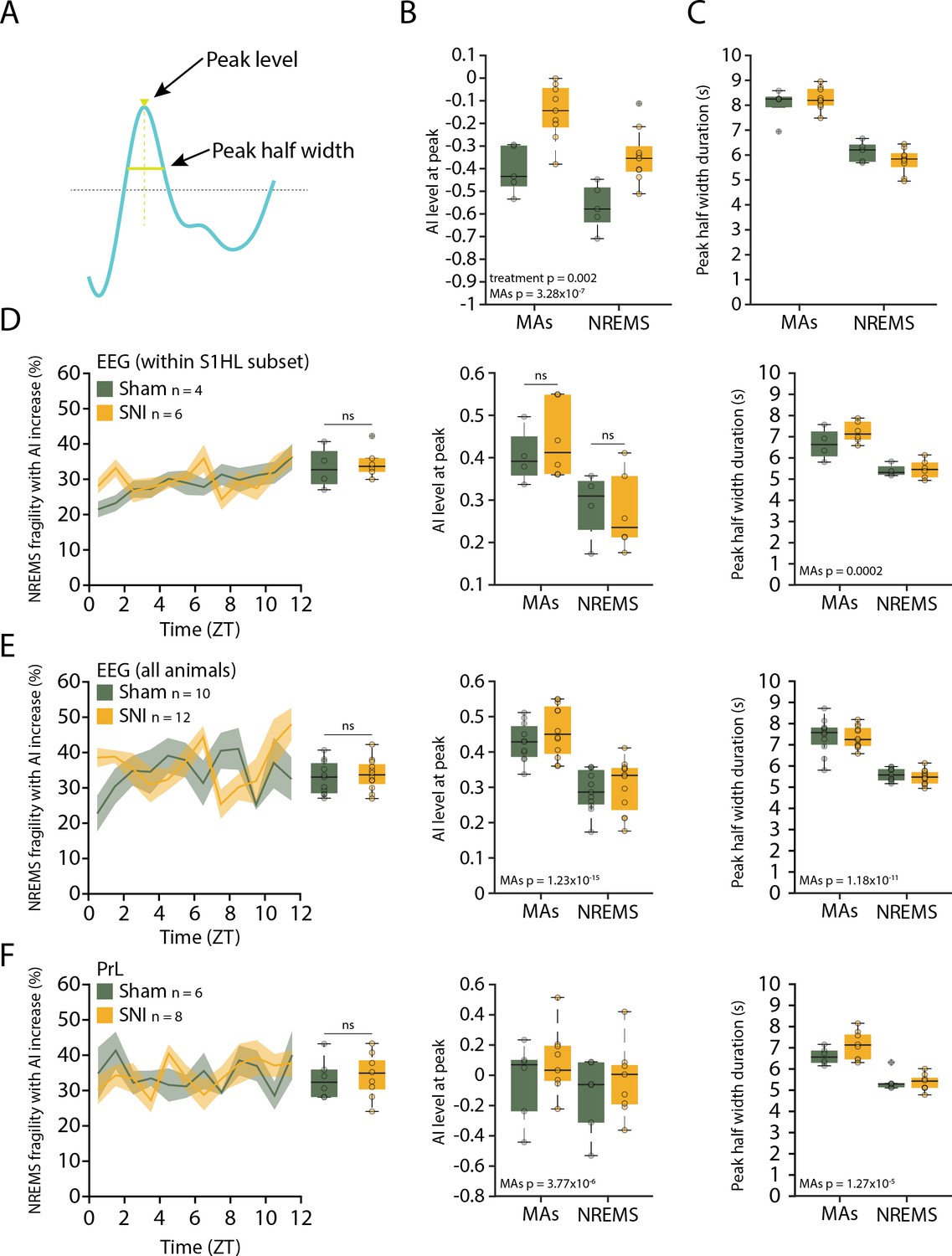
(A) Example of an AI peak, defining the parameters that were extracted for analysis. (B) Amplitudes for the AI peak detected in S1 Hindlimb cortex (S1HL) in Sham and spared nerve injury (SNI), with or without the presence of a microarousal (MA) in the fragility period. Significant p values for the factors in mixed-model ANOVAs indicated. (C) As (B), for the half-width of the AI peak. (D) Left: proportion of fragility periods containing an AI peak over the 12 hr light phase, detected in the frontoparietal EEG (contralateral to Sham or SNI surgeries) in the subset of animals from which the S1HL data were obtained in Figure 6. The data from one Sham and three animals with SNI were left out because the EEG was implanted ipsilateral to Sham or SNI surgeries. Middle: mean amplitude of the AI peaks in the EEG, in Sham and SNI. Corrected α = 0.0125. Right: half-width duration of the AI peaks in the EEG, with or without the presence of an MA in the fragility period. (E) Data from the frontoparietal EEG (contralateral to Sham or SNI surgeries) from all animals with combined EEG/EMG and LFP recordings. Same layout as in (D). (F) Data from PrL LFP recordings. Same layout as in (D) and (E). All statistics done with mixed-model ANOVAs followed by post-hoc t-tests, with the exception of panel (D), middle, for which Wilcoxon rank-sum tests were used.
-
Figure 6—figure supplement 1—source data 1
Source data for Figure 6—figure supplement 1B–F.
There is one .csv file for panels (B, C) and three each for all other panels for data corresponding to each graph. Additionally, a commented .pdf file with normality test, test statistics, and p values is provided.
- https://cdn.elifesciences.org/articles/65835/elife-65835-fig6-figsupp1-data1-v3.zip
Figure 7 with 1 supplement
Online detection of fragility periods during mouse non-rapid eye movement sleep (NREMS).
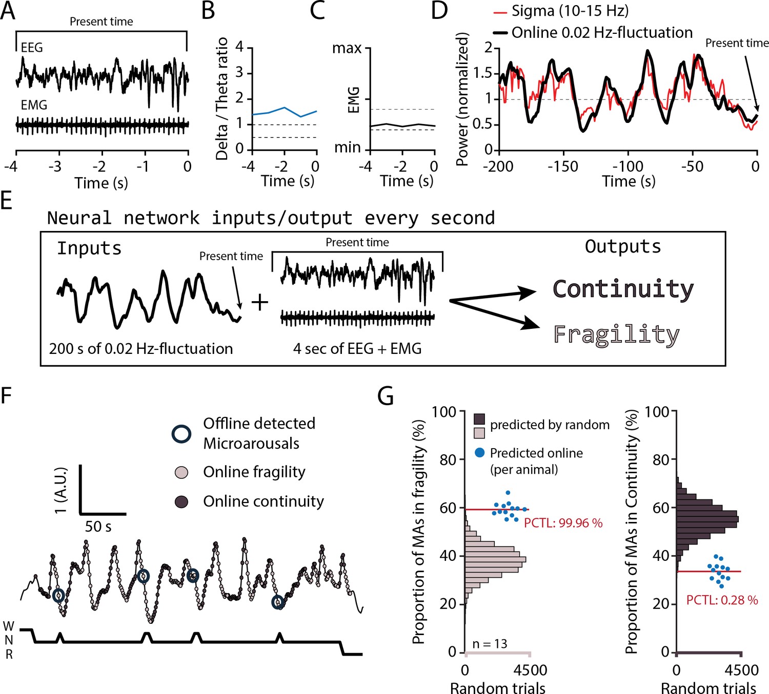
(A–E) Input and output parameters for machine learning of NREMS fragility and continuity periods. The network was trained to use the last 200 s of online 0.02 Hz-fluctuation and the present window of EEG and EMG values to determine whether the animal was in continuity or in fragility periods. (F) Representative result of an online detection of fragility (light gray circle) and continuity (dark gray circle) periods. The hypnogram below represents the visual scoring done offline, with detected microarousals (MAs) superimposed by open circles over the corresponding point of online detection. (G) Proportion of MAs scored during online-detected fragility (left) or continuity (right) for 13 animals (blue dots). Horizontal histograms represent the distribution of possible values of these proportions for randomly shuffled points of fragility or continuity. The mean proportions for the 13 animals fell at percentile (PCTL) 99.96% for fragility and 0.28% for continuity.
-
Figure 7—source data 1
Source data for Figure 7G.
Two .csv files are provided for the two datasets of the panel.
- https://cdn.elifesciences.org/articles/65835/elife-65835-fig7-data1-v3.zip
Figure 7—figure supplement 1
Online 0.02 Hz-fluctuation extraction and training of the neural network.
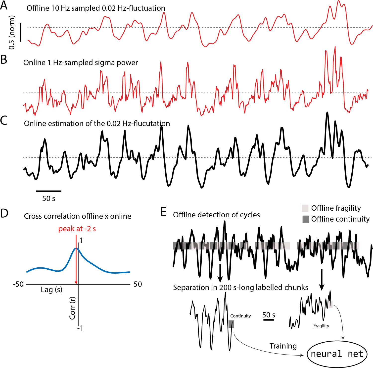
(A) 0.02 Hz-fluctuation from a non-rapid eye movement sleep (NREMS) period extracted offline as described in Figure 1—figure supplement 1. (B) Corresponding sigma power values collected online at 1 Hz. (C) Corresponding online-estimated 0.02 Hz-fluctuation, based on a ninth-order polynomial fit on the sigma values shown in (B). (D) Validation of the online estimate through cross-correlation with offline data from a 12 hr recording from one animal. The red arrow indicates the position of the highest correlation, showing a minor lag (–2 s). (E) Illustration of data labeling to train the neural network. The cycle detection (see Materials and methods) was used offline on the 0.02 Hz-fluctuation previously extracted online. Continuity was set to the ascending periods and fragility to the descending one. When conditions for complete cycles were not met, the label ‘none’ was applied. Then, 200 s-long chunks of this signal were extracted and labeled with continuity, fragility, or none depending on the position of the last point.
Figure 8 with 1 supplement
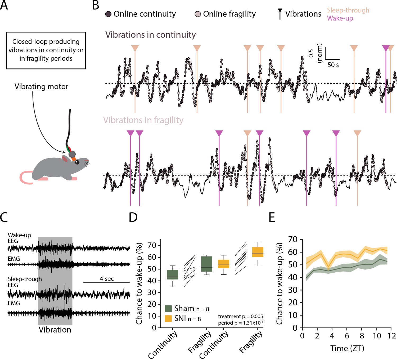
Spared nerve injury (SNI) induces higher somatosensory arousability.
(A) Experimental set-up. A small vibrating motor was fixed at the end of the recording cable that was connected to the animal’s headstage. Using the algorithm presented in Figure 7, a 3-s mild vibration (see Materials and methods) was delivered with a chance of 25% during either continuity or fragility periods. (B) Example experiments. Dark and light circles represent the online detection. Vertical lines represent the moments when the vibrations were delivered. Color codes for wake-ups or sleep-throughs. (C) Representative EEG/EMG recordings of a wake-up (top) and a sleep-through (bottom). Time of stimulus delivery is shaded. (D) Chances to wake-up in response to a vibration in online continuity or online fragility periods. A mixed-model ANOVA was done, yielding significant factor effects but no interaction. (E) Probability of wake-up (pooled continuity and fragility) for Sham and SNI over the light phase (ZT0-12). Shaded areas are SEMs.
-
Figure 8—source data 1
Source data for Figure 8D, E.
There is one .csv file for each panel. Additionally, a commented .pdf file with normality test, test statistics, and p values is provided.
- https://cdn.elifesciences.org/articles/65835/elife-65835-fig8-data1-v3.zip
Figure 8—figure supplement 1
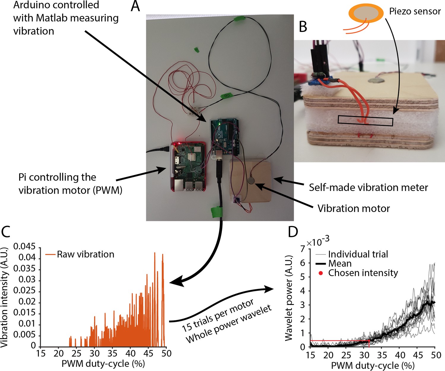
Vibration motor calibration for closed-loop somatosensory arousability testing.
(A) Photo overview of the calibration set-up, showing the vibration motor positioned onto a self-made piezometer containing the sensor (bottom right). The analog voltage generated by the sensor was measured by an Arduino and data fed into Matlab. To start vibrations, a Raspberry Pi sent a pulse-width modulation (PWM) signal to the vibration motor to modulate vibration intensity (achieved through increasing duty cycle from 15% to 50%). A TTL signal sent from the Raspberry Pi to the Arduino initiated the trial. (B) Close-up view of the self-made piezometer. The piezometer was composed of protective foam sandwiched and glued between two thin wooden plates. The upper plate contained a hole the size of the vibration motors and the lower one was fixed to the table using two-sided adhesive tape. The piezo sensor was inserted inside the foam part and a resistance (1000 Ohm) was used in the circuit. (C) Plot of data received from one vibration measurement trial. The vibration curve was calculated from each trial using whole-power wavelet transform. (D) Calibration curve (mean of 15 trials) used to find the necessary duty-cycle value. The chosen intensity was the same for all the motors.
Additional files
-
Supplementary file 1
Table for complete statistical information for all figure panels, arranged according to figure panel, statistical test used, group size, value of test statistics, p values, and Cohen’s effect sizes.
We have instead removed this info from all figure legends to simplify reading.
- https://cdn.elifesciences.org/articles/65835/elife-65835-supp1-v3.docx
-
Transparent reporting form
- https://cdn.elifesciences.org/articles/65835/elife-65835-transrepform1-v3.docx
-
Source code 1
Extraction of individual cycles of the 0.02 Hz-fluctuation.
- https://cdn.elifesciences.org/articles/65835/elife-65835-supp2-v3.zip
-
Source code 2
Analysis of transitions out of fragility periods, characterized by Hilbert angles from 90 to 270°.
- https://cdn.elifesciences.org/articles/65835/elife-65835-supp3-v3.zip
-
Source code 3
Hilbert phase analysis of the 0.02 Hz-fluctuation.
- https://cdn.elifesciences.org/articles/65835/elife-65835-supp4-v3.zip
-
Source code 4
Extraction of 0.02 Hz-fluctuation from one non-rapid eye movement sleep bout at 10 Hz resolution.
- https://cdn.elifesciences.org/articles/65835/elife-65835-supp5-v3.zip
-
Source code 5
Wavelet analysis used for calculation of sigma power dynamics, used in Source code 4.
- https://cdn.elifesciences.org/articles/65835/elife-65835-supp6-v3.zip
Download links
A two-part list of links to download the article, or parts of the article, in various formats.
Downloads (link to download the article as PDF)
Open citations (links to open the citations from this article in various online reference manager services)
Cite this article (links to download the citations from this article in formats compatible with various reference manager tools)
Cortico-autonomic local arousals and heightened somatosensory arousability during NREMS of mice in neuropathic pain
eLife 10:e65835.
https://doi.org/10.7554/eLife.65835


