Differential dopaminergic modulation of spontaneous cortico–subthalamic activity in Parkinson’s disease
- Institute of Clinical Neuroscience and Medical Psychology, Medical Faculty, Heinrich-Heine University Düsseldorf, Germany
- Department of Psychiatry, University of Oxford, United Kingdom
- Department of Clinical Health, Aarhus University, Denmark
- Department of Neurosurgery, University Hospital Düsseldorf, Germany
- Department of Neurology, Center for Movement Disorders and Neuromodulation, Medical Faculty, Heinrich-Heine University Düsseldorf, Germany
Figures
Figure 1
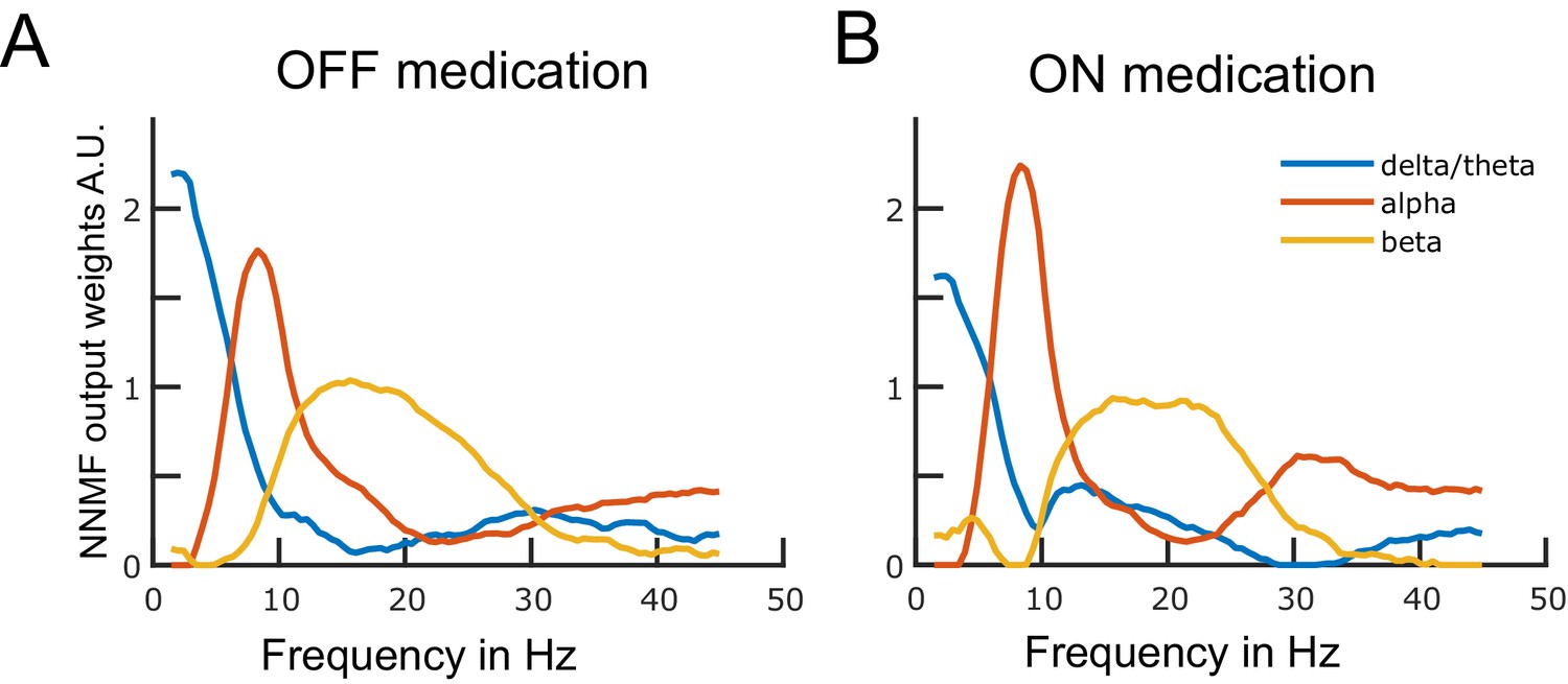
Data-driven frequency modes.
Each plotted curve shows a different spectral band. The x-axis represents frequency in Hz and the y-axis represents the weights obtained from the non-negative matrix factorisation (NNMF) in arbitrary units. The NNMF weights are like regression coefficients. The frequency resolution of the modes is 0.5 Hz. Panels A and B show the OFF and ON medication frequency modes, respectively. Source data are provided as Figure 1—source data 1–2.
-
Figure 1—source data 1
Source data of Figure 1a.
- https://cdn.elifesciences.org/articles/66057/elife-66057-fig1-data1-v1.mat
-
Figure 1—source data 2
Source data of Figure 1b.
- https://cdn.elifesciences.org/articles/66057/elife-66057-fig1-data2-v1.mat
Figure 2 with 1 supplement
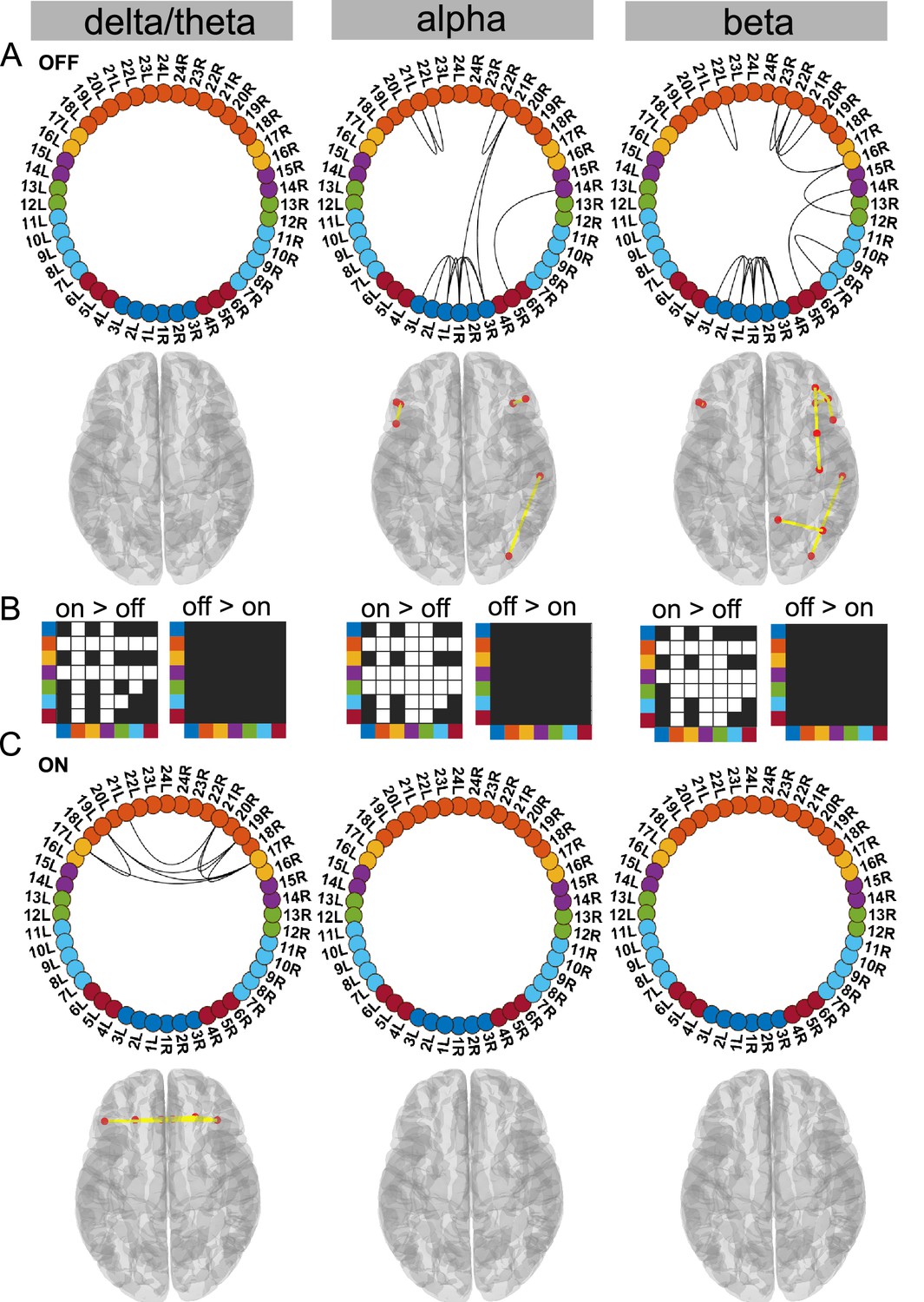
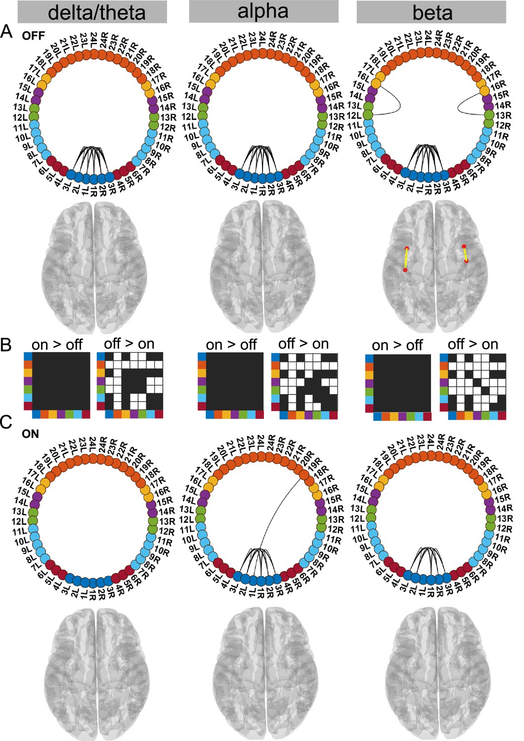
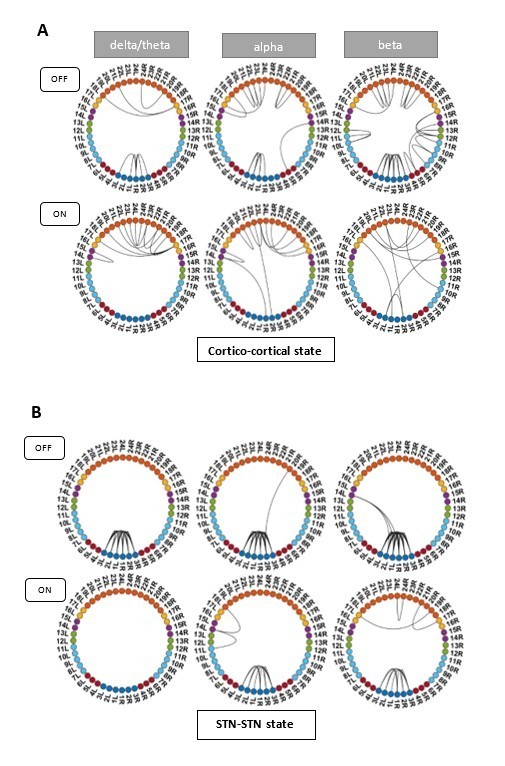
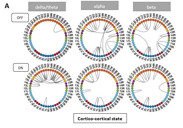
Cortico–cortical state.
The cortico–cortical state was characterised by a significant increase in coherence ON compared to OFF medication (see panel B). Due to this, no connections within the alpha and beta band ON medication were significantly higher than the mean (panel C). However, in the delta band, ON medication medial prefrontal–orbitofrontal connectivity emerged. (A and C) Each node in the circular graph represents a brain region based on the Mindboggle atlas. The regions from the atlas are listed in Table 1 along with their corresponding numbers that are used in the circular graph. The colour code in the circular graph represents a group of regions clustered according to the atlas (starting from node number 1) STN contacts (contacts 1, 2, 3 = right STN and contacts 4, 5, 6 = left STN), frontal, medial frontal, temporal, sensorimotor, parietal, and visual cortices. In the circular graph, only the significant connections (p<0.05; corrected for multiple comparisons, IntraMed analysis) are displayed as black curves connecting the nodes. The circles from left to right represent the delta/theta, alpha, and beta bands. Panel A shows results for OFF medication data and panel C for the ON medication condition. For every circular graph, we also show a corresponding top view of the brain with the connectivity represented by yellow lines and the red dot represents the anatomical seed vertex of the brain region. Only the cortical connections are shown. Panel B shows the result for inter-medication analysis (InterMed) for the cortico–cortical state. In each symmetric matrix, every row and column corresponds to a specific atlas cluster denoted by the dot colour on the side of the matrix. Each matrix entry is the result of the InterMed analysis where OFF medication connectivity between ith row and jth column was compared to the ON medication connectivity between the same connections. A cell is white if the comparison mentioned on top of the matrix (either ON >OFF or OFF >ON) was significant at a threshold of p<0.05. The connectivity maps of states 4–6 are provided in Figure 2—figure supplement 1. Source data are provided as Figure 2—source data 1–3.
-
Figure 2—source data 1
Source data of Figure 2a.
- https://cdn.elifesciences.org/articles/66057/elife-66057-fig2-data1-v1.mat
-
Figure 2—source data 2
Source data of Figure 2b.
- https://cdn.elifesciences.org/articles/66057/elife-66057-fig2-data2-v1.mat
-
Figure 2—source data 3
Source data of Figure 2c.
- https://cdn.elifesciences.org/articles/66057/elife-66057-fig2-data3-v1.mat
Figure 2—figure supplement 1
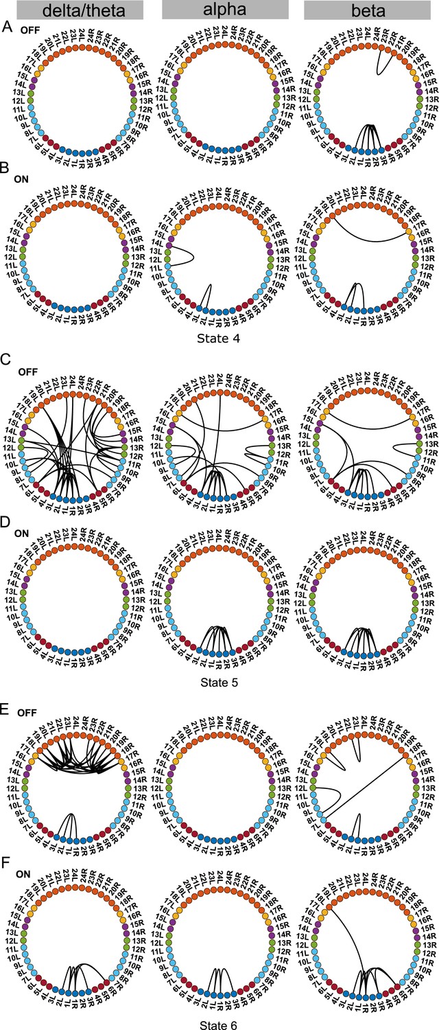
Three additional states that were found in the OFF and ON conditions.
Panels A, C, and E of each supplementary state are for the OFF medication condition. Panels B, D, and F are the distance-matched states ON medication. To the best of our knowledge, we could not interpret these states within our current physiological understanding of Parkinson’s disease.
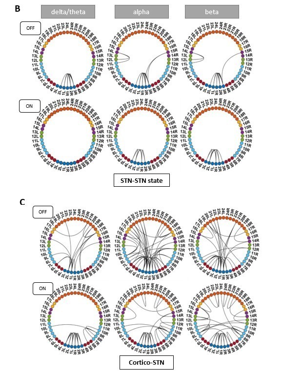
Figure 3
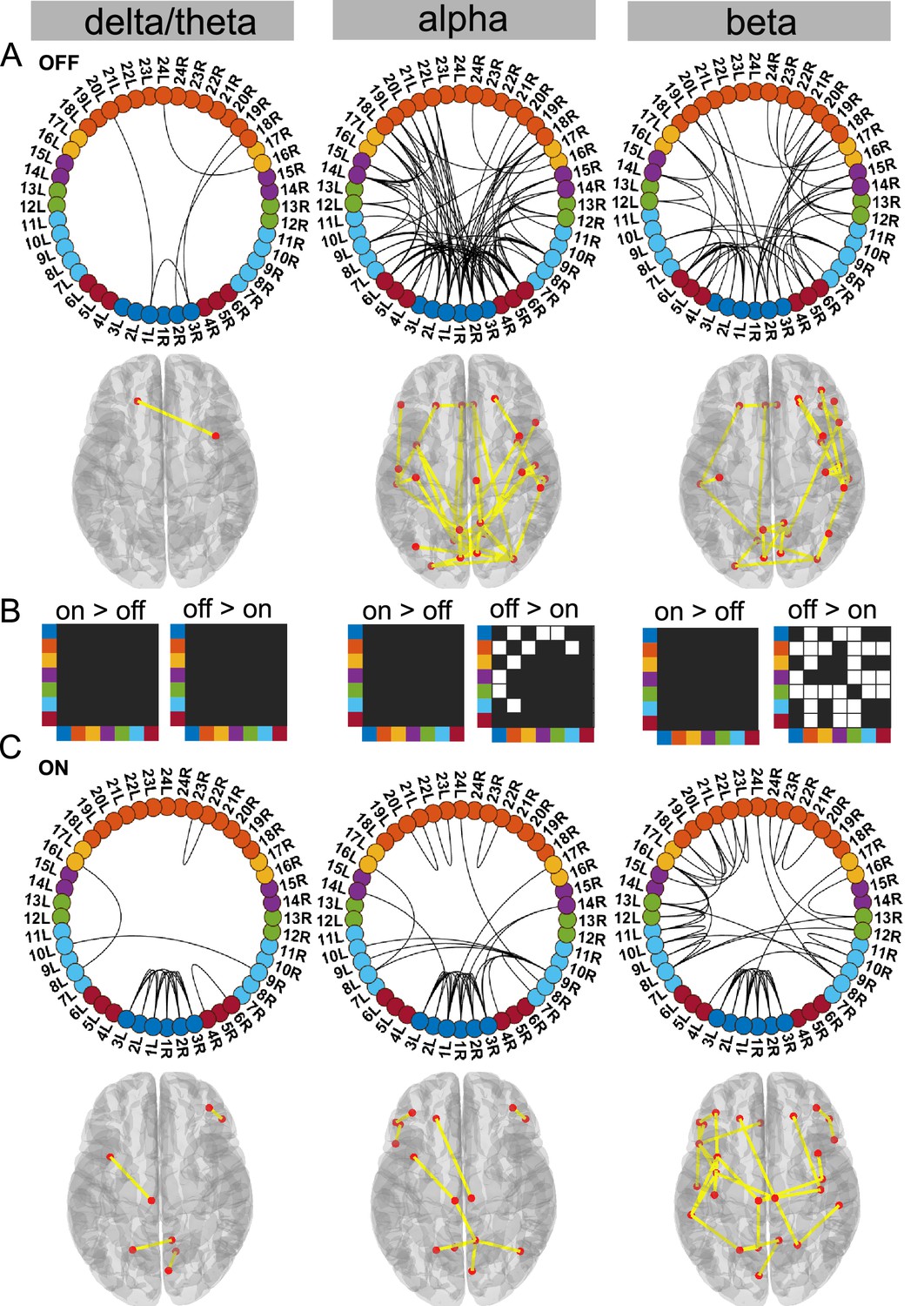
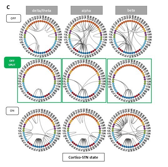
Cortico–STN state.
For the general description, see the note to Figure 2. The cortico–STN state was characterised by preservation of spectrally selective cortico–STN connectivity ON medication. Also, ON medication, a sensorimotor–frontoparietal network emerged. Source data are provided as Figure 3—source data 1–3.
-
Figure 3—source data 1
Source data of Figure 3a.
- https://cdn.elifesciences.org/articles/66057/elife-66057-fig3-data1-v1.mat
-
Figure 3—source data 2
Source data of Figure 3b.
- https://cdn.elifesciences.org/articles/66057/elife-66057-fig3-data2-v1.mat
-
Figure 3—source data 3
Source data of Figure 3c.
- https://cdn.elifesciences.org/articles/66057/elife-66057-fig3-data3-v1.mat
Figure 4
STN–STN state.
For the general description, see the note to Figure 2. The STN–STN state was characterised by preservation of STN–STN coherence in the alpha and beta band OFF versus ON medication. STN–STN theta/delta coherence was no longer significant ON medication. Source data are provided as Figure 4—source data 1–3.
-
Figure 4—source data 1
Source data of Figure 4a.
- https://cdn.elifesciences.org/articles/66057/elife-66057-fig4-data1-v1.mat
-
Figure 4—source data 2
Source data of Figure 4b.
- https://cdn.elifesciences.org/articles/66057/elife-66057-fig4-data2-v1.mat
-
Figure 4—source data 3
Source data of Figure 4c.
- https://cdn.elifesciences.org/articles/66057/elife-66057-fig4-data3-v1.mat
Figure 5
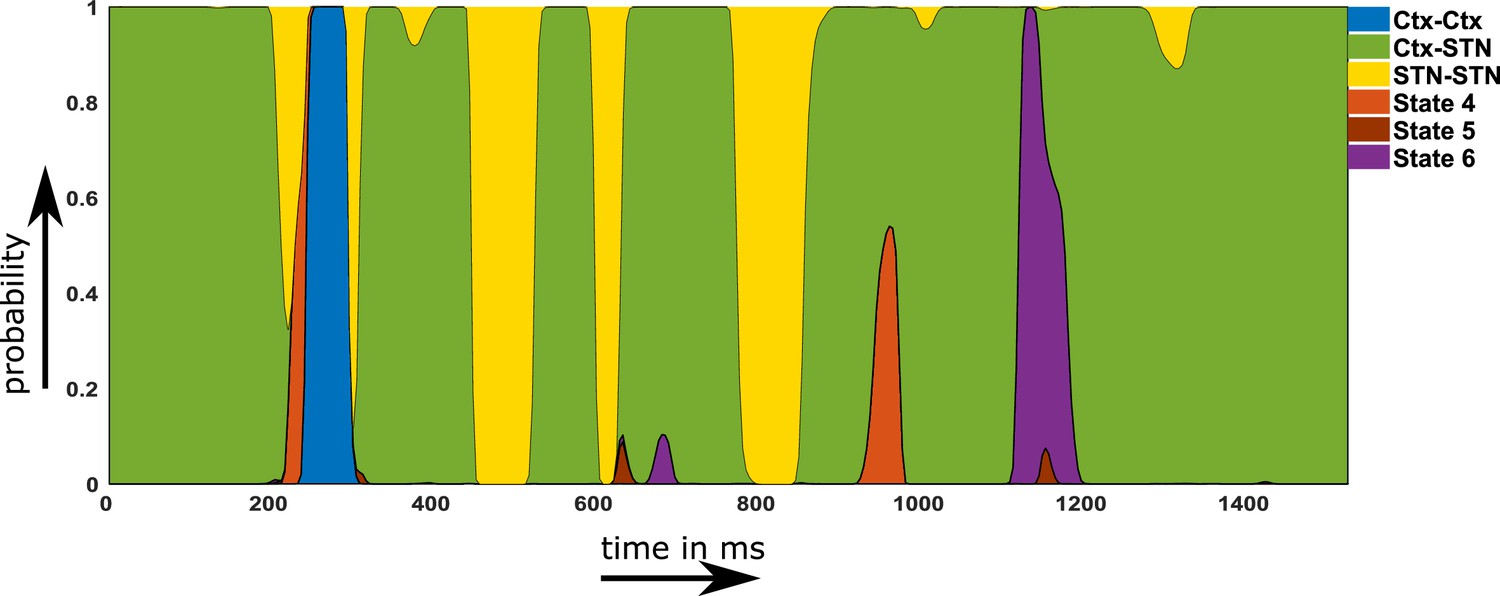
Example of a probability time course for the six hidden Markov model (HMM) states OFF medication.
Note that within the main text of the paper, we are only discussing the first three states. The connectivity maps of states 4–6 are provided in Figure 2—figure supplement 1. Source data are provided as Figure 5—source data 1–2.
-
Figure 5—source data 1
Probability time course first half in relation to Figure 5.
- https://cdn.elifesciences.org/articles/66057/elife-66057-fig5-data1-v1.mat
-
Figure 5—source data 2
Probability time course second half in relation to Figure 5.
- https://cdn.elifesciences.org/articles/66057/elife-66057-fig5-data2-v1.mat
Figure 6
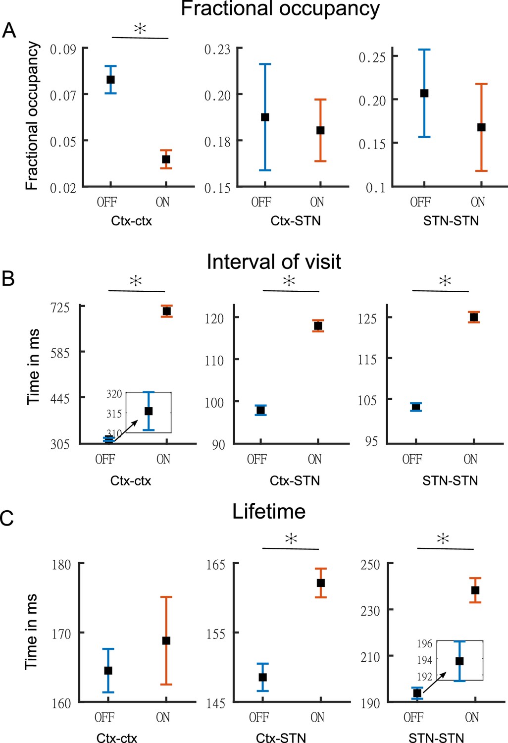
Temporal properties of states.
Panel A shows the fractional occupancy for the three states for the cortico–cortical (Ctx–Ctx), cortico–STN (Ctx–STN), and the STN–STN (STN–STN). Each point represents the mean for a state and the error bar represents standard error. Orange denotes ON medication data and blue OFF medication data. Panel B shows the mean interval of visits (in milliseconds) of the three states ON and OFF medication. Panel C shows the lifetime (in milliseconds) for the three states. Figure insets are used for clarity in case error bars are not clearly visible. The y-axis of each figure inset has the same units as the main figure. Source data are provided as Figure 6—source data 1–6.
-
Figure 6—source data 1
Source data of Figure 6a OFF medication.
- https://cdn.elifesciences.org/articles/66057/elife-66057-fig6-data1-v1.mat
-
Figure 6—source data 2
Source data of Figure 6a ON medication.
- https://cdn.elifesciences.org/articles/66057/elife-66057-fig6-data2-v1.mat
-
Figure 6—source data 3
Source data of Figure 6b OFF medication.
- https://cdn.elifesciences.org/articles/66057/elife-66057-fig6-data3-v1.mat
-
Figure 6—source data 4
Source data of Figure 6b ON medication.
- https://cdn.elifesciences.org/articles/66057/elife-66057-fig6-data4-v1.mat
-
Figure 6—source data 5
Source data of Figure 6c OFF medication.
- https://cdn.elifesciences.org/articles/66057/elife-66057-fig6-data5-v1.mat
-
Figure 6—source data 6
Source data of Figure 6c ON medication.
- https://cdn.elifesciences.org/articles/66057/elife-66057-fig6-data6-v1.mat
Figure 7
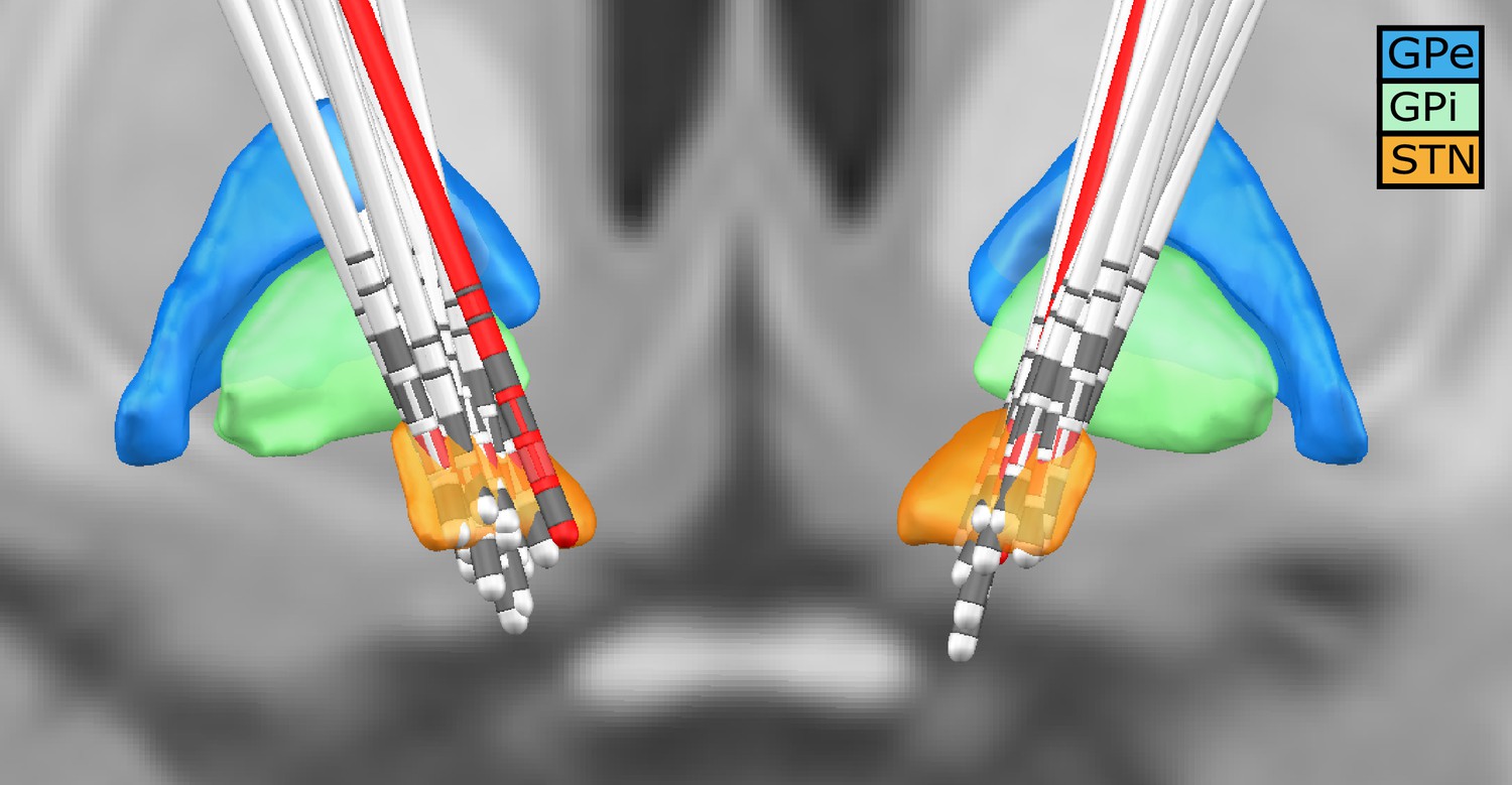
Deep brain stimulation (DBS) electrode location for all subjects.
Lead-DBS reconstruction with all subjects. The red leads are the ones of a subject with one of the outside the STN. The red directional contacts are the ones from which the data was used for analysis.
Author response image 1
States obtained after removing one tremor dominant and one mixed type patient from analysis.
Author response image 2
States obtained after removing one tremor dominant and one mixed type patient from analysis.
Panel C shows the split OFF medication cortico-STN state. Most of the cortico-STN connectivity is captured by the state shown in the top row (Figure 1 C OFF). Only the motor-STN connectivity in the α and β band (along with a medial frontal-STN connection in the α band) is captured separately by the states labeled “OFF Split” (Figure 1 C OFF SPLIT).
Author response image 3
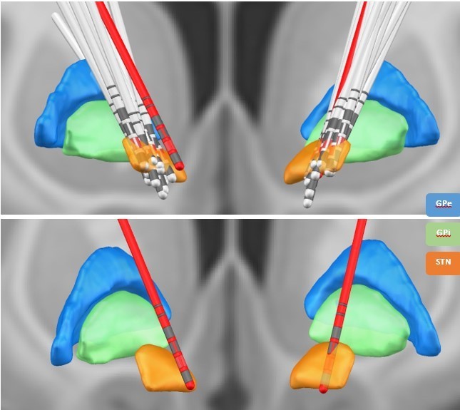
Lead DBS reconstruction of the location of electrodes in the STN for different subjects.
The red electrodes have not been placed properly in the STN. The contacts marked in red represent the directional contacts from which the data was used for analysis.
Author response image 4
HMM states obtained after running the analysis without the subject with the electrode outside the STN.
Author response image 5
HMM states obtained after running the analysis without the subject with the electrode outside the STN.
Tables
Table 1
Regions of the Mindboggle atlas used.
STN, subthalamic nucleus; Vis, visual; Par, parietal; Smtr, sensory motor; Tmp, temporal; Mpf, medial prefrontal; Frnt, frontal; Ctx, cortex. The colour code is for the ring figures presented as part of the results.
| STN | 1 | Contact one right | Smtr-Ctx | 12 | Postcentral |
|---|---|---|---|---|---|
| 2 | Contact two right | 13 | Precentral | ||
| 3 | Contact three right | Tmp-Ctx | 14 | Middle temporal | |
| 1 | Contact four left | 15 | Superior temporal | ||
| 2 | Contact five left | Mpf-Ctx | 16 | Caudal middle frontal | |
| 3 | Contact six left | 17 | Medial orbitofrontal | ||
| Vis-Ctx | 4 | Cuneus | Frnt-Ctx | 18 | Insula |
| 5 | Lateral occipital | 19 | Lateral orbitofrontal | ||
| 6 | Lingual | 20 | Pars opercularis | ||
| Par-Ctx | 7 | Inferior parietal | 21 | Pars orbitalis | |
| 8 | Para central | 22 | Pars triangularis | ||
| 9 | Precuneus | 23 | Rostral middlefrontal | ||
| 10 | Superior parietal | 24 | Superior frontal | ||
| 11 | Supramarginal |
Additional files
Download links
A two-part list of links to download the article, or parts of the article, in various formats.
Downloads (link to download the article as PDF)
Open citations (links to open the citations from this article in various online reference manager services)
Cite this article (links to download the citations from this article in formats compatible with various reference manager tools)
Differential dopaminergic modulation of spontaneous cortico–subthalamic activity in Parkinson’s disease
eLife 10:e66057.
https://doi.org/10.7554/eLife.66057


