Fully autonomous mouse behavioral and optogenetic experiments in home-cage
- Department of Neuroscience, Baylor College of Medicine, United States
Figures
Figure 1 with 1 supplement
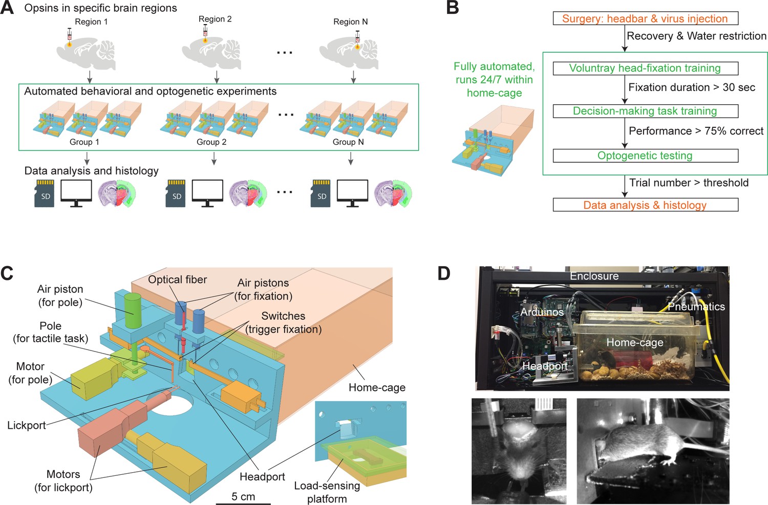
Workflow for autonomous behavior and optogenetic experiments and design of home-cage system.
(A) Workflow for autonomous behavioral and optogenetic experiments. In each group of mice, optogenetic opsins are expressed in a specific brain region. Naive mice undergo autonomous behavioral training and optogenetic testing in their home-cage. Multiple groups of mice are tested in parallel to examine multiple brain regions. Data is stored on SD cards for analysis. Histology is performed at the end of the workflow to register the targeted brain regions to an atlas. Green bounding box highlights the portion of the workflow that is unsupervised by experimenters. (B) Workflow for automated behavioral training and optogenetic testing. After recovery from surgery, mice are housed in the home-cage system 24/7. Automated computer algorithms train mice to perform voluntary head-fixation, decision-making task, and carry out optogenetic testing. The progression in the workflow is based on behavioral performance. Green bounding box corresponds to the bounding box in (A). (C) Design of the home-cage system. The main component is a behavioral test chamber which can be accessed through a headport from the home-cage. Inset shows the view of the headport from inside the home-cage. Mice access the headport on a load-sensing platform. See Figure 1—figure supplement 1 and Materialsand methods for details. (D) Photographs of the home-cage system. Top: side view of the system. The system is standalone with controllers (Arduinos) and actuators packed into a self-contained enclosure. Bottom, the front and back view of a mouse accessing the headport and performing the tactile decision task.
Figure 1—figure supplement 1
Overview of the home-cage system.
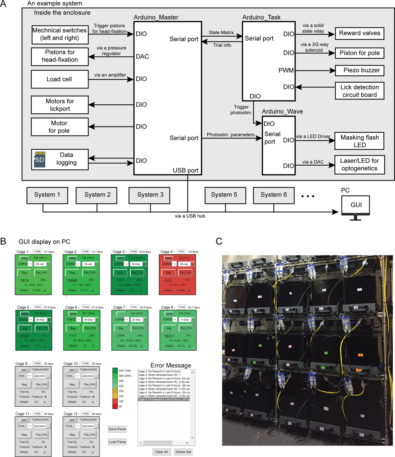
(A) Diagram of the control system for the home-cage system. The main controller consists of three Arduinos (‘Arduino Master’, ‘Arduino Task’, and ‘Arduino Wave’) that control peripherals through digital input/output (DIO), digital-analog-convertor (DAC), pulse width modulation (PWM) and serial ports. The ‘Master’ controllers from multiple systems can be connected to a PC to display mouse behavioral data in a GUI. See Materials and methods for details. (B) Screenshot of the GUI display. Each square shows one home-cage system. The color indicates the number of trials the mouse performed in the last 24 hr (ranging from green, >640 trials, to red, <80 trials). Gray squares are not connected to any system. Each square displays mouse meta data and behavioral training data, including mouse ID, body weight, training start date, days and number of trials performed since the start, number of trials performed in the last 24 hr, performance in the last 100 trials, and training protocol number. The two buttons labeled ‘Msg’ and ‘plot_p/w’ bring up additional windows to display messages from the home-cage system and plot detailed behavioral data from the last 24 hr. Error messages are also displayed in the bottom right box. (C) Fifteen standalone home-cage systems placed on a standard rack.
Figure 2 with 1 supplement

Voluntary head-fixation in home-cage.
(A) Left, schematic drawing of the custom headbar. Right, photograph of a headbar implant. (B) Schematic drawings of a head-fixation and release sequence. Headbar enters a widened track on both sides of the headport that guides the headbar into a narrow spacing at the end. Two mechanical switches located on either side of the headport trigger pneumatic pistons to clamp the headbar. Head-fixations are released by retracting the pneumatic pistons. (C) Left, photograph of the load-sensing platform with top plate removed and load cell exposed. Right, example readings from the load cell (20 samples/s) in a 24-hr period. Shaded areas, dark cycles. Absence of samples indicates the mouse is off the platform. The histogram shows all readings from the 24-hr period. The peak can be used to estimate the mouse’s body weight. (D) Example readings from the load cell during four consecutive head-fixations (green shades). Head-fixations typically reduce weight on the platform. Readings crossing a threshold (blue dashed line) result in self-release (blue arrows). Otherwise, the mouse is released after a predefined fixation duration (time-up release, green arrows). Fixation duration is 30 s in this example. (E) Flow chart of the head-fixation training protocol. See Materials and methods for details. (F) Data from an example mouse undergoing head-fixation training. Top, data from the first 4 days. The plots show lickport position (top, large value indicates further away from the home-cage, see inset), switch trigger events (middle), and head-fixation events (bottom). For head-fixation events, each tick indicates one fixation, with the height indicating fixation duration. The color indicates time-up release (green) and self-release (blue). Shaded areas, dark cycles. Time spent in learning headport entry and learning head-fixation are colored as in (E). Bottom: head-fixation data from the same mouse over 29 days. (G) Head-fixation duration over 40 days. Gray lines, individual mice; black line, mean. Bar plot shows average fixation duration throughout the entire head-fixation training. Error bar, standard deviation. Circles, individual mice. (H) Same as (G) but for mice without the self-release mechanism. (I) Displacement of the headbar implant across different head-fixations along medial-lateral, rostral-caudal, and dorsal-ventral directions. (J) Fraction of head-fixations in which mice trigger self-release. Gray line, individual mice; black line, mean. Bar plot shows average fraction throughout the entire head-fixation training. Error bar, standard deviation. Circles, individual mice. (K) Frequency of head-fixation across dark and light cycles. Bars show average across all mice. Error bars, standard deviations. (L) Time interval between head-fixations. Data from all mice are pooled.
Figure 2—figure supplement 1
Displacement of headbar implant across multiple head-fixations.
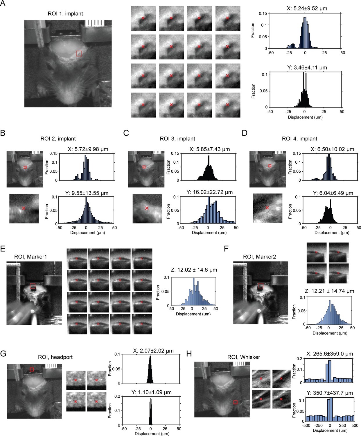
(A) Left, a region of interest (ROI) on the clear skull implant is indicated by the red bounding box (30 × 30 pixels). Middle, example frames within the ROI from 16 different head-fixations. Red cross indicates the center of mass based on pixel intensity. Right, histogram of displacement in the medial-lateral (x) and rostral-caudal (y) directions, calculated by sub-pixel correlations of ROIs across all possible pairs of frames from different head-fixations (Materials and methods). (B–D) Same as (A) for three other ROIs selected around the clear skull implant. (E–F) Same as (A) but for 2 ROIs around a marker attached to the skull to measure displacements in the dorsal-ventral direction (z). (G) Same as (A) but for a ROI on the wall above the headport. As expected, the ROI shows little displacement compared to (A)-(F). (H) Same as (A) but for a ROI on the mouse whiskers. As expected, the ROI shows large displacement compared to (A)-(F).
Figure 3 with 1 supplement
Tactile decision task in home-cage.
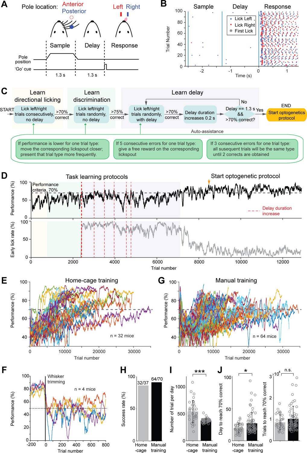
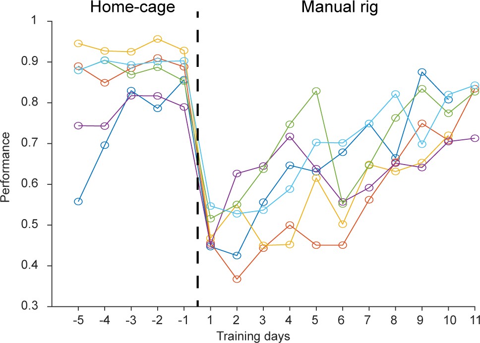
(A) Task structure. Mice discriminate the location of a pole (anterior or posterior) during a sample epoch (1.3 s) and report the location using directional licking (left or right) after a delay epoch (1.3 s). An auditory go cue (0.1 s) signals the beginning of the response epoch. (B) Example behavioral data in 100 consecutive trials. Dots show individual licks. Blue, lick right; red, lick left. Circles indicate the first lick after the go cue (choice). In trials with early licks before the ‘go’ cue, choice licks occur late due to the timeouts (Materials and methods). (C) Flow chart of the task training protocol. See Materials and methods for details. Auto-assist programs (green box) evaluate mice performance continuously and assist mice whenever certain behavioral biases are detected. (D) Data from an example mouse undergoing task training in home-cage. Top, behavioral performance. Shaded areas indicate different phases of the training as in (C). During the delay epoch training, the red dash lines indicate delay duration increases. Bottom, fraction of trials in which the mouse licked before the go cue. After mice complete the task training protocol, experimenters examine the mice performance and initiate optogenetic testing protocol (indicated by the orange arrow in this example). (E) Behavioral performance of all mice in home-cage training (n = 32). Black dash line, criterion performance, 70% correct. (F) In a subset of mice (n = 4), the right whiskers were trimmed after home-cage training. Behavioral performance dropped to chance level (50%, black dash line) and did not recover. (G) Behavioral performance of all mice in manual training (n = 64). (H) Percentage of mice successfully trained in home-cage vs. manual training. Training is deemed successful if the mouse reached 70% correct criterion performance. (I) Number of trials performed per day in home-cage versus manual training. Bar plot shows mean and standard deviation across mice. Circles, individual mice. ***, p<0.001, two-tailed t-test. (J) Left, number of days to reach 70% correct criterion performance. Right, number of trials to reach 70% correct criterion performance. *, p<0.05; n.s., p>0.05, two-tailed t-test.
Figure 3—figure supplement 1
Behavioral performance of home-cage trained mice after transferring to an electrophysiology setup.
After reaching high levels of performance in home-cage training, mice were transferred to an electrophysiology setup (day 0, dash line). Performance initially dropped but gradually recovered over 7 days as the mice acclimated to the new setup. The acclimation time is much less than the time needed to manually train naïve mice to perform the task (Figure 3). Thus, the automated home-cage system can train mice to support neurophysiology experiments. Individual lines show individual mice (n = 6).
Figure 4
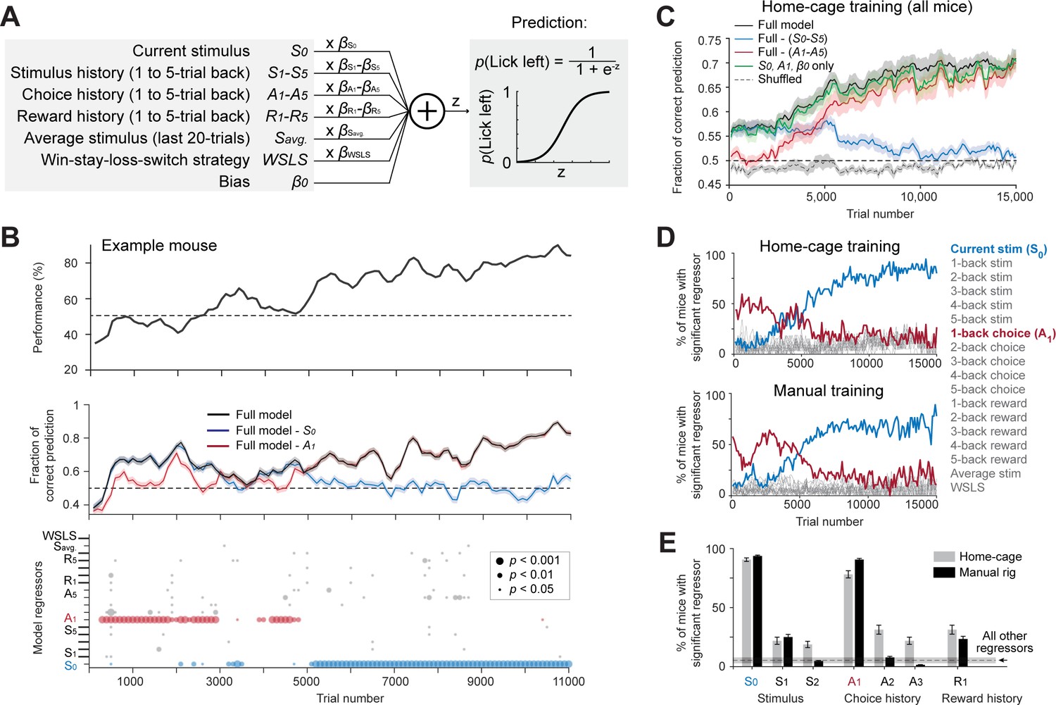
Model-based comparison of task learning in home-cage and manual training.
(A) A logistic regression model to predict choice. Weighted sum of the tactile stimulus, stimulus history, choice history, reward history, a win-stay-lose-switch strategy (choice x reward in the last trial), and a constant bias is passed through a logistic function to predict choice in the current trial. (B) Behavioral data and model prediction from an example mouse in home-cage training. Trials are binned (bin size, 500 trials; step size, 100 trials). Top, behavioral performance. Middle, prediction performance of the full model and two partial models excluding either the current stimulus (S0, blue) or 1-back choice (A1, red). Model performance is calculated as the fraction of choice predicted (Materials and methods; chance level is 50%). Shaded area indicates SEM. Bottom, the significance of individual regressors. Circle size corresponds to p values. The significance of a regressor is evaluated by comparing the prediction of the full model to a partial model with the regressor of interest excluded. p Values are based on bootstrap (Materials and methods). (C) Average model prediction across all mice in home-cage training. Black line, prediction of the full model. Blue, performance of a partial model excluding both the current stimulus S0 and stimulus history S1-5. Red, performance of a partial model excluding choice history A1-5. Green, performance of a partial model with only the current stimulus S0, choice history A1, and a constant bias term β0. Dashed line, the performance of the full model predicting shuffled behavioral data (Materials and methods). Shaded area indicates SEM across mice. Chance, 50%. (D) Percentage of mice showing significant contribution from each regressor at different stages of learning. Significance is defined as p<0.05. Top, mice in home-cage training (n = 32); Bottom, mice in manual training (n = 64). (E) Percentage of mice relying on different regressors during task learning. A mouse is deemed to rely on a regressor if it shows significant contribution to choice prediction in at least five consecutive time bins during training (1000 trials). Regressors shown are the current stimulus (S0), 1-back and 2-back stimulus history (S1-2), 1-back, 2-back and 3-back choice history (A1-3), and 1-back reward history (R1). Error bars show SEM across mice (bootstrap). Dash line and shaded area show the mean and SEM across all other regressors. All other regressors show small contributions and they are pooled. Regressors from both home-cage and manual training are also pooled.
Figure 5
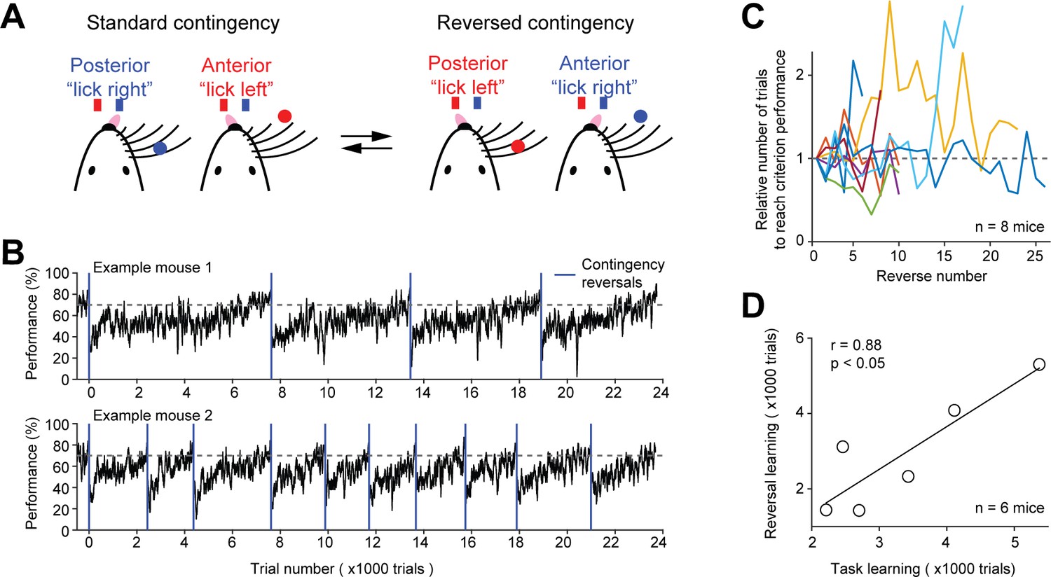
Contingency reversal learning in home-cage.
(A) Mice discriminate the location of a pole (anterior or posterior) and report the location using directional licking (left or right) without a delay epoch. The task switches between standard sensorimotor contingency and reversed contingency once mice reach criterion performance. Criterion performance, >80% for 100 trials. (B) Behavioral performance data from two example mice. Bin size, 50 trials. Blue line, contingency reversals. Dashed line, 70% correct. (C) The number of trials to acquire new contingencies over multiple contingency reversals. The number of trials to reach criterion performance is normalized to the first contingency reversal. Individual lines show individual mice. (D) The number of trials needed to learn the tactile decision task vs. the average number of trials to reach criterion performance in contingency reversal learning. Task learning is from the start of head-fixation training to reaching criterion performance. Individual dots show individual mice. Line, linear regression. Two mice from (C) were excluded because they previously learned a different behavioral task.
Figure 6
Contingency reversal learning in home-cage.
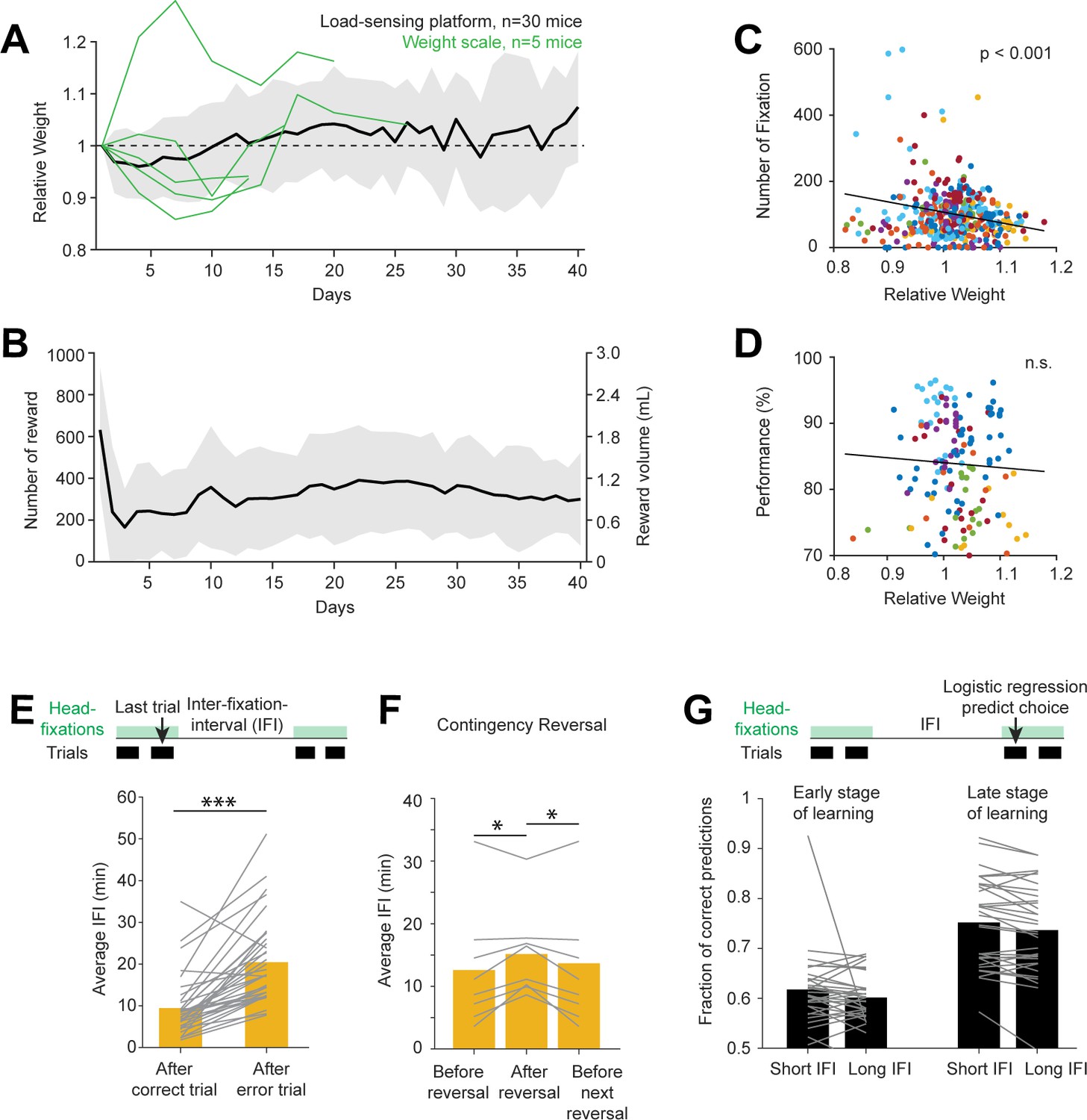
(A) Mouse weight as a function of time. Body weights were estimated from the load-sensing platform in home-cage (see Figure 2C). Weights are normalized to the initial weights on day 1. Black line and shades, mean ± standard deviation across mice. Green lines, in a subset of mice, body weights were also measured outside of the home-cage on a weight scale. (B) Number of rewards and water consumed per day. Line and shades, mean ± standard deviation across mice. (C) Number of head-fixations per day as a function of normalized body weights. Each symbol corresponds to one day. Different colors show different mice. (D) Task performance as a function of normalized body weights. Multiple factors can affect task performance, including motivation and task learning. Here, the data are taken from days after the mice have reached criterion performance. (E) Average IFI durations following correct and error trials. Individual lines show individual mice. Bars show averages across mice. ***p<0.001, paired two-tailed t-test. (F) Average IFI durations during contingency reversal learning. Trials are taken from periods right before contingency reversals, immediately following reversals, and before the next reversals. Individual lines show individual mice. Bars show averages across mice. *p<0.05, paired two-tailed t-test. (G) Prediction of choice by logistic regression on trials following long vs. short inter-fixation-intervals. The logistic regression model was fit using trials in their natural sequential order (regardless of the inter-fixation-intervals). The model was then used to predict choice on independent trials. Trials were then sorted by the preceding inter-fixation-intervals. Prediction performance was calculated separately for trials following short or long inter-fixation-intervals. Individual lines show individual mice. Bars show averages across mice. n.s. p>0.05, paired two-tailed t-test. (H).
Figure 7 with 2 supplements
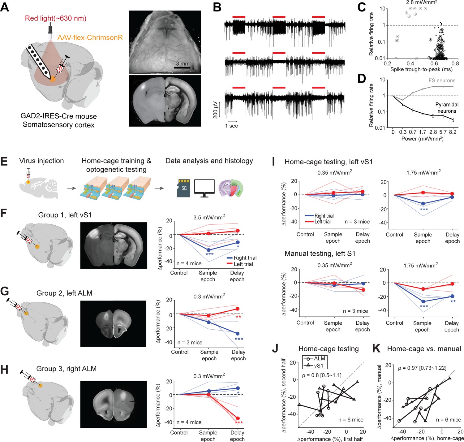
Photoinhibition of cortical regions and comparisons of home-cage optogenetic experiments with manual optogenetic experiments.
(A) Left, an optogenetic approach to silence activity in specific brain regions and electrophysiology characterization in the barrel cortex (vS1). Right top, an example clear skull implant. Right bottom, a coronal section showing ChrimsonR expression in vS1. The coronal section is aligned to the Allen Refence Brain (Materials and methods). (B) Silicon probe recording in vS1 during photostimulation. Multi-unit activity from three example channels showing photoexcitation (first row) and photoinhibition (second and third rows). Red lines, photostimulation. (C) Effects of photostimulation on cell types defined by spike waveform. Dots, individual neurons. Circled dots, neurons with significant spike rate change, p<0.05, two-tailed t-test. Spike rate of each neuron during photostimulation is normalized to its baseline (‘relative firing rate’, Materials and methods). Neurons with narrow spike waveforms are putative fast-spiking (FS) interneurons (gray). Neurons with wide spike waveforms are putative pyramidal neurons (black). (D) Relative firing rate of putative pyramidal neurons (black) and interneurons (gray) as a function of photostimulation intensity. Error bars show SEM across neurons. (E) Workflow schematics. (F) Photoinhibition of the left vS1. Left, a 3D rendered brain showing virus injection location. Middle, a coronal section showing virus expression in the left vS1. Right, behavioral performance change relative to the control trials during photoinhibition in the sample and delay epoch. Performance for lick left (red) and lick right trials (blue) are computed separately. Thin lines, individual mice; thick lines, mean. *p<0.025; **p<0.01; ***p<0.001, significant performance change compared to the control trials (bootstrap, Materials and methods). (G) Same as (F) but for photoinhibition of the left ALM. (H) Same as (F) but for photoinhibition of the right ALM. (I) Behavioral performance change relative to the control trials during photoinhibition in home-cage optogenetic experiments (top row) and manual optogenetic experiments (bottom row). See the full dose response in Figure 7—figure supplement 2. (J) Comparison of performance change during the first vs. second half of optogenetic testing. Data from all mice and experiments (left vS1 photoinhibition, three mice; left ALM photoinhibition, one mouse; right ALM photoinhibition, two mice). Lines connect data from multiple photostimulation intensities for individual mice. For each brain region, only the condition in which photoinhibition induced the largest behavioral effect is included. Left vS1, data from the lick right trials, sample epoch photoinhibition. Left ALM, data from the lick right trials, delay epoch photoinhibition. Right ALM, data from the lick left trials, delay epoch photoinhibition. Linear regression, slope: 0.8; range: 0.5–1.1 (95% confidential interval). There is no difference between the first and second half of the home-cage optogenetic experiments (p=0.78, paired t-test). Home-cage optogenetic experiments span 12 ± 4.5 days, mean ± SD. (K) Comparison of performance change in home-cage versus manual optogenetic experiments. Linear regression, slope: 0.97; range: 0.73–1.22 (95% confidential interval). There is no difference between home-cage and manual experiments (p=0.36, paired t-test).
Figure 7—figure supplement 1
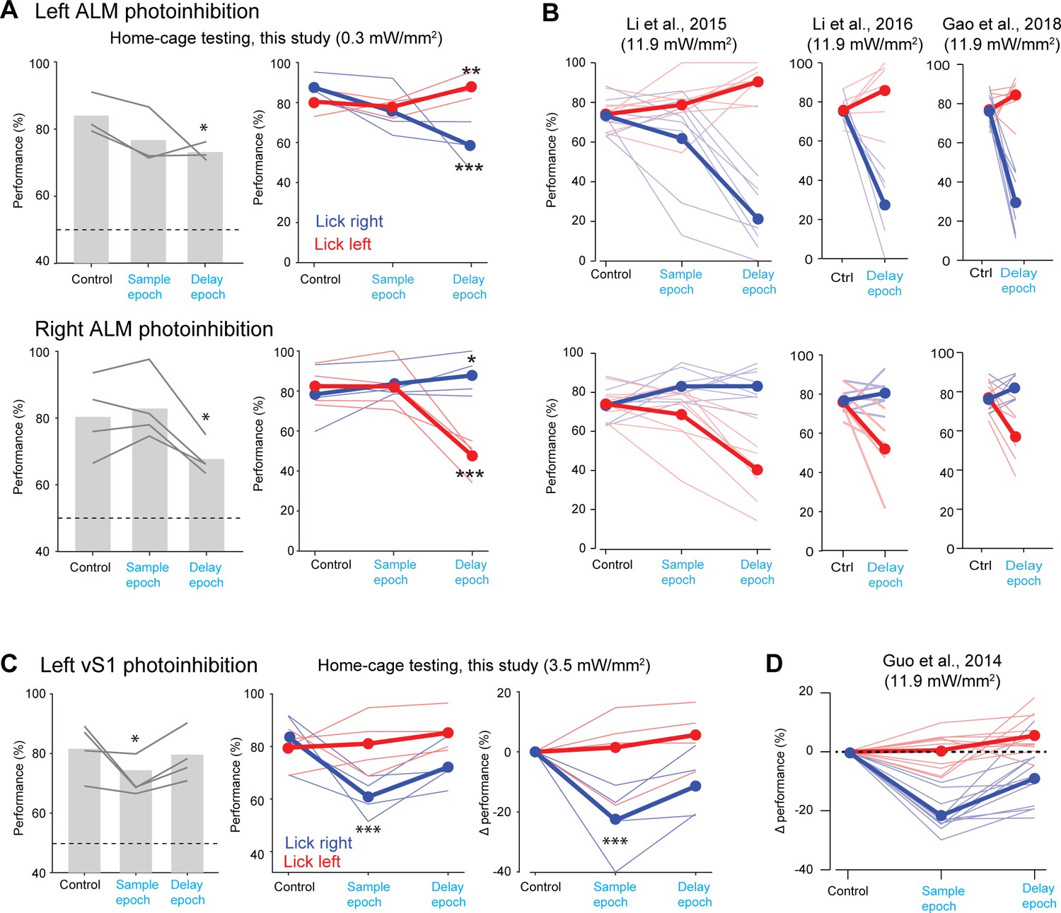
Comparisons of effect size with previous studies.
(A) Behavioral performance during photostimulation of the left ALM (top row) and right ALM (bottom row) in this study. Left, average performance across both trial types. Lines, individual mice. Bar, mean across mice. Dashed line, chance. Right, performance in each trial type. Blue, lick left trials; red, lick right trials. Thin lines, individual mice; thick lines, mean. *p<0.05, **p<0.01, ***p<0.001, significant performance change compared to the control trials (bootstrap, Materials and methods). (B) Behavioral performance during photostimulation of the left ALM (top row) and right ALM (bottom row) from previous studies (Li et al., 2015; Gao et al., 2018; Li et al., 2016). (C) Behavioral performance during photostimulation of the left vS1 in this study. Left, average performance across both trial types. Middle, performance in each trial type. Right, performance change relative to the control trials. (D) Behavioral performance during photostimulation of the left vS1 from previous study (Guo et al., 2014a).
Figure 7—figure supplement 2
Behavioral performance change dose-response curve during optogenetics.
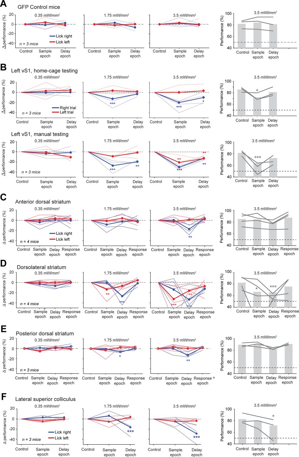
(A) Behavioral performance during photostimulation in the sample or delay epoch. Three mice with only GFP viruses injected into the left ALM. Left, performance change relative to the control trials in each trial type. Blue, lick left trials; red, lick right trials. Thin lines, individual mice; thick lines, mean. Right, average performance across both trial types. Lines, individual mice; bar, mean. Dashed line, chance performance. *p<0.05, **p<0.01, ***p<0.001, significant performance change compared to the control trials (bootstrap, Materials and methods). (B) Same as (A) but for photostimulation of the left vS1 in home-cage optogenetic experiments (top row) and manual optogenetic experiments (bottom row). (C) Same as (A) but for photostimulation of the anterior dorsal striatum. (D) Same as (A) but for photostimulation of the dorsolateral striatum. (E) Same as (A) but for photostimulation of the posterior dorsal striatum. (F) Same as (A) but for photoinhibition of the lateral superior colliculus.
Figure 8 with 1 supplement
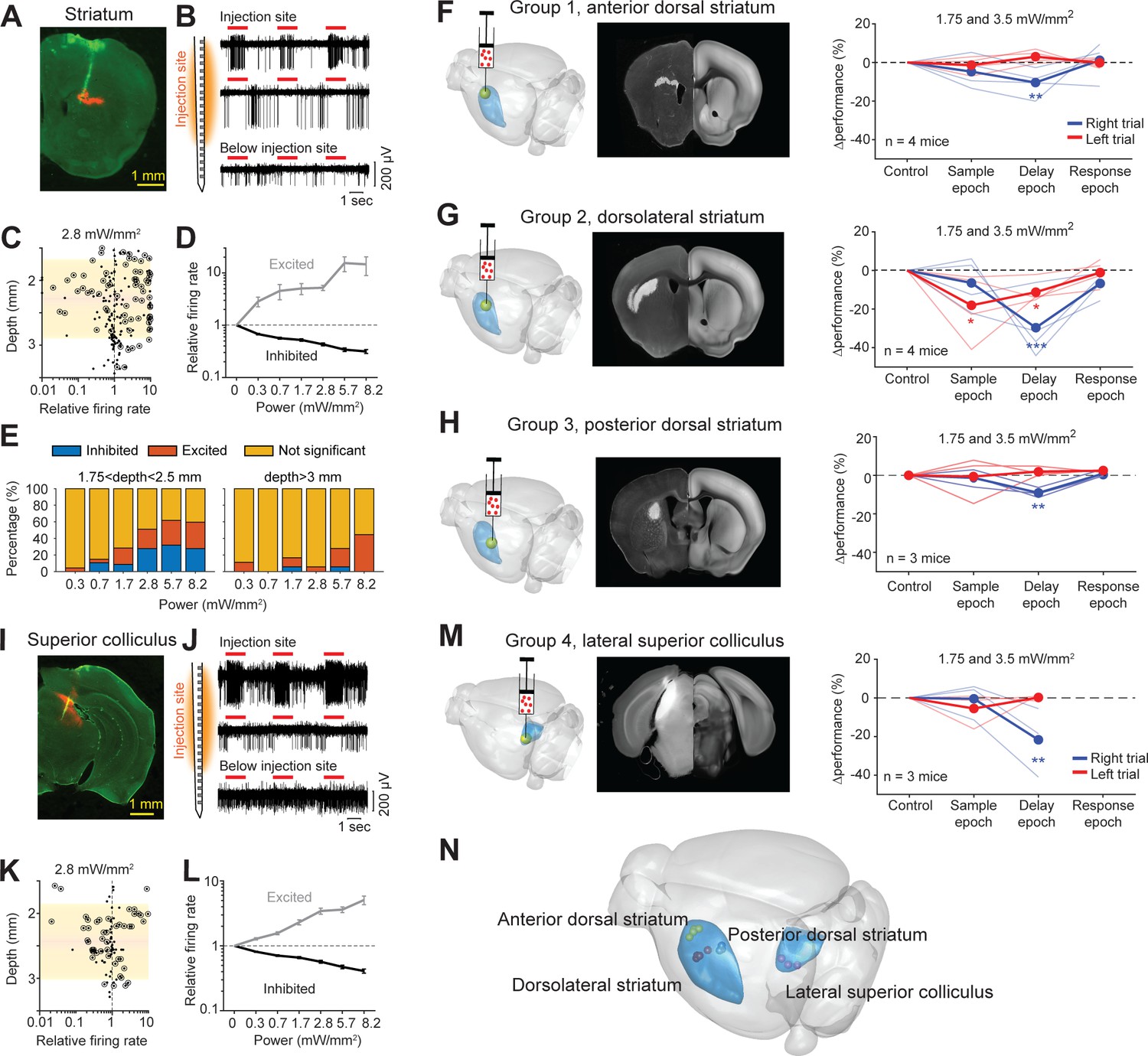
Photostimulation of subcortical regions in home-cage optogenetic experiment.
(A) A coronal section showing virus expression in the striatum (red) and silicon probe recording track (green). (B) Silicon probe recording in the striatum during photostimulation. Multi-unit activity from two example channels near the virus injection site (top) and one example channel below the injection site. Red lines, photostimulation. (C) Effects of photostimulation across depths. Dots correspond to individual neurons. Circled dots indicate neurons with significant spike rate change, p<0.05, two-tailed t-test. Spike rate of each neuron during photostimulation is normalized to its baseline (‘relative firing rate’, Materials and methods). Shaded area indicates the virus expression region estimated from histology. (D) Relative firing rate of all significantly excited and inhibited neurons as a function of photostimulation intensity. Error bars show SEM across neurons. (E) Fraction of neurons significantly excited (red) and inhibited (blue) by photostimulation, p<0.05, two-tailed t-test. Left, neurons from near the virus injection site. Right, neurons from below the virus injection site. (F) Left, a 3D rendered brain showing the striatum (blue) and the injection location in the anterior dorsal striatum (yellow). Middle, a coronal section showing example virus expression. The coronal section is aligned to the Allen Reference Brain (Materials and methods). Right, behavioral performance change relative to the control trials during photostimulation in the sample, delay, or response epoch. Blue, lick left trials; red, lick right trials. Thin lines, individual mice; thick lines, mean. **p<0.01, ***p<0.001, significant performance change compared to the control trials (bootstrap, Materials and methods). (G) Same as (F) but for photostimulation in the dorsolateral striatum. (H) Same as (F) but for photostimulation in the posterior dorsal striatum. (I–L) Same as (A–D) but for photoinhibition in the left superior colliculus. (M) Same as (E) but for photoinhibition in the left superior colliculus. (N) The 3D rendered brain shows the striatum and superior colliculus (blue) and the centers of virus expression in individual mice used in this study (dots). See individual mouse data in Figure 8—figure supplement 1.
Figure 8—figure supplement 1
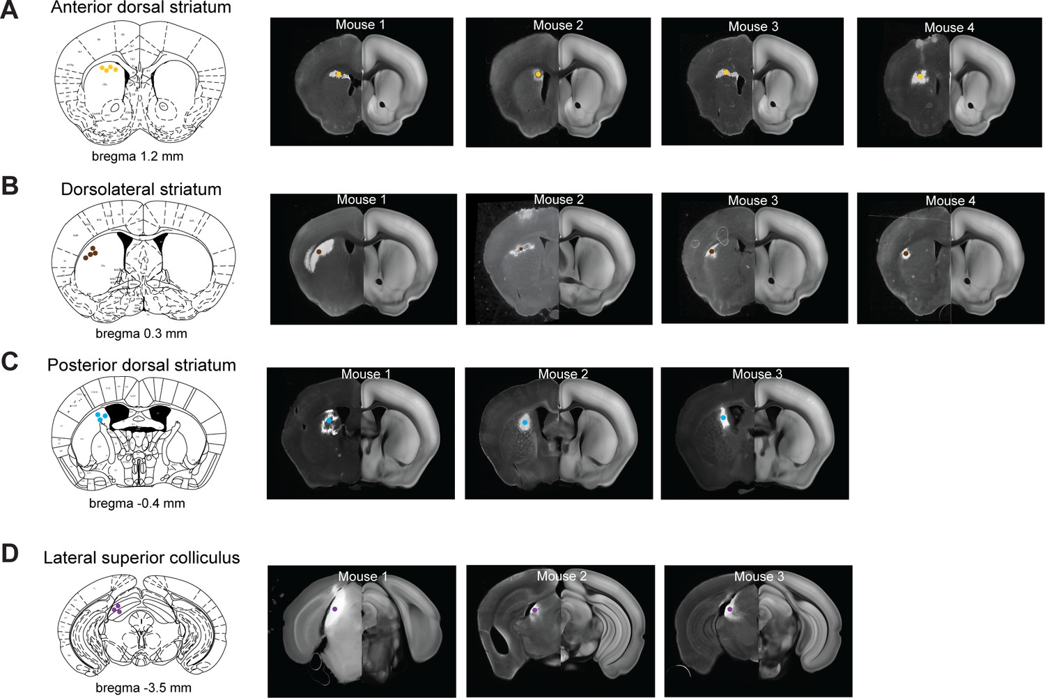
Virus injection sites in the striatum and superior colliculus.
(A) Left, a coronal section showing the centers of virus expression in individual mice (yellow dots). Right, coronal sections of individual mice showing virus expression in the anterior dorsal striatum. The coronal sections are aligned to the Allen Reference Brain (Materials and methods). (B) Same as (A) but for the dorsolateral striatum. (C) Same as (A) but for the posterior dorsal striatum. (D) Same as (A) but for the lateral superior colliculus.
Videos
Video 1
A mouse performing voluntary head-fixation, tactile decision task, and self-release in home-cage.
A mouse voluntarily pokes into the headport and gets head-fixed. Once head-fixed, a trial is initiated. A pole drops into the whisker field at specific locations for 1.3 s then retracts (‘sample’). After another 1.3 s (‘delay’), an auditory go cue is played, and the mouse licks the left or right lickspouts to report choice (‘response’). The mouse is released after 60 s of head-fixation (‘time-up release’). The mouse also self-releases by pressing against the floor (‘self-release’).
Video 2
Optogenetic photostimulation during task performance in home-cage.
In a subset of trials, 630 nm light is turned on during either the sample or delay epoch. Photostimulation is through a clear skull implant to activate red-shifted opsins expressed in specific brain regions. During unsupervised optogenetic testing, the light source is positioned over the targeted brain region. In addition, a 630 nm masking flashing is given in every trial to prevent the mouse from distinguishing the trials with photostimulation. The masking flash is turned off in this example video for demonstration purposes.
Tables
Key resources table
| Reagent type (species) or resource | Designation | Source or reference | Identifiers | Additional information |
|---|---|---|---|---|
| Strain, strain background (Mouse) | Gad2-IRES-Cre | The Jackson Laboratory | JAX: 010802 (RRID:IMSR_JAX:014548) | Cre targeted at theGad2 locus |
| Strain, strain background (Mouse) | PV-IRES-Cre | The Jackson Laboratory | JAX: 008069 (RRID:IMSR_JAX:008069) | Cre targeted at thePvalb locus |
| Strain, strain background (Mouse) | VGAT-ChR2-EYFP | The Jackson Laboratory | JAX: 014548 (RRID:IMSR_JAX:014548) | ChR2 targeted at theSlc32a1 locus |
| Strain, strain background (Mouse) | Ai32(RC-hR2(H134R)/EYFP) | The Jackson Laboratory | JAX: 012569 (RRID:IMSR_JAX:012569) | ChR2 targeted at theGt(ROSA)26Sor locus |
| Recombinant DNA reagent | AAV9-hSyn-FLEX-ChrimsonR-tdTomato | UNC Viral Core | N/A | |
| Recombinant DNA reagent | AAV8-Ef1a-DIO-ChRmine-mScarlet-WPRE | Stanford Viral Core | GVVC-AAV-188 | |
| Recombinant DNA reagent | AAV-pCAG-FLEX-EGFP-WPRE | Addgene | 51502 (RRID:Addgene_51502) | |
| Software, algorithm | MATLAB | Mathworks | https://www.mathworks.com | |
| Other | Design files, software, and documentations for the automated home-cage system. | This paper - Github repository | https://github.com/NuoLiLabBCM/Autocage | The Github repository contains the hardware design files and software for the construction of automated home-cage system, along with documentations and protocols for automated head-fixation training and task training. |
Additional files
-
Supplementary file 1
Comparison with previous automated home-cage training systems with voluntary head-fixation.
- https://cdn.elifesciences.org/articles/66112/elife-66112-supp1-v2.docx
-
Transparent reporting form
- https://cdn.elifesciences.org/articles/66112/elife-66112-transrepform-v2.docx
Download links
A two-part list of links to download the article, or parts of the article, in various formats.
Downloads (link to download the article as PDF)
Open citations (links to open the citations from this article in various online reference manager services)
Cite this article (links to download the citations from this article in formats compatible with various reference manager tools)
Fully autonomous mouse behavioral and optogenetic experiments in home-cage
eLife 10:e66112.
https://doi.org/10.7554/eLife.66112


