Stability of neocortical synapses across sleep and wake states during the critical period in rats
- Department of Biology, Brandeis University, United States
Figures
Figure 1 with 2 supplements
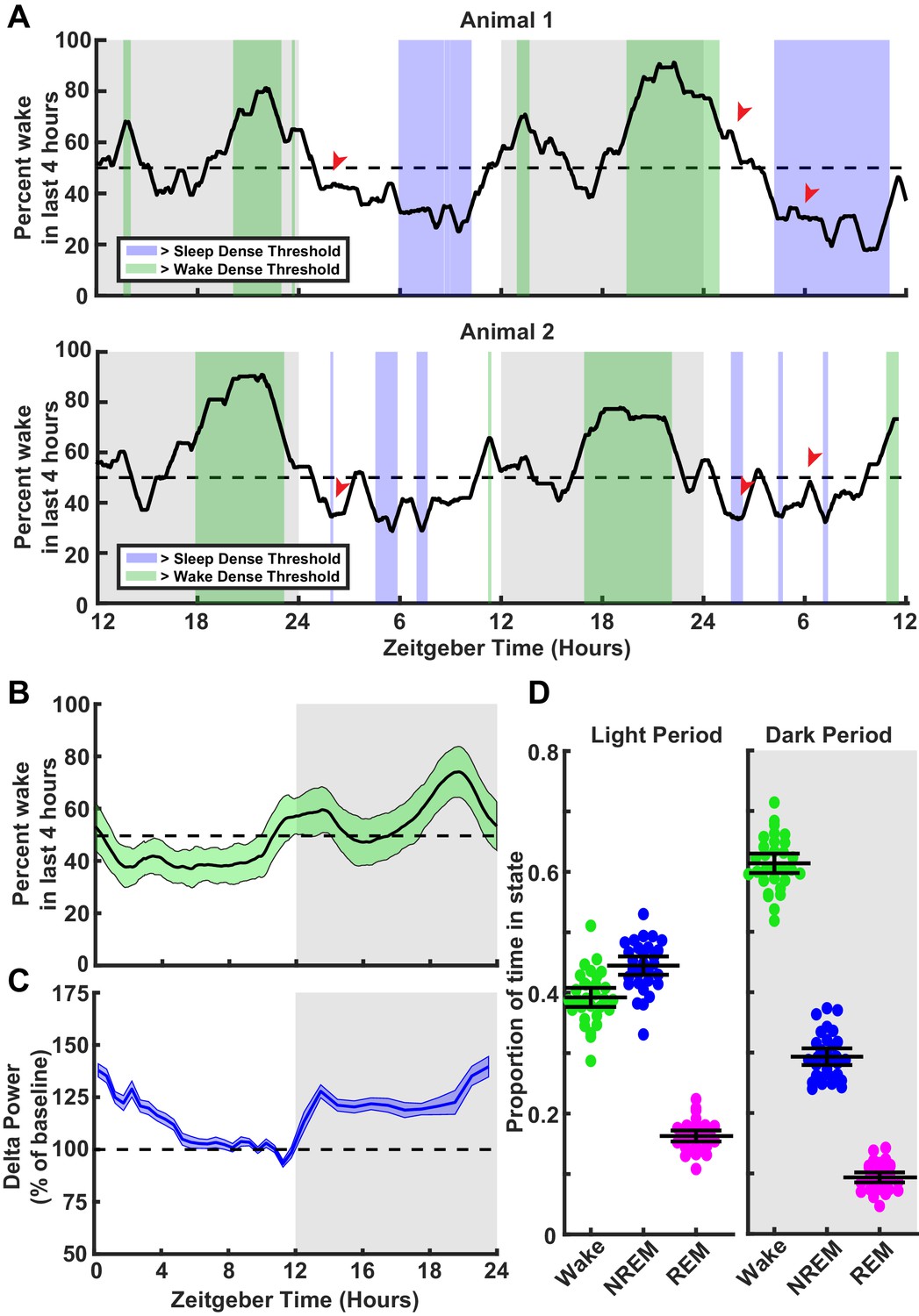
Characterization of sleep/wake behavior in juvenile Long-Evans rats.
(A) Two example sleep/wake histories from two different animals. The y axis is a moving mean showing percent of time spent awake in the previous 4 hr; x axis is zeitgeber time (ZT) in hours. Periods where the animal is in a sleep-dense epoch (>65% time asleep in previous 4 hr) are colored blue, while >65% wake in previous 4 hr are colored green. Red arrows indicate points showing differing sleep/wake-dense experiences between animals at the same ZT. (B) Average percentage time spent awake in the previous 4 hr as a function of ZT. Light green shading indicates the standard deviation between animals; n = 30 animals. (C) Normalized delta power from the electroencephalogram (EEG) of animals in (B) as a percent of baseline (hours 7–11 in the light period). Shading represents SEM between animals. (D) Average time spent in each behavioral state shown as a proportion for each animal broken down by light period (left) and dark period (right); each point represents one animal. Mean and SEM shown, n = 30 animals.
Figure 1—figure supplement 1
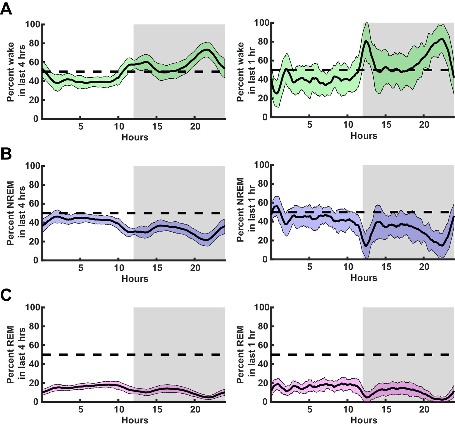
Behavioral state breakdown over circadian cycle in juvenile Long-Evans rats.
(A) Left, average percentage time spent awake in the previous 4 hr as a function of zeitgeber time (ZT). Right, same as left but in last 1 hr. (B) Same as in (A) but shows percentage of time spent in non-rapid eye movement (NREM) sleep. (C) Same as in (A,B) but shows percentage of time spent in rapid eye movement (REM) sleep. Mean and standard deviation shown, n = 30 animals.
Figure 1—figure supplement 2
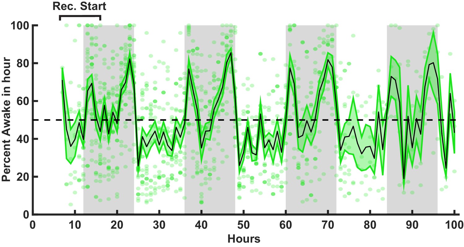
Stable sleep history in animals used in ex vivo slice experiments.
Percent time spent awake for animals used in ex vivo slice recordings in 1 hr bins. Recordings for each animal started within the indicated window. Black line = mean, green shading = SEM, each dot = data from one animal for 1 hr. Gray bars indicate dark period. n = 25 animals.
Figure 2 with 1 supplement

Real-time behavioral classification.
(A) One hour of behavioral data illustrating variables used for classification of sleep/wake state, described in descending order. Top shows expanded raw electroencephalogram (EEG) traces from the indicated periods; scale bar next to non-rapid eye movement (NREM) example, 1 V, 0.5 s. Below expanded EEG is the sleep/wake classification expressed as a hypnogram, where colored bars indicate periods of wake (green), NREM (blue), or rapid eye movement (REM) (magenta). Beneath the hypnogram is the full raw EEG trace; scale is 2 V. Spectral frequency (Spect. Freq.) plots the full spectrogram of the EEG from 0 to 20 Hz, colored by power (normalized to maximum). Extracted features of the Spect. Freq. are plotted below: delta(0.5–4 Hz)/beta(20–35 Hz) power ratio (shown on log scale) is high during periods of NREM, while the theta(5–8 Hz)/delta(0.5–4 Hz) power ratio is high during periods of REM. Absolute electromyogram (EMG) values were normalized and expressed as standard deviation. Finally, animal movement in pixels is plotted. The bottom four plots of vigilance state features each have an adjustable threshold for state classification, shown as dashed line; points above the threshold are shown as colored dots. (B) Schematic of real-time classifier rig. (C) 3D plot of vigilance state features: delta ratio, theta ratio, and movement measures (zero movement assigned lowest observed value for log axis) colored by brain state. Data from example animal. (D) Accuracy of real-time classifier compared to manual scoring by state: overall (% time matching between all three states)=93.3%; wake = 94.2%; NREM = 93.2%; REM = 90.5%; wake dense (matching wake dense on and off times)=96.0%; sleep dense = 96.0%.
Figure 2—figure supplement 1
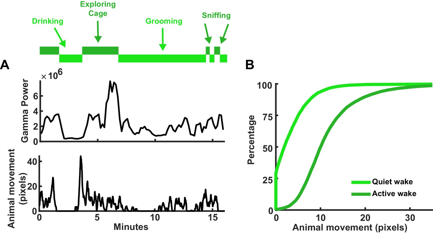
Discrimination of active and quiet wake.
(A) Top, hypnogram indicating periods of active (dark green) or quiet (light green) wake. Some states labeled with specific activities the animal was performing, as determined by video recording. Top line plot is the gamma power of the local field potential (LFP), which is higher during more active wake behaviors. Bottom line plot is the animal’s movement in pixels; higher movement is associated with active wake. (B) Cumulative plot of the animal’s movement (same animal from A) for active and quiet wake states.
Figure 3 with 2 supplements
Stability of miniature excitatory postsynaptic current (mEPSC) amplitude after prolonged periods of sleep or wake.
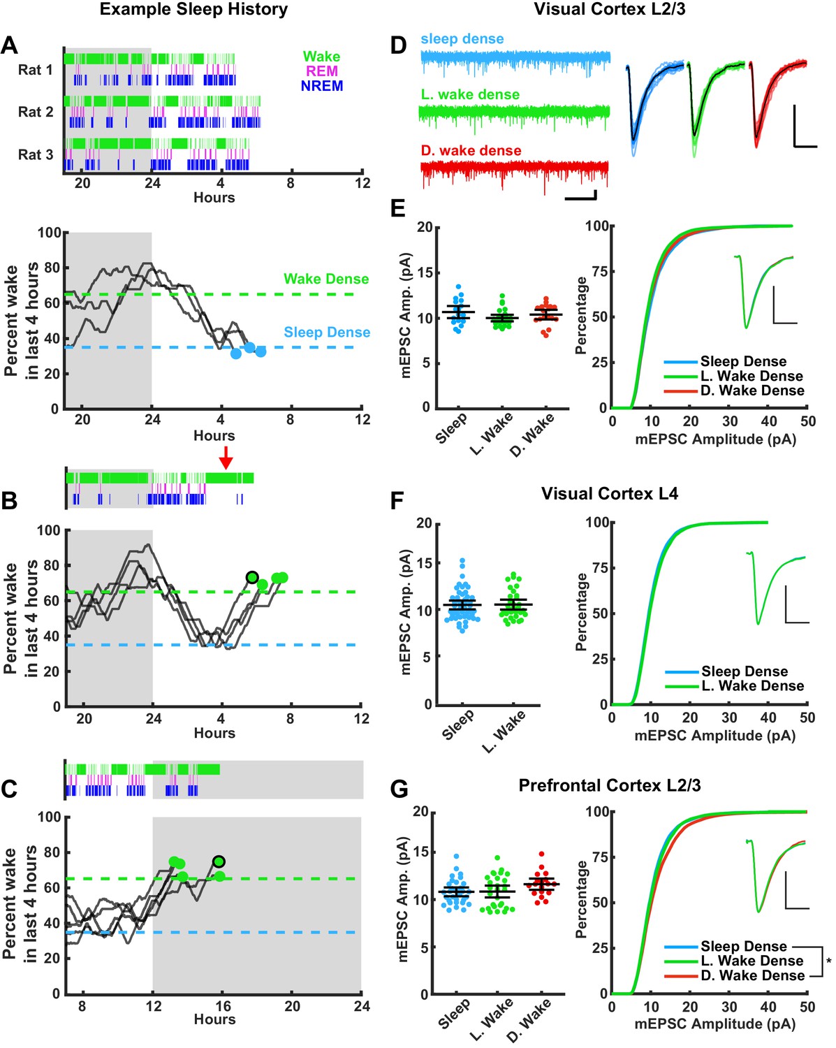
The left column represents example sleep histories for the VC L2/3 experiments while right column shows mEPSC characteristics for the indicated cell types and brain regions. (A) Top figure, hypnograms for three animals used for sleep-dense mEPSC recordings. Green bars indicate instances of wake, magenta indicates rapid eye movement (REM), and blue non-rapid eye movement (NREM). Bottom, this same behavioral state data represented as a moving average of % time spent awake in the preceding 4 hr; the dashed lines represent the thresholds for achieving the required density in a given state, and the dots represent endpoints for slice recordings. (B) and (C) are same as for (A), but for wake-dense recordings performed during the light and dark periods, respectively. Red arrow indicates wake encouragement (introduction of toy). Black circle around endpoint dot indicates which trace is represented by example hypnogram. (D) Traces on the left, example mEPSC recordings from L2/3 of primary visual cortex (V1); scale bar, 10 pA, 1 s. On the right, cell average mEPSC events; scale bar, 5 pA, 5 ms. (E) On left, cell average mEPSC amplitudes from L2/3 V1; error bars = 95% CI of mean (p=0.17; Kruskal-Wallis). (E) On right, cumulative histogram of sampled mEPSC amplitudes (SD – L. WD p=0.075, L. WD – D. WD p>0.9, SD – D. WD p=0.77; Kolmogorov-Smirnov (KS) test with Bonferroni correction). Inset for (E)–(G) is a peak scaled average mEPSC waveform; scale bar, 50% peak, 5 ms. Sleep dense n = 17 cells, three animals; L. wake dense n = 25 cells, four animals; D. wake dense n = 18 cells, five animals. (F) On left, cell average mEPSC from L4 V1 (p=0.52; Kruskal-Wallis). (F) On right, cumulative mEPSC amp. from L4 V1 (p=0.99; KS test). Sleep dense n = 47 cells, six animals; L. wake dense n = 32 cells, four animals. (G) On left, cell average mEPSC amplitudes from L2/3 prefrontal cortex (PFC) (p=0.13; Kruskal-Wallis). (G) On right, cumulative histogram of sampled mEPSC amplitudes (SD – L. WD p>0.9, L. WD – D. WD p=0.096, SD – D. WD p=0.015; KS test with Bonferroni correction). Sleep dense n = 31 cells, six animals; L. wake dense n = 28 cells, five animals; D. wake dense n = 18 cells, six animals.
Figure 3—figure supplement 1
Sleep/wake histories for additional ex vivo slice recordings.
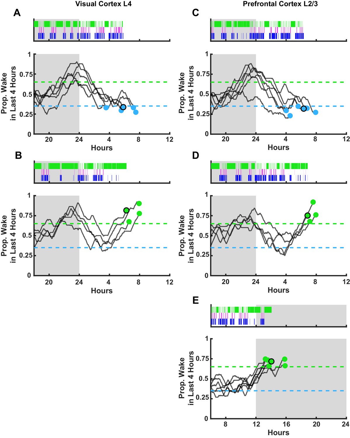
Each experiment includes an example hypnogram from one animal above summary data of wake history. (A) Animals from visual cortex L4 recordings. Top figure, example hypnogram from a single animal. Green bars indicate instances of wake, magenta indicates rapid eye movement (REM), and blue non-rapid eye movement (NREM). Below, this same behavioral state data is represented as a moving average of % time spent awake in the preceding 4 hr but for each animal included in the experiment; the dashed lines represent the thresholds for achieving the required density in a given state, and the dots represent endpoints for slice recordings. Black circle around endpoint dot indicates which trace is represented by example hypnogram. (B) Same as (A) but for wake-dense recordings (with green dots). (C–D) Same as (A–B) but for prefrontal cortex L2/3 recordings. (E) Same as (D) but for the D. wake-dense recordings (i.e. sacrifice occurred in the dark period).
Figure 3—figure supplement 2

Drop in delta power and time spent awake do not correlate with miniature excitatory postsynaptic current (mEPSC) amplitudes or frequency.
(A) Schematic showing how drop in delta power is calculated. Delta drop was calculated as percentage drop from sleep epochs that occurred in the window zeitgeber time (ZT) 23.5–1.5 to the last hour of sleep right before sacrificing animals. Peak delta power after extended wake at t1 is normalized to the baseline recovery period of t2. (B) mEPSC amplitude after a sleep-dense epoch, plotted against normalized drop in delta power during that epoch. Black line = linear fit; R2 value and p-value included on plot. Cell averages from different regions are indicated in legend. (C) Same as (B) but for mEPSC frequency. (D) Schematic illustrating time spent awake in preceding 4 hr of a wake-dense epoch. (E) mEPSC amplitude after a wake-dense epoch, plotted against proportion of time spent awake in previous 4 hr. Cell averages from different regions are indicated in legend; light period recordings in green, dark period recordings in red. (F) Same as (E) but for mEPSC frequency.
Figure 4
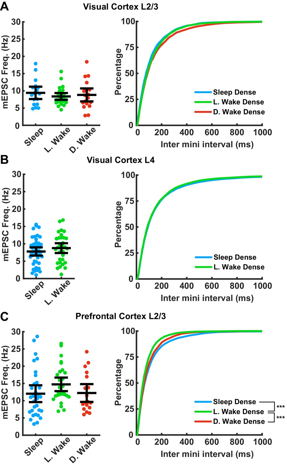
Impact of prolonged sleep/wake on miniature excitatory postsynaptic currents (mEPSC) frequency.
mEPSC frequency is not consistently modulated by sleep/wake history across brain regions. (A) Data from visual cortex L2/3. Left plot, cell average mEPSC frequencies for the indicated conditions; error bars = 95% CI of mean (p=0.75, Kruskal-Wallis). Right plot, cumulative plot of inter-event interval (SD − L. WD p=0.35, SD − D. WD p=0.15, L. WD − D. WD p>0.9; Kolmogorov-Smirnov (KS) test with Bonferroni correction). Sleep dense n = 17 cells, three animals; L. wake dense n = 25 cells, four animals; D. wake dense n = 18 cells, five animals. (B) Same as in (A) but data from visual cortex L4; cell average on left (p>0.9, Kruskal-Wallis); cumulative plot on right (p=0.45, KS test). Sleep dense n = 47 cells, six animals; L. wake dense n = 32 cells, four animals. (C) Same as in (A) but data from prefrontal cortex L2/3. Left, cell average values for the indicated conditions (p=0.056, Kruskal-Wallis). Cumulative plot of inter-event interval (SD − L. WD p<1e-6, SD − D. WD p=0.74, L. WD − D. WD p=0.007; KS test with Bonferroni correction). Sleep dense n = 31 cells, six animals; L. wake dense n = 28 cells, five animals; D. wake dense n = 18 cells, six animals.
Figure 5
Thalamocortical (TC) evoked synaptic responses in freely behaving animals.
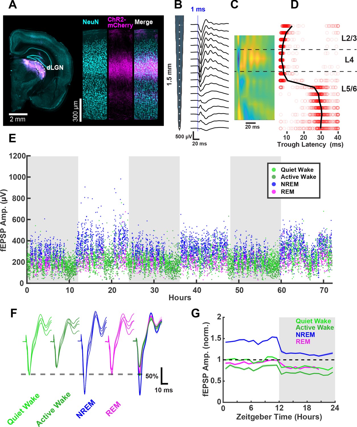
(A) AAV-Chr2-mCherry viral expression targeted to dorsal lateral geniculate nucleus (dLGN) projects to V1. Left, coronal slice showing viral expression in magenta. Right, visual cortex showing neuronal nuclei marked with NeuN and ChR2-mCherry in magenta. (B) Evoked field excitatory postsynaptic potentials (fEPSPs) recorded with a linear silicon array show clear layer-specific waveforms consistently with TC afferent location. (C) Current source density heat plot identifies layers; cool colors indicate current sink. (D) fEPSP latency to first negative peak identifies layers. Red circles represent latency of individual events; black line represents mean for each channel. (E) fEPSPs recorded over 3 days in a single freely behaving animal. Amplitude of the response plotted and colored by brain state. Dark periods (lights off) are represented by gray rectangles. (F) fEPSP waveforms by brain state, where each waveform is from a different animal; normalized to QW peak (indicated by dashed line) for each animal. Scale bar, 50% of peak amplitude, 10 ms. (G) fEPSP amplitudes across circadian time, normalized to quiet wake in the light period. n = 4 animals.
Figure 6 with 1 supplement
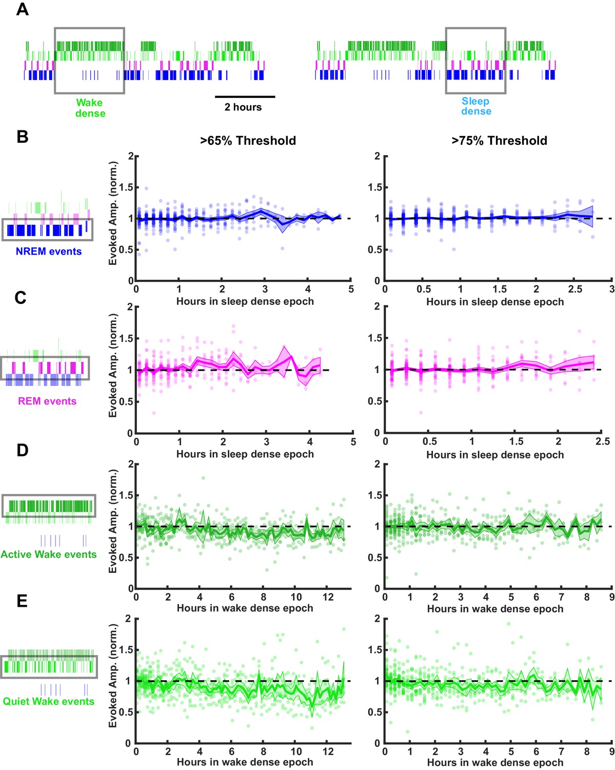
Stability of thalamocortical field excitatory postsynaptic potential (fEPSP) amplitude during prolonged periods of sleep or wake.
Time series data of thalamocortical evoked fEPSPs over the course of either sleep- or wake-dense epochs. (A) Example hypnograms showing wake- (left) and sleep- (right) dense epochs. Gray rectangles indicate times in which stimulations were analyzed for this example. (B) fEPSP amplitudes during sleep-dense epochs, measured in non-rapid eye movement (NREM) (as illustrated by box around hypnogram on left). Epochs passing the >65% threshold are shown on left, and those passing the >75% threshold are shown on right. fEPSP amplitude was normalized to the beginning of each epoch. Each dot is data from one epoch, averaged over 10 min bins; n = 4 animals. Blue line = mean, shading = SEM, black dotted line = 1 (i.e. no change). (C) Same as (B) but for rapid eye movement (REM) events. (D) Same as (B) but normalized fEPSP amplitude during wake, measured during active wake. (E) Same as (D) but for quiet wake events.
Figure 6—figure supplement 1
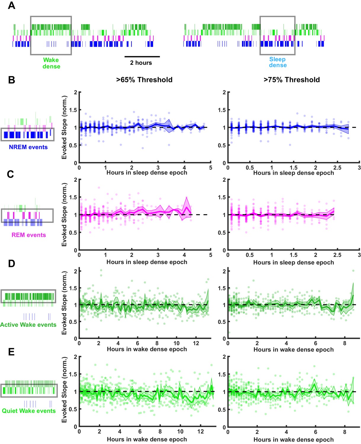
Stability of field excitatory postsynaptic potential (fEPSP) slope during prolonged periods of sleep or wake.
Time series data of thalamocortical evoked fEPSP slopes over the course of either sleep- or wake-dense epochs. (A) Hypnograms showing an example of a wake- and sleep-dense epoch. Black rectangles indicate example times in which stimulations were analyzed for this example. (B) fEPSP slopes during sleep-dense epochs, measured in non-rapid eye movement (NREM) (as illustrated by box around hypnogram on left). Epochs passing the >65% threshold are shown on left, and those passing the >75% threshold are shown on right. fEPSP slope was normalized to the beginning of each epoch. Each dot is data from one epoch, averaged over 10 min bins; n = 4 animals. Blue line = mean, shading = SEM, black dotted line = 1 (i.e. no change). (C) Same as (B) but for rapid eye movement (REM) events. (D) Same as (B) but normalized fEPSP slope during wake, measured during active wake. (E) Same as (D) but for quiet wake events.
Figure 7

Thalamocortical field excitatory postsynaptic potential (fEPSP) amplitude measured before and after prolonged periods of sleep or wake.
(A) Hypnograms showing an example of a wake- (left) and sleep- (right) dense epoch, with flanking periods of the opposite state. Gray rectangles indicate when measurements were taken for comparison. (B) Example fEPSP waveforms before and after a wake- (left) or sleep- (right) dense epoch. (C) Normalized change in fEPSP amplitude after wake or sleep (wake change, p>0.9; sleep change, p>0.9; Wilcoxon signed-rank test). (D) Correlative plot of duration of wake-dense epoch against normalized change in fEPSP amplitude. Black line = linear fit; R2 value and p-value included on plot. Inset in top right is an expansion of plot between 0 and 3.5 hr. (E) Same as (D) but for sleep dense. n = 39 wake-dense epochs, 55 sleep-dense epochs, four animals.
Figure 8
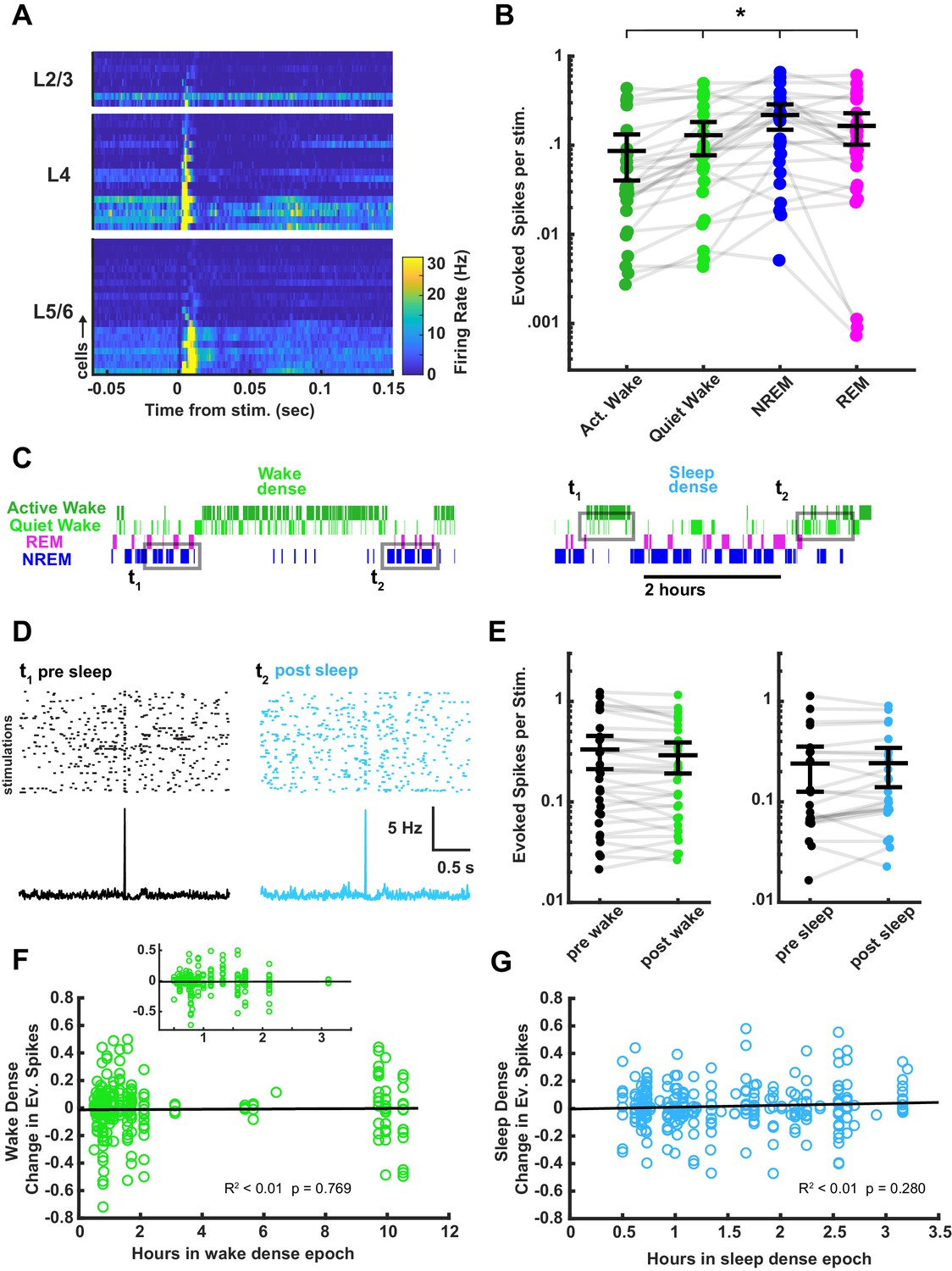
Characterization of thalamocortical evoked spiking in visual cortex between behavioral states and its stability across sleep and wake.
(A) Heat plot response of the firing rate of each cell isolated during stimulation. Data are grouped by layer and sorted by the magnitude of response within each layer. n = 45 cells, four animals. (B) Evoked spikes per stimulation for each of the four vigilance states. The y axis represents the average number of evoked spikes for a single stimulation, calculated as spikes in a 15 ms post-stimulus window, minus the expected number of baseline spikes in that window; each dot represents a cell. Evoked spikes varied significantly by vigilance state (AW-QW, p=3.4e-4; AW-NREM, p=6.56e-4; AW-REM, p=4.70e-4; QW-NREM, p=0.0022; QW-REM, p=0.0122; NREM-REM, p=0.0380). (C) To determine whether evoked spike rates were affected by time spent awake or asleep, we compared evoked spiking before and after a sleep- or wake-dense epoch, using a >75% time in state threshold, as for field excitatory postsynaptic potentials (fEPSPs) in Figure 7. Hypnograms show examples of wake- or sleep-dense epochs with flanking periods of the opposite state. Gray rectangles indicate the stimulation times chosen for the analysis. (D) Example raster plots and post-stimulus time histograms of firing rate for an example cell pre-post sleep. (E) The number of evoked spikes before and after wake- (left) or sleep- (right) dense epochs; each dot is one cell, averaged across all of the wake- or sleep-dense epochs (wake dense n = 32 cells, four animals; sleep dense n = 24 cells, four animals). (F) Correlative plot of duration of wake-dense epoch against change in evoked spikes; each dot represents the response of a single cell to a single epoch (post – pre). Black line = linear fit; R2 value and p-value included on plot. Inset is an expansion of plot between 0.25 and 3.5 hr. (G) Same as (F) but for sleep-dense epochs. n = 35 wake-dense epochs, 50 sleep-dense epochs, four animals.
Author response image 1
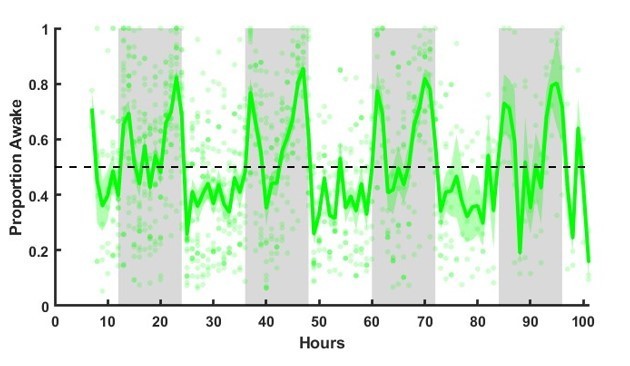
Sleep history from start of EEG recording for animals used for slice experiments.
Unperturbed sleep patterns from initiation of EEG recordings, which started 2-3 days postsurgery. Dots show proportion of time spent awake for individual animals (averaged in 1 hr bins). Green line shows average across animals, shading = SEM. Sleep/wake behavior stabilized soon (roughly 4-8 hr) after the initiation of recording..
Author response image 2
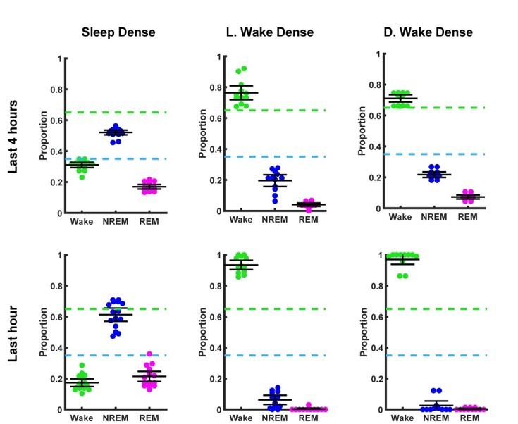
Endpoint behavioral state proportions.
Top row (Last 4 hrs), represents the relative time spent in each behavioral state in the last 4 hrs prior to sacrifice for each individual animal used for ex vivo slice recording. The top row is separated in to three columns for each type of experiment. From left to right, sleep dense experiments (in light period), light period wake dense experiments, dark period wake dense experiments. Green and blue dotted lines represent wake (>65%) and sleep (<35%) dense thresholds, respectively. Bottom row (Last hour), is identical to the top row but for the last hours of time prior to sacrifice. Black bars represent mean and 95% confidence interval.
Author response image 3
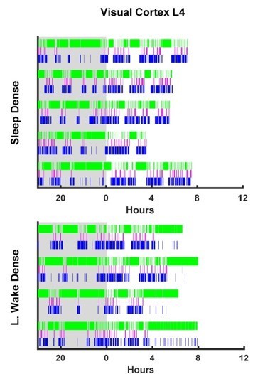
Visual Cortex L4 hypnograms.
Here the hypnograms for each individual animal used in L4 visual cortex ex vivo slice experiments are plotted. Green bars indicate instances of wake, magenta indicates REM, and blue NREM. Grey rectangle indicates hours when lights are off (i.e. the dark period). Top plot, hypnograms for animals in the light period sleep dense experiment. Bottom plot, hypnograms from light period wake dense experiment.
Author response image 4
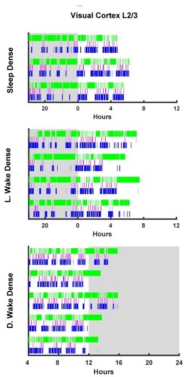
Visual Cortex L2/3 hypnograms.
Here the hypnograms for each individual animal used in L2/3 visual cortex ex vivo slice experiments are plotted. Green bars indicate instances of wake, magenta indicates REM, and blue NREM. Grey rectangle indicates hours when lights are off (i.e. the dark period). Top plot, hypnograms for animals in the light period sleep dense experiment. Middle plot, hypnograms from light period wake dense experiment. Bottom plot, hypnograms from dark period wake dense experiment.
Author response image 5
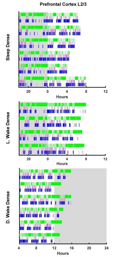
Prefrontal Cortex L2/3 hypnograms.
Here the hypnograms for each individual animal used in L2/3 prefrontal cortex ex vivo slice experiments are plotted. Green bars indicate instances of wake, magenta indicates REM, and blue NREM. Grey rectangle indicates hours when lights are off (i.e. the dark period). Top plot, hypnograms for animals in the light period sleep dense experiment. Middle plot, hypnograms from light period wake dense experiment. Bottom plot, hypnograms from dark period wake dense experiment.
Tables
Key resources table
| Reagent type (species) or resource | Designation | Source or reference | Identifiers | Additional information |
|---|---|---|---|---|
| Strain, strainbackground (Rattus norvegicus) | Long-Evans Rat | Charles River Labs | Charles River 006; RRID:RGD_2308852 | |
| Recombinant DNA reagent | AAV-ChR2(H134R)-mCherry | UPenn Vector Core | Penn ID: AV-9–20938M; Addgene: 100054-AAV9 |
Additional files
Download links
A two-part list of links to download the article, or parts of the article, in various formats.
Downloads (link to download the article as PDF)
Open citations (links to open the citations from this article in various online reference manager services)
Cite this article (links to download the citations from this article in formats compatible with various reference manager tools)
Stability of neocortical synapses across sleep and wake states during the critical period in rats
eLife 10:e66304.
https://doi.org/10.7554/eLife.66304


