Temporally delayed linear modelling (TDLM) measures replay in both animals and humans
- State Key Laboratory of Cognitive Neuroscience and Learning, IDG/McGovern Institute for Brain Research, Beijing Normal University, China
- Chinese Institute for Brain Research, China
- Max Planck University College London Centre for Computational Psychiatry and Ageing Research, United Kingdom
- Wellcome Centre for Human Neuroimaging, University College London, United Kingdom
- Wellcome Centre for Integrative Neuroimaging, University of Oxford, United Kingdom
- Center for Brains, Minds and Machines, Picower Institute for Learning and Memory, Department of Brain and Cognitive Sciences, Massachusetts Institute of Technology, United States
- Donders Institute for Brain Cognition and Behaviour, Radboud University, Netherlands
- Research Department of Cell and Developmental Biology, University College London, United Kingdom
- DeepMind, United Kingdom
Figures
Figure 1 with 1 supplement
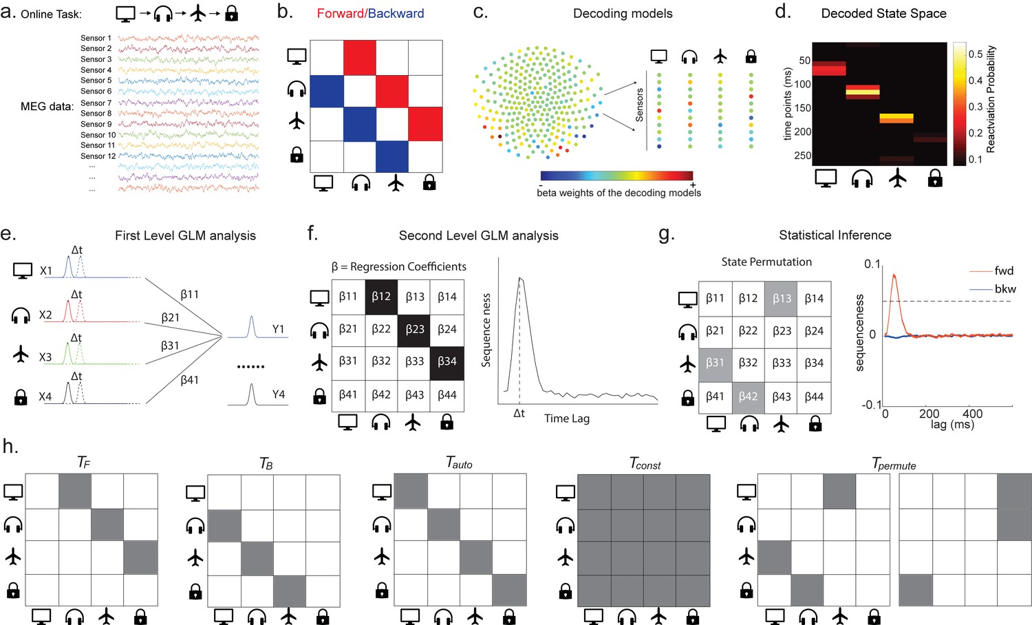
Task design and illustration of temporal delayed linear modelling (TDLM).
(a) Task design in both simulation and real MEG data. Assuming there is one sequence, A->B->C->D, indicated by the four objects at the top. During the task, participants are shown the objects and asked to figure out a correct sequence for these objects while undergoing MEG scanning. A snapshot of MEG data is shown below. It is a matrix with dimensions of sensors by time. (b) The transitions of interest are shown, with the red and blue entries indicating transitions in the forward and backward direction, respectively. (c) The first step of TDLM is to construct decoding models of states from task data, and (d) then transform the data (e.g. resting-state) from sensor space to the state space. TDLM works on the decoded state space throughout. (e) The second step of TDLM is to quantify the temporal structure of the decoded states using multiple linear regressions. The first-level general linear modelling (GLM) results in a state*state regression coefficient matrix (empirical transition matrix), , at each time lag. (f) In the second-level GLM, this coefficient matrix is projected onto the hypothesized transition matrix (black entries) to give a single measure of sequenceness. Repeating this process for the number of time lags of interest generates sequenceness over time lags (right panel). (g) The statistical significance of sequenceness is tested using a non-parametric state permutation test by randomly shuffling the transition matrix of interest (in grey). To control for multiple comparisons, the permutation threshold is defined as the 95th percentile of all shuffles on the maximum value over all tested time lags. (h) The second-level regressors , , , and , as well as two examples of the permuted transitions of interest, (for constructing permutation test), are shown.
Figure 1—figure supplement 1
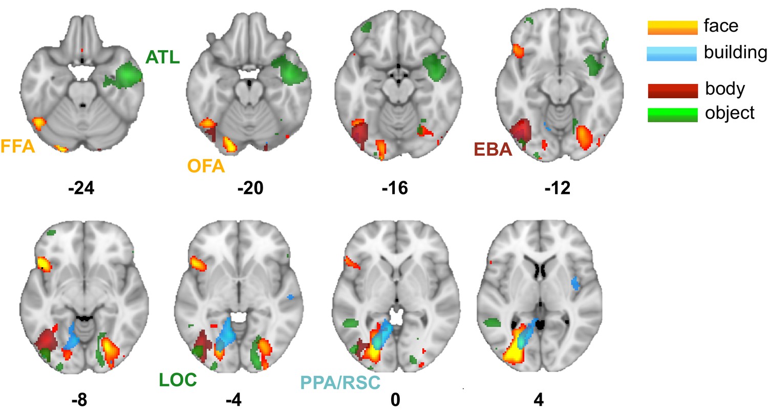
Source localization of stimuli-evoked neural activity in MEG.
Figure 2 with 1 supplement
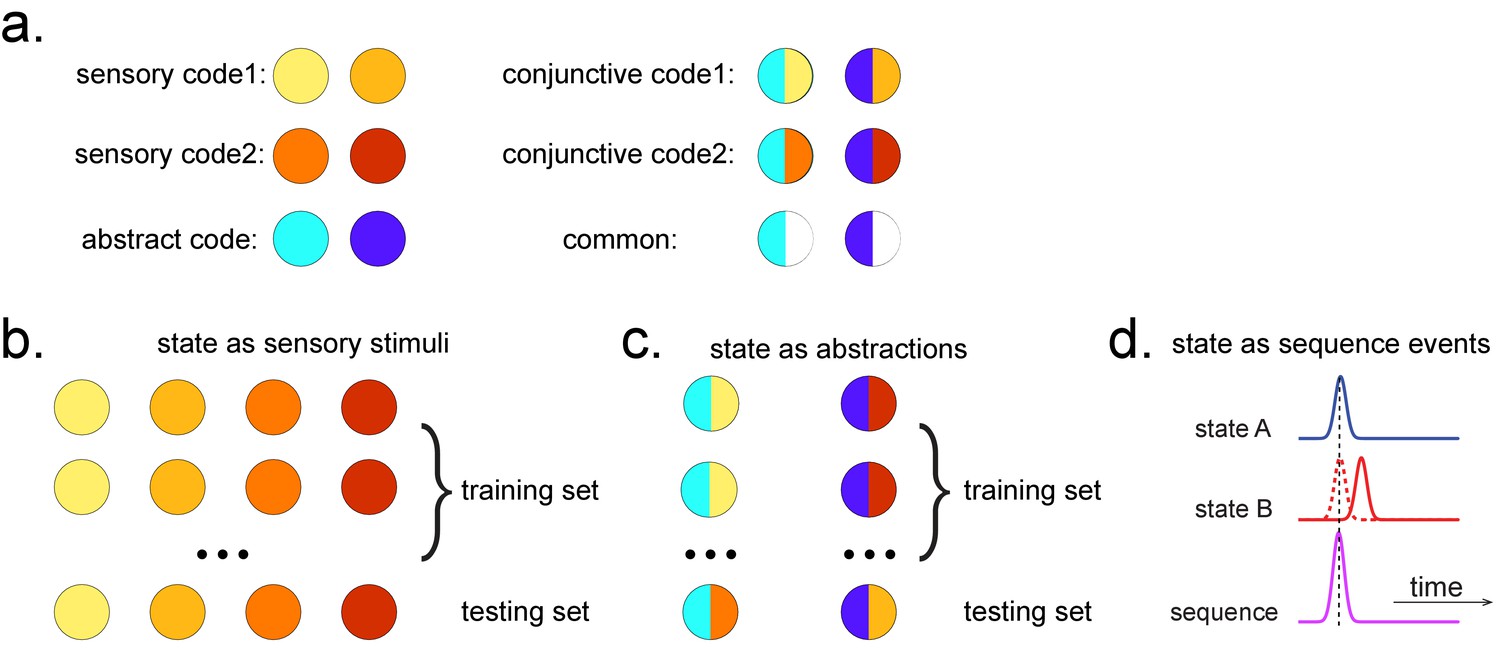
Obtaining different state spaces.
(a) Assuming we have two abstract codes, each abstract code has two different sensory codes (left panel). The MEG/EEG data corresponding to each stimulus is a conjunctive representation of sensory and abstract codes (right panel). The abstract code can be operationalized as the common information in the conjunctive codes of two stimuli. (b) Training decoding models for stimulus information. The simplest state is defined by sensory stimuli. To determine the best time point for classifier training, we can use a classical leave-one-out cross-validation scheme on the stimuli-evoked neural activity. (c) Training decoding models for abstracted information. The state can also be defined as the abstractions. To extract this information, we need to avoid a confound of sensory information. We can train the classifier on the neural activity evoked by one stimulus and test it on the other sharing the same abstract representation. If neural activity contains both a sensory and abstract code, then the only information that can generalize is the common abstract code. (d) The state can also be defined as the sequence event itself.
Figure 2—figure supplement 1
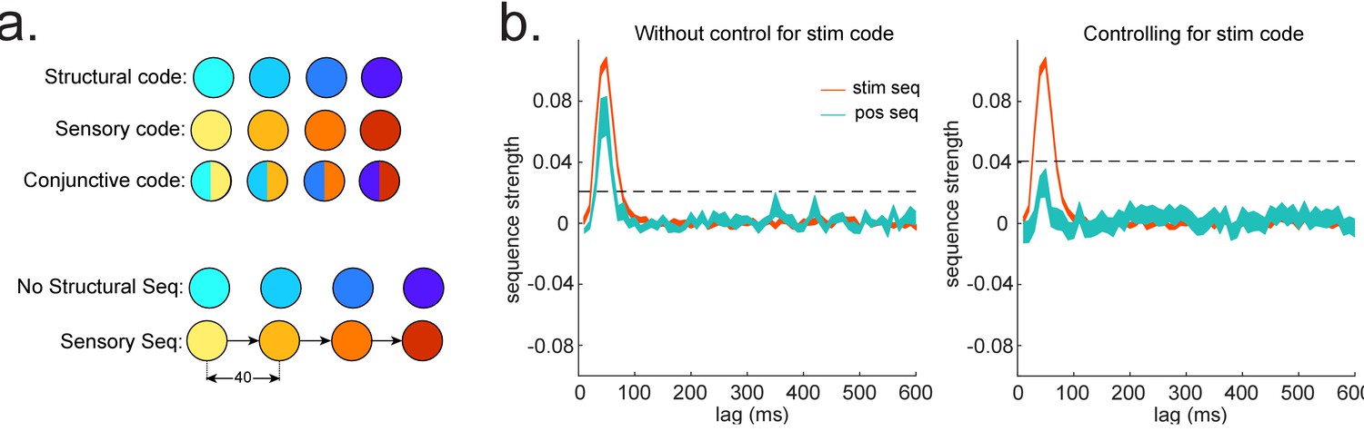
Sequences of abstract code.
(a) Illustration of the relationship between sensory code and (abstract) structural code. Structural code cannot be accessed directly but can be indirectly obtained from the conjunctive code (overlapping representation of sensory and structural code). In this simulation, there is sequence of sensory code but not of structural code. (b) We show the importance of controlling for sensory (stim) information when looking for sequences of abstract code: If sensory information is not controlled, we would observe significant sequences of structural code, while, in fact, it is not present, that is, false positive.
Figure 3
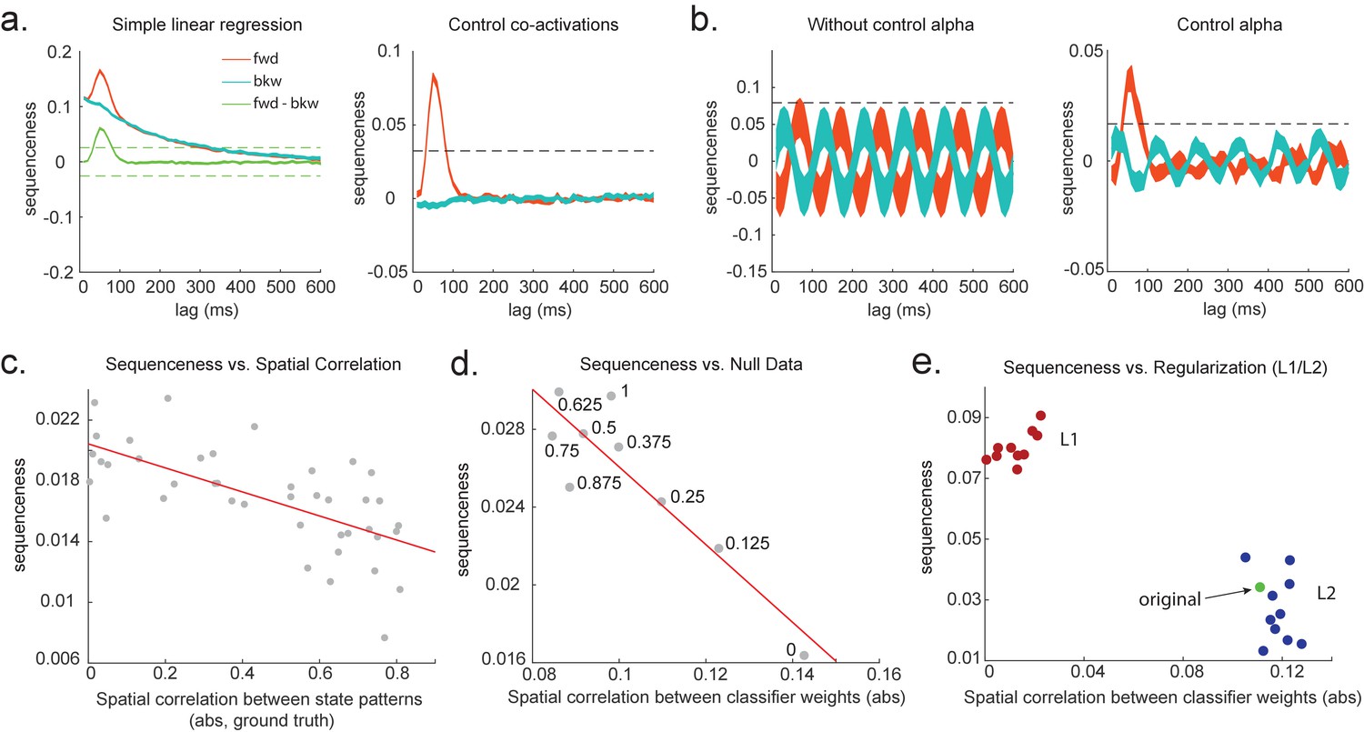
Effects of temporal, spatial correlations, and classifier regularization on temporal delayed linear modelling (TDLM).
(a) Simple linear regression or cross-correlation approach relies on an asymmetry of forward and backward transitions; therefore, subtraction is necessary (left panel). TDLM instead relies on multiple linear regression. TDLM can assess forward and backward transitions separately (right panel). (b) Background alpha oscillations, as seen during rest periods, can reduce sensitivity of sequence detection (left panel), and controlling alpha in TDLM helps recover the true signal (right panel). (c) The spatial correlation between the sensor weights of decoders for each state reduces the sensitivity of sequence detection. This suggests that reducing overlapping patterns between states is important for sequence analysis. (d) Adding null data to the training set increases the sensitivity of sequence detection by reducing the spatial correlations of the trained classifier weights. Here, the number indicates the ratio between null data and task data. ‘1’ means the same amount of null data and the task data. ‘0’ means no null data is added for training. (e) L1 regularization helps sequence detection by reducing spatial correlations (all red dots are L1 regularization with a varying parameter value), while L2 regularization does not help sequenceness (all blue dots are L2 regularization with a varying parameter value) as it does not reduce spatial correlations of the trained classifiers compared to the classifier trained without any regularization (green point).
Figure 4
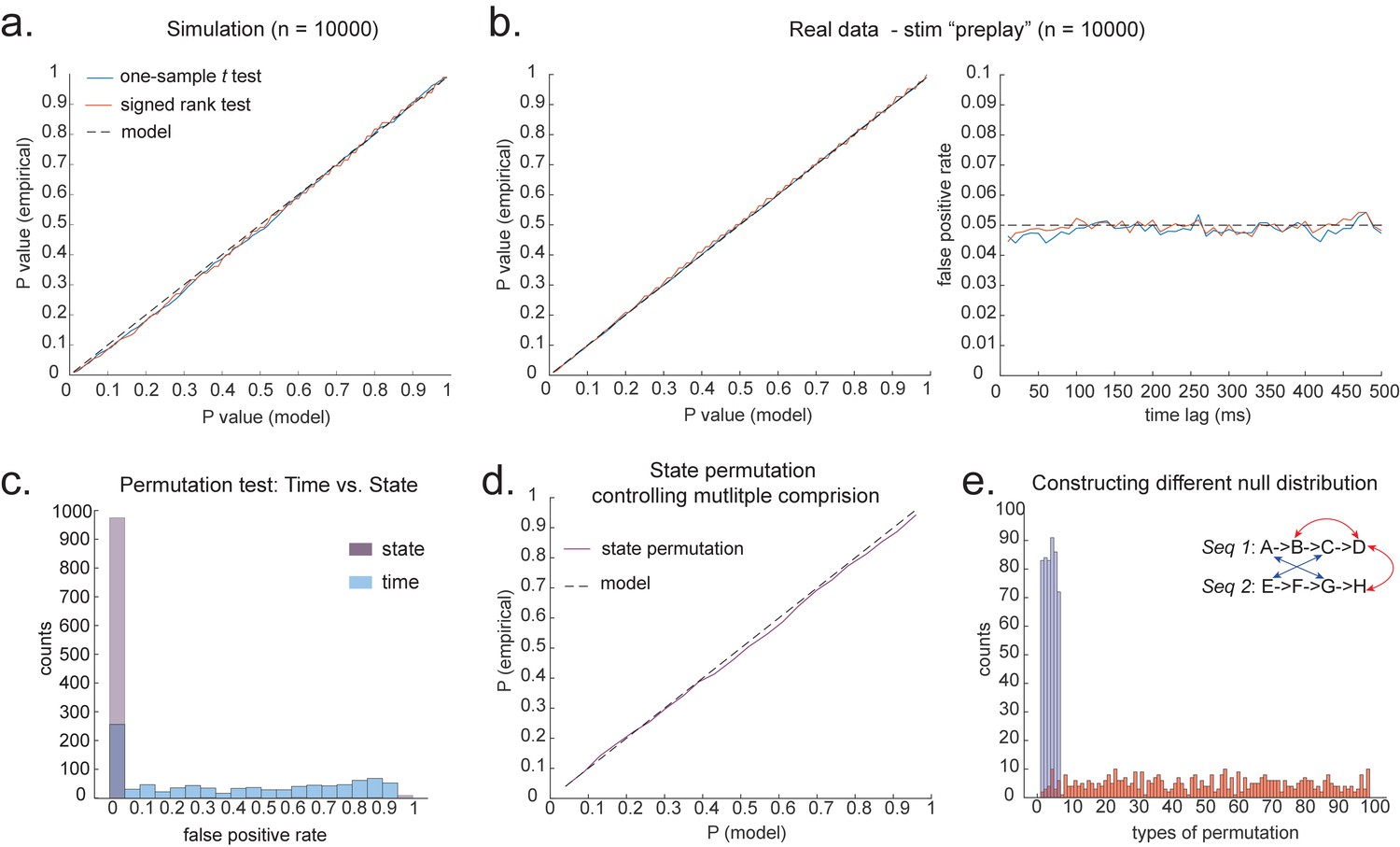
Statistical inference.
(a) P-P plot of one-sample t test (blue) and Wilcoxon signed-rank test (red) against zero. This is performed in simulated MEG data, assuming autocorrelated state time courses, but no real sequences. In each simulation, the statistics are done only on sequenceness at 40 ms time lag, across 24 simulated subjects. There are 10,000 simulations. (b) We have also tested the sequenceness distribution on real MEG data. Illustrated is the pre-task resting state on 22 subjects from Liu et al., where the ground truth is the absence of sequences given the stimuli have not yet been shown. The statistics are done on sequenceness at 40 ms time lag, across the 22 subjects. There are eight states. The state identity is randomly shuffled 10,000 times to construct a null distribution. (c) Time-based permutation test tends to result in high false positive, while state identity-based permutation does not. This is done in simulation assuming no real sequences (n = 1000). (d) P-P plot of state identity-based permutation test over peak sequenceness. To control for multiple comparisons, the null distribution is formed by taking the maximal absolute value over all computed time lags within a permutation, and the permutation threshold is defined as the 95% percentile over permutations. In simulation, we only compared the max sequence strength in the data to this permutation threshold. There are 10,000 simulations. In each simulation, there are 24 simulated subjects, with no real sequence. (e) In state identity-based permutation, we can test more specific hypotheses by controlling the null distribution. Blue are the permutations that only exchange state identity across sequences. Red are the permutations that permit all possible state identity permutations. 500 random state permutations are chosen from all possible ones. The X axis is the different combinations of the state permutation. It is sorted so that the cross-sequence permutations are in the beginning.
Figure 5
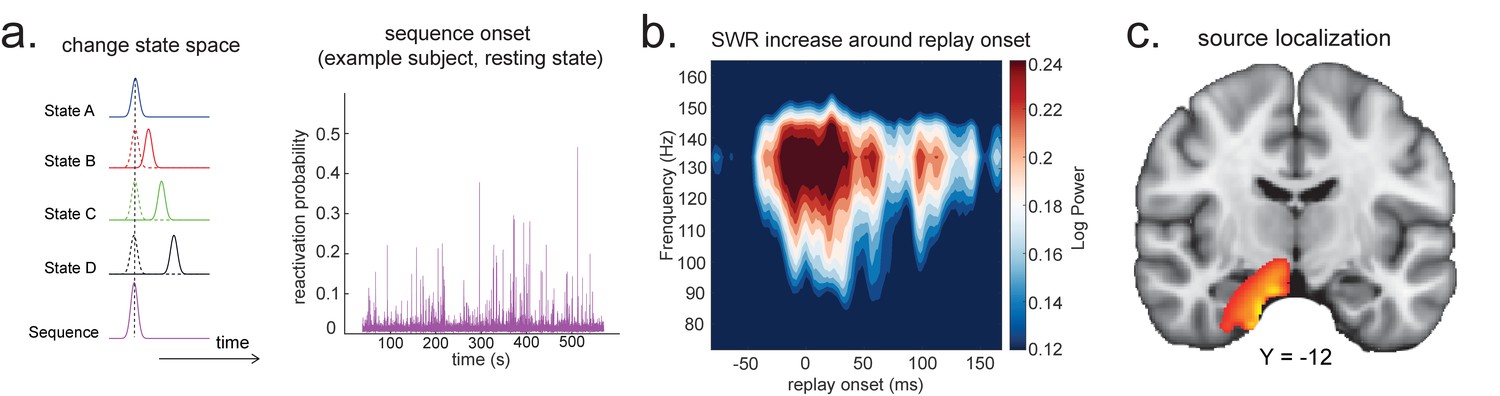
Source localization of replay onset.
(a) Temporal delayed linear modelling indexes the onset of a sequence based on the identified optimal state-to-state time lag (left panel). Sequence onset during resting state from one example subject is shown (right panel). (b) There was a significant power increase (averaged across all sensors) in the ripple frequency band (120–150 Hz) at the onset of replay compared to the pre-replay baseline (100 to 50 ms before replay). (c) Source localization of ripple-band power at replay onset revealed significant hippocampal activation (peak Montreal Neurological Institute, i.e., MNI coordinate: X = 18, Y = −12, Z = −27). Panels (b) and (c) are reproduced from Figure 7A, C, Liu et al., 2019, Cell, published under the Creative Commons Attribution 4.0 International Public License (CC BY 4.0).
Figure 6
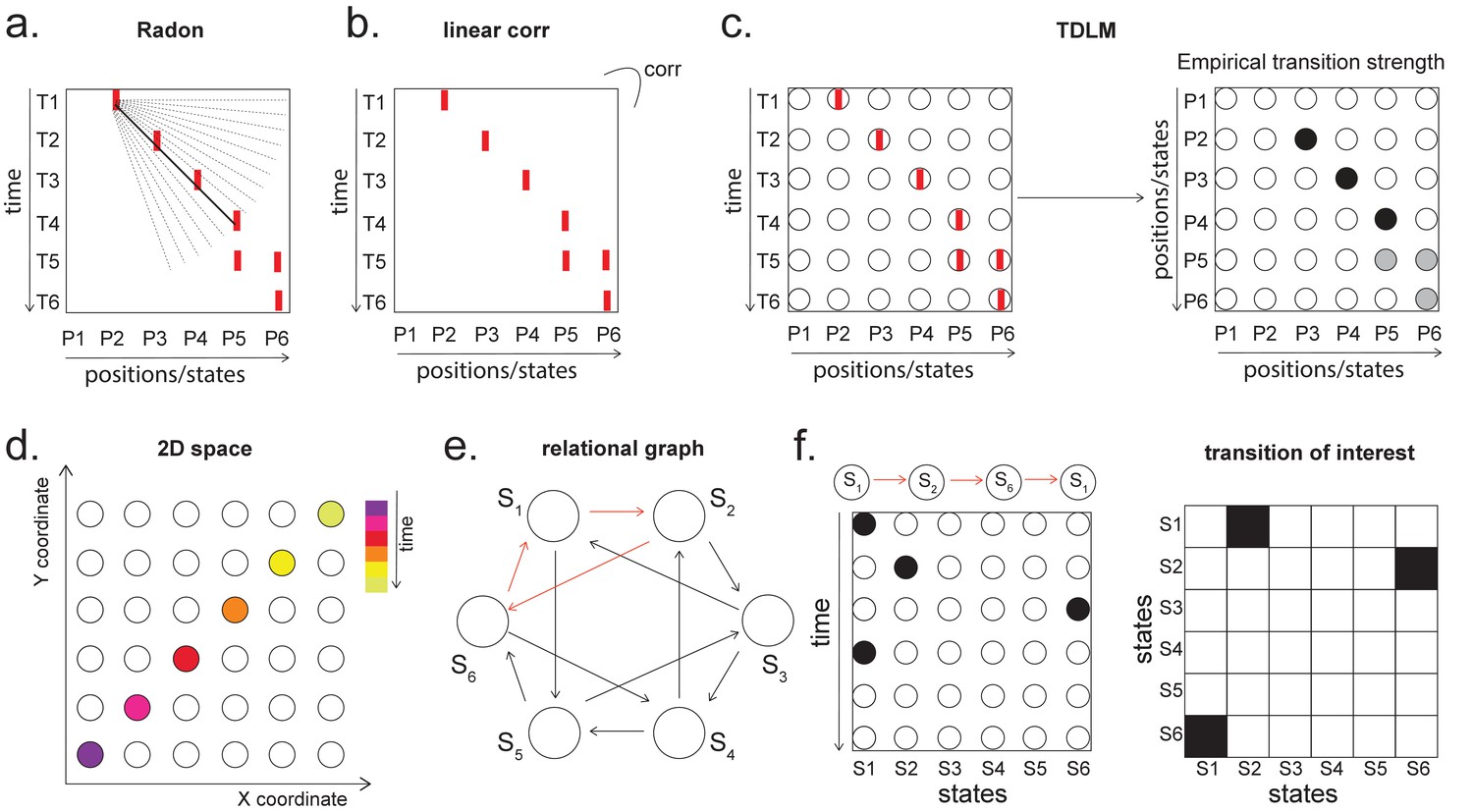
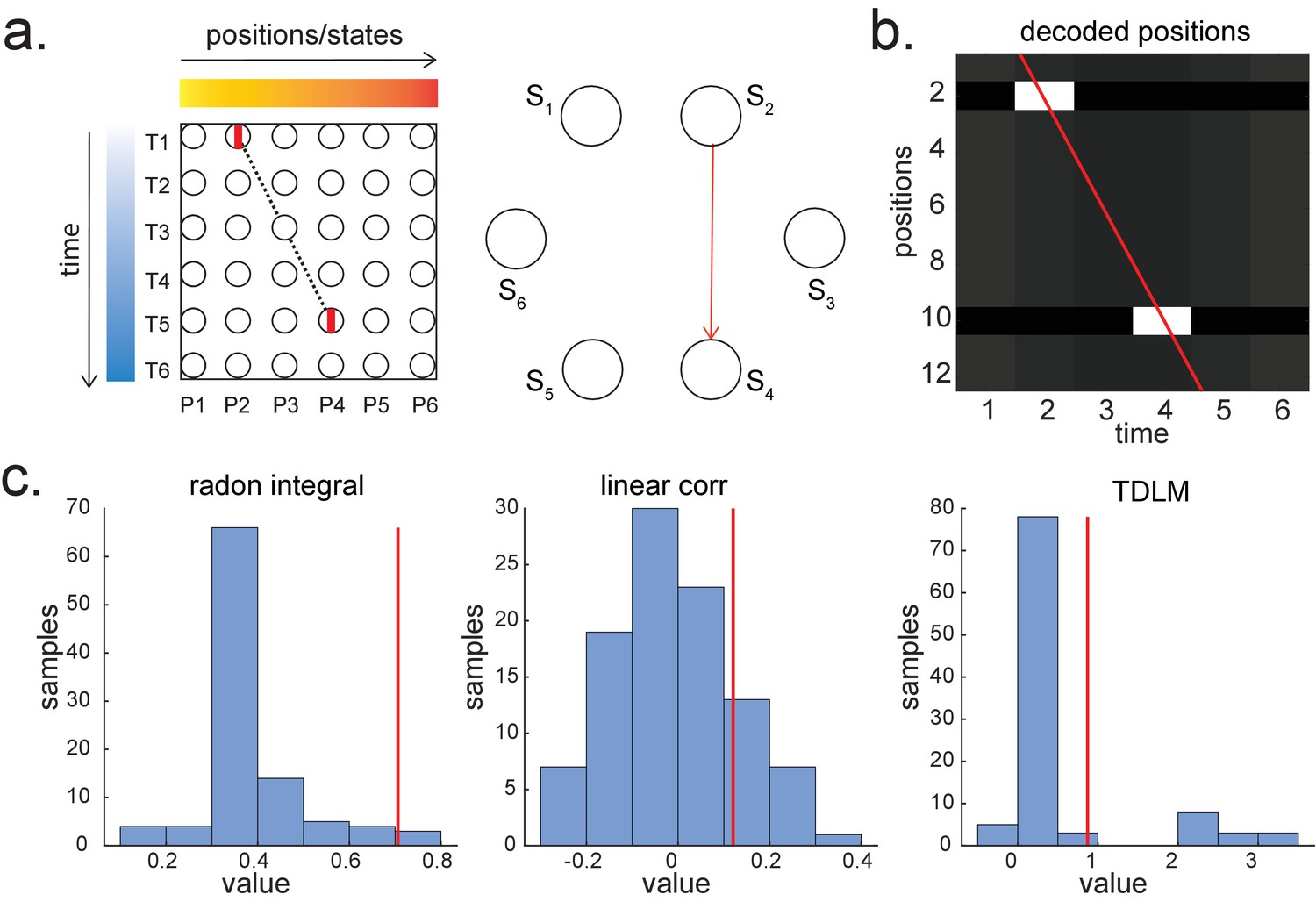
Temporal delayed linear modelling (TDLM) vs. existing rodent replay methods.
(a) The Radon method tries to find the best fitting line (solid line) of the decoded positions as a function of time. The red bars indicate strong reactivation at a given location. (b) The linear correlation method looks for correlations between time and decoded position. (c) The TDLM method, on the other hand, does not directly measure the relationship between state and time, but quantifies the likelihood of each transition. In the right panel, likelihood is indicated by darkness of shading. For example, P5 can be followed by either P5 or P6, making each transition half as likely as the deterministic P4->P5 transition. Later this empirical transition matrix is compared to a theoretical one, quantifying the extent to which the empirical transitions fit with a hypothesis. (d) Sequences in 2D space are in three dimensions, which is hard to translate into a line search problem, i.e., time*position spaces. (e) This is the transition matrix used in Kurth-Nelson et al., 2016, which cannot be translated into a linear state space. The transitions in red are an example of a trajectory. (f) Putting the example trajectory into the time by state matrix, we can see that there is no linear relationship between them (left panel). In TDLM, this is tested by forming a hypothesis regressor in the state-to-state transition matrix (right panel).
Figure 7
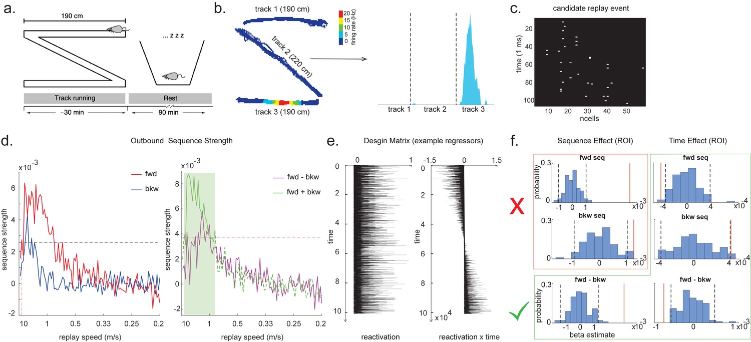
Temporal delayed linear modelling (TDLM) applied to real rodent data.
(a) The experimental design of Ólafsdóttir et al., 2016. Rats ran on Z maze for 30 min, followed by 90 min rest. (b) An example rate map for a place cell. The left panel shows its spatial distribution on the Z maze, and the right panel is its linearized distribution. (c) An example of a candidate replay event (spiking data). (d) Sequence strength as a function of replay speed is shown for the outbound rate map. Black dotted line is the permutation threshold after controlling for multiple comparisons. Left panel: forward sequence (red) and backward sequence (blue). The red dotted line indicates the fastest replay speed that is significant – 10 m/s. Right panel: forward–backward sequence. The pink dotted line indicates the multiple comparison-corrected permutation threshold for the replay difference. The green line is the sum of sequence strength between forward and backward direction. The solid line (with green shading) indicates the significant replay speeds (0.88–10 m/s) after controlling for multiple comparisons. We use this as a region of interest (ROI) to test for time-varying effect on replay in (f). (e) Illustration of two exemplar regressors in the design matrix for assessing time effect on replay strength. The ‘reactivation’ regressor is a lagged copy of reactivation strength of given position and is used to obtain sequence effect. The ‘reactivation × time’ regressor is the element-wise multiplication between this position reactivation and time (z-scored); it explicitly models the effect of time on sequence strength. Both regressors are demeaned. (f) Beta estimate of the sequence effect (left panel), as well as time modulation effect on sequence (right panel) in the ROI, is shown. Negative value indicates replay strength decreases over time, while positive value means replay increases as a function of sleep time. The statistical inference is done based on a permutation test. The two black dotted lines in each panel indicate the 2.5th and 97.5th percentile of the permutation samples, respectively. The red solid line indicates the true beta estimate of the effect. Note that there is a selection bias in performing statistical inference on forward and backward sequence strength (red rectangle) within this ROI, given the sum of forward and backward sequence is correlated with either forward or backward sequence alone. There is no selection bias in performing statistics on the difference of sequence effects or effects relating to time (green rectangle).
Figure 8
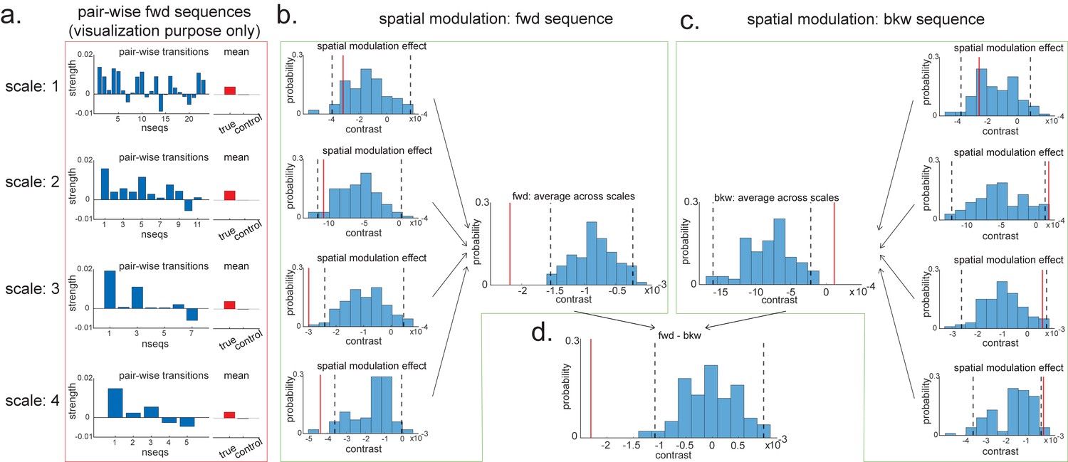
Pairwise sequence and spatial modulation effect.
(a) Within each scale, strengths of each pairwise forward sequences in the region of interest (ROI) (significant replay speeds, compare with Figure 7d, green shading) are ordered from the start of maze to the end of the maze; alongside that, the mean sequence strength across all of these valid pairwise transitions is plotted (red) in comparison to the mean of all control transitions (grey). This is for visualization purpose only and is included in the red rectangle. (b) The contrast defining a linear change in forward sequenceness across the track (spatial modulation) is shown (red line), both separately for each scale, and average across scales, and compared to permutations. On average, forward replay is stronger at the beginning of the track. (c) Same as panel (b), but this is for the backward sequences. Unlike forward replay, backward replay is stronger at the end of the track. Note that both panels (b) and (c) are about spatial modulation effect, which is orthogonal to overall sequence strength, allowing valid inference. They are therefore included in green boxes. (d) The difference of this spatial modulation effect between forward and backward sequence is also significant. The black dotted lines indicate the 2.5th and 97.5th percentile of the permutation samples. The red solid line indicates the estimate of the true contrast effect.
Appendix 1—figure 1
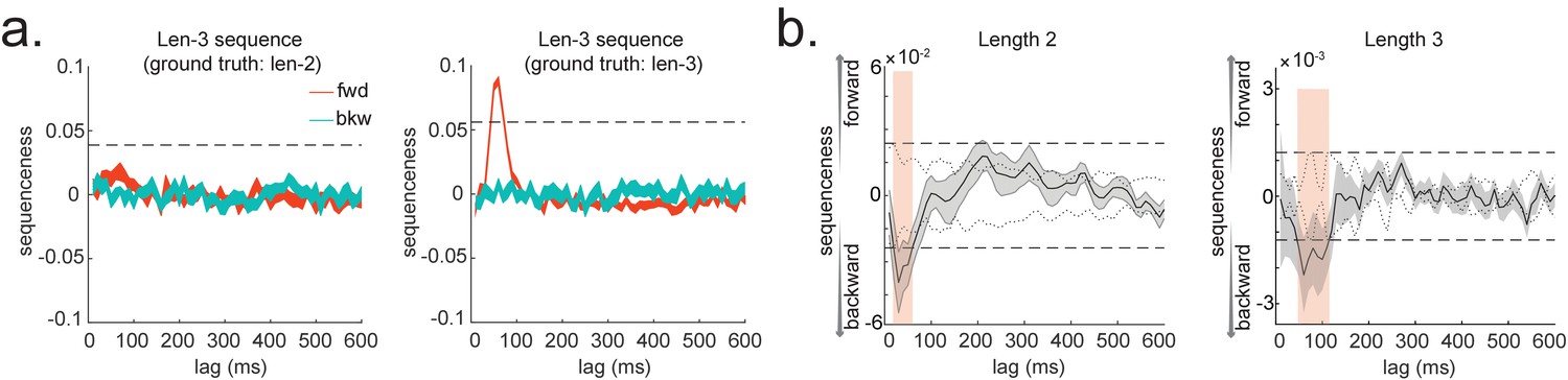
Extension to temporal delayed linear modelling (TDLM): multi-step sequences.
(a) TDLM can quantify not only pairwise transition, but also longer length sequences. It does so by controlling for evidence of shorter length to avoid false positives. (b) Method applied to human MEG data, incorporating control of both alpha oscillation and co-activation for length-2 and length-3 sequence length. Dashed line indicates the permutation threshold. This is reproduced from Figure 3A, C, Liu et al., 2019, Cell, published under the Creative Commons Attribution 4.0 International Public License (CC BY 4.0).
Appendix 3—figure 1

Sequences of sequences.
(a) Temporal delayed linear modelling (TDLM) can also be used iteratively to capture the repeating pattern of a sequence event itself. Illustration in the top panel describes the ground truth in the simulation. Intra-sequence temporal structure (left) and inter-sequence temporal structure (right) can be extracted simultaneously. (b) Temporal structure between and within different sequences. Illustration of two sequence types with different state-to-state time lag within sequence, and a systematic gap between the two types of sequences on top. TDLM can capture the temporal structures both within (left and middle panel) and between (right panel) the two sequence types.
Appendix 4—figure 1
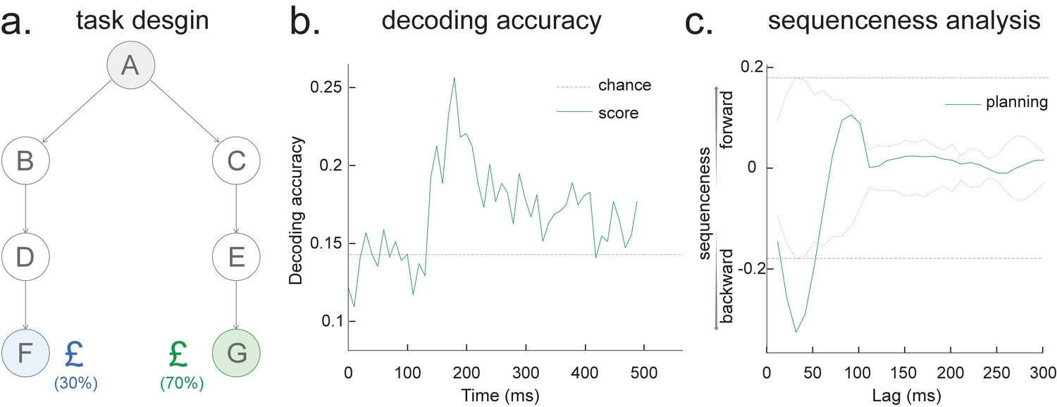
Sequence detection in EEG data (from one participant).
(a) Task design. At each trial, the participant starts at state A, and he/she needs to select either ‘BDF’ or ‘CEG’ path, based on the final reward receipt at terminal states F or G. All seven states are indexed by pictures. (b) The leave-one-out cross-validated decoding accuracy is shown, with a peak at around 200 ms after stimulus onset, similar to our previous MEG findings. (c) Temporal delayed linear modelling method is then applied on the decoded state time course where we find a fast backward sequenceness that conforms to task structure. Shown here is a subtraction between forward and backward sequenceness, where a negative sequenceness indicates stronger backward sequence replay. The dotted line is the peak of the absolute state permutation at each time lag, the dashed line the max over all computed state time lags, thereby controlling for multiple comparisons. This is the same statistical method used in our previous work and in the current paper. These EEG sequence results replicate our previous MEG-based findings at planning/decision time (see Figure 3 in Kurth-Nelson et al., 2016 and also see Figure 3f in Liu et al., 2019).
Appendix 5—figure 1
Parametric relationship between space and time vs. graph transitions.
(a) A scheme for skipping sequence (left). Both Radon and linear weighted correlation methods aim to capture a parametric relationship between space and time. Temporal delayed linear modelling (TDLM), on the other hand, tries to capture transitions in a graph (shown in right, with the red indicating the transition of interest). (b) A decoded time by position matrix from simulated spiking data. (c) Replay analysis using all three methods. TDLM is less sensitive compared to existing ‘line search’ methods, like radon or linear correlation. The red line indicates the true sequence measure from each of these methods. The bar plots are permutation samples by randomly shuffling the rate maps.
Author response image 1

Illustration of three replay detection methods on the decoded time by position/state spaces.
a. The Radon method tries to find the best fitting line (solid line) of the decoded positions as a function of time. The red bars indicate strong reactivation at given locations. b. The linear correlation method tests for a correlation between time and decoded position. c. The TDLM method on the other hand, does not directly measure relationship between state and time, but quantifies the strength of evidence for each possible transition, indicated by the solid black/grey dots, where the colour gradient indicates transition strength. For example, P5→P6 is lighter than P4→P5, this is because following reactivation of P5 in time T4, both P5 and P6 are reactivated at the same time – T5. Later this empirical transition matrix is compared to a theorical/ hypothesised one, to quantify the extent to which the empirical transitions fit with an experimental hypothesis.
Author response image 2
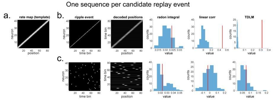
"line search” approach vs. TDLM on the simulated spiking data (assuming single ground-truth sequence).
(a) The rate map of the simulated place cells (n=40) over a linearized space with 80 positions. It is smoothed with 2 sample gaussian kernel, to mimic overlapping place fields. (b) We simulated a ground truth sequence with time lag of 2 time samples between successive firings in the ripple event. The histogram is the sequence distribution of the shuffled data (in blue). The red line is the sequence results for the true data. The permutation is done by shuffling the rate map of each cell, so that the place fields are randomized. (c) We randomly shuffled the firing order in the ripple event, so that there is no structured sequence in the simulation. We show that all methods report non-significant evidence of sequenceness.
Author response image 3

“line search” approach vs. TDLM on the simulated spiking data (assuming two ground-truth sequences).
(a) The rate map of the simulated place cells (n=40) over a linearized space with 80 positions, smoothed with 2 sample gaussian kernel, to mimic overlapping place fields. (b) We simulated two ground truth sequences with time lag of 2 time samples between successive firings in the ripple event. We also show the decoded position space right next to the ripple event. All replay analyses are performed on this decoded space. The histogram is the sequence distribution of the shuffled data (in blue). The red line is the sequence results in the true data. (c) We randomly shuffled the firing order in the ripple event, so that there are no structured sequences in the simulation. We show there is no temporal structure in the decoded position space. As a result, TDLM reports no significant sequenceness value on the decoded position space.
Author response image 4
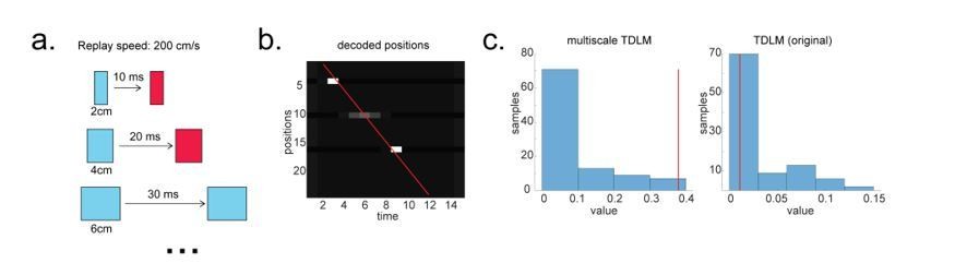
Multi-scale TDLM.
(a) Illustration of a change in state space for the same replay speed. (b) A possible scenario for the application of multi-scale TDLM, where only subsets of state on a path were reactivated. The red line is the best linear fit based on Radon method. (c) TDLM method. TDLM with multi-scaling is more sensitive than TDLM in the original state space and reports significant sequenceness.
Author response image 5

TDLM applied to real rodent data.
(A) Sequence strength as a function of speed and direction is shown for outbound rate map. Dotted line is the permutation threshold. We have both significant forward (blue) and backward (red) sequence with peak speed around 167 – 333 cm/s. (B) Sequence strength for an inbound rate map is shown. (C) Sequence strength estimated separately for early, middle and late sleep time, also for inbound, outbound rate map. There are more replays in the early sleep time than middle or late, especially in the speed range of 100-500 cm/s. Dotted line is the permutation threshold.
Author response image 6
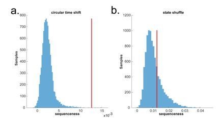
Circular time shift vs. state identity-based permutation on real human whole brain MEG data.
(a) The permutation (blue) is done by circularly shifting the time dimension of each state on the decoded state space of the MEG data during pre-stimuli resting time, where the ground truth is no sequence. There is a false positive. (b) The permutation (blue) is done by randomly shuffling the state identity. There is no false positive.
Additional files
Download links
A two-part list of links to download the article, or parts of the article, in various formats.
Downloads (link to download the article as PDF)
Open citations (links to open the citations from this article in various online reference manager services)
Cite this article (links to download the citations from this article in formats compatible with various reference manager tools)
Temporally delayed linear modelling (TDLM) measures replay in both animals and humans
eLife 10:e66917.
https://doi.org/10.7554/eLife.66917


