Environmental fluctuations reshape an unexpected diversity-disturbance relationship in a microbial community
- Department of Biomedical Engineering and Biological Design Center, Boston University, United States
- Department of Physics, Massachusetts Institute of Technology, United States
- Wyss Institute for Biologically Inspired Engineering, Harvard University, United States
Figures
Figure 1
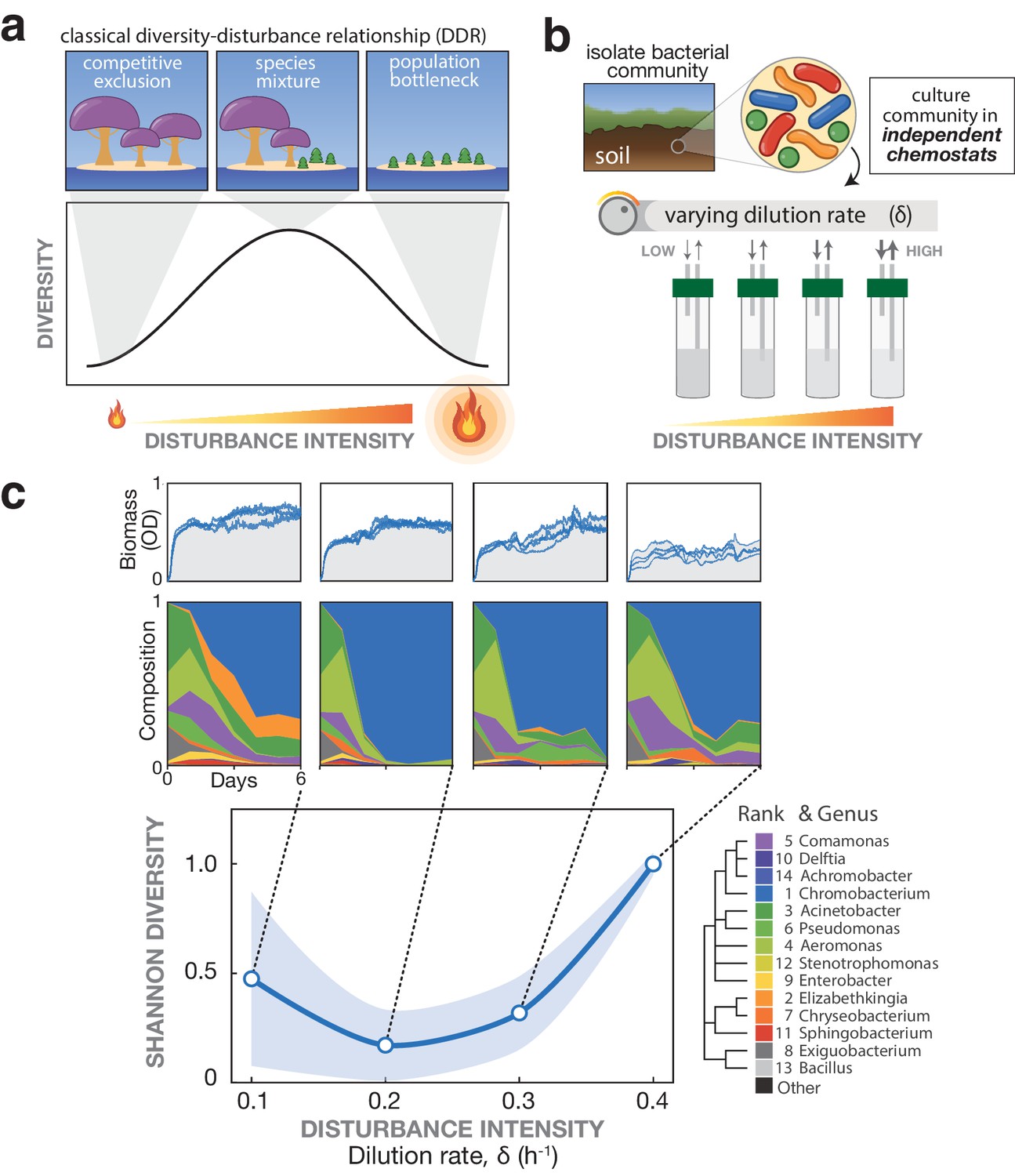
Emergence of a U-shaped diversity-disturbance relationship (DDR) in a microbial community for constantly applied disturbance at different intensities.
(a) Different DDRs have been proposed based on observations of natural ecosystems, including the Intermediate Disturbance Hypothesis in which diversity peaks at intermediate disturbance levels, see depiction. (b) In the laboratory, microbial communities can be cultivated and subjected to varying disturbance intensity levels by tuning the dilution rate in chemostats. (c) A bacterial community exhibits a U-shaped diversity dependence on the disturbance intensity. Samples of a soil-derived bacterial community were grown for 6 days in eVOLVER mini-chemostats at four different dilution rates. Top: Optical density over time quantifies biomass for replicate cultures. Middle: Mean relative abundance of bacterial genera from replicate cultures, determined by 16S sequencing. Mean rank abundance is denoted by order, taxonomic similarity is denoted by color. Bottom: Plotting the endpoint number of species (Amplicon Sequence Variants) vs. dilution rate produces a U-shaped curve, rather than a peaked DDR. Shaded window indicates a one standard deviation confidence interval.
Figure 2 with 1 supplement
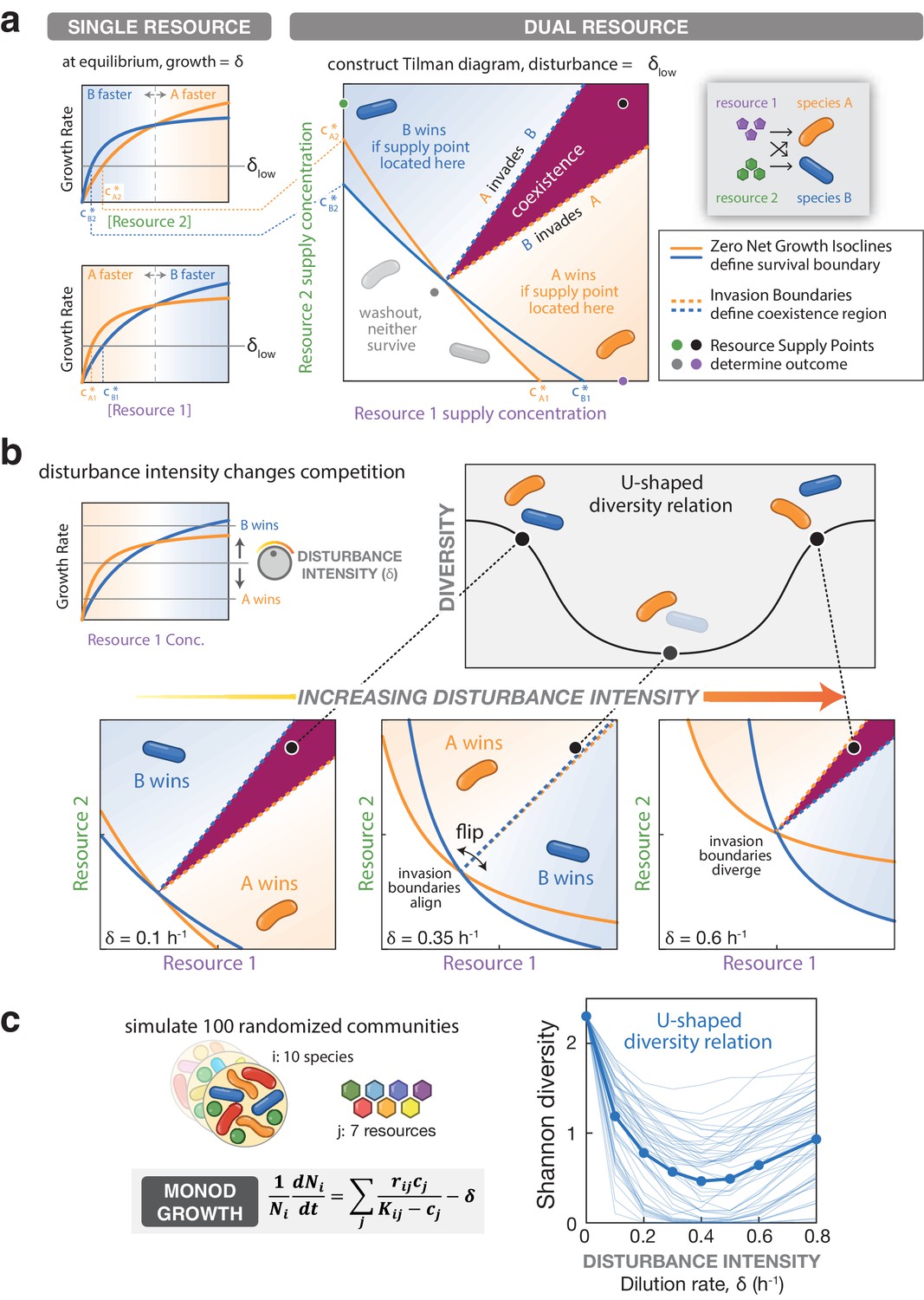
A U-shaped diversity disturbance relationship can emerge from a consumer resource model if species undergo niche-flip as disturbance increases.
(a) The survival of a species in a consumer resource model depends on the supplied resource levels and the mortality rate (i.e. disturbance intensity). A Zero Net Growth Isocline (ZNGI) may be defined for each species at a given disturbance intensity, delineating the range of resource supply levels where growth can meet or exceed the mortality rate. The ZNGIs intersect the axis at c* values, the minimum concentration needed to support growth of a species on a single resource. The outcome of competition depends on the combination of resources supplied, indicated by a supply point. Resources are consumed until reaching equilibrium along the ZNGI of the species requiring the fewest resources to survive at the specified mortality rate, the winner of the competition. Different supply points can be found that support neither species (gray), a single species (green or purple) or both species (black). Invasion boundaries indicate regions where one species can increase in density in the presence of the other, outlining the region of coexistence (maroon). (b) In a consumer resource simulation with 2-species / 2-resources and Monod growth, the outcome of competition at the given supply point (black) depends on disturbance intensity. Both ZNGIs and invasion boundaries flip as disturbance intensity increases. At intermediate disturbance, invasion boundaries align and the coexistence region collapses, reducing diversity relative to low/high disturbance intensities at the black supply point. (c) Left: Monod consumer resource model for growth of species i with additive non-linear growth on each resource. Right: Shannon diversity of randomly generated 10-species communities, after six days of simulated growth on seven resources at varying dilution rates. For each model, mean diversity was computed for 100 randomly initialized communities, across each mean dilution rate, 50 of which are shown as individual traces.
Figure 2—figure supplement 1
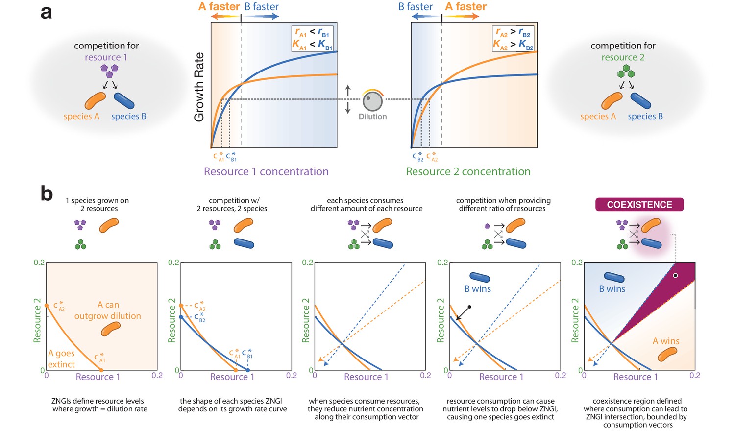
Navigating between Monod growth curves and Tilman diagrams.
Growth rates calculated using consumer resource models can be used to construct diagrams of competitive outcomes, see Tilman, 1982. (a) Consider Species A and Species B, which each exhibit different resource concentration-dependent growth on Resource 1 or Resource 2. To achieve growth rates equal to this indicated dilution rate, the species require different resource concentrations to survive, called c* values. (b) In a multi-resource environment, the summed growth rate across resources constructs a Zero Net Growth Isocline (ZNGI) which intersects the axes at c* points from the prior panel. ZNGIs define the space of supplied resource that can support a species sufficiently such that its growth meets or exceeds the mortality rate (e.g. dilution rate). The outcome of competition can be predicted by determining whether resource consumption will drive one species to extinction or not. The borders of these different outcomes, termed invasion boundaries in Figure 2, can be identified by calculating a resource consumption vector at the intersection of the ZNGIs. Note that Tilman diagrams may be constructed for any consumer resource model, and the shapes and movement of the ZNGIs will change accordingly.
Figure 3 with 13 supplements
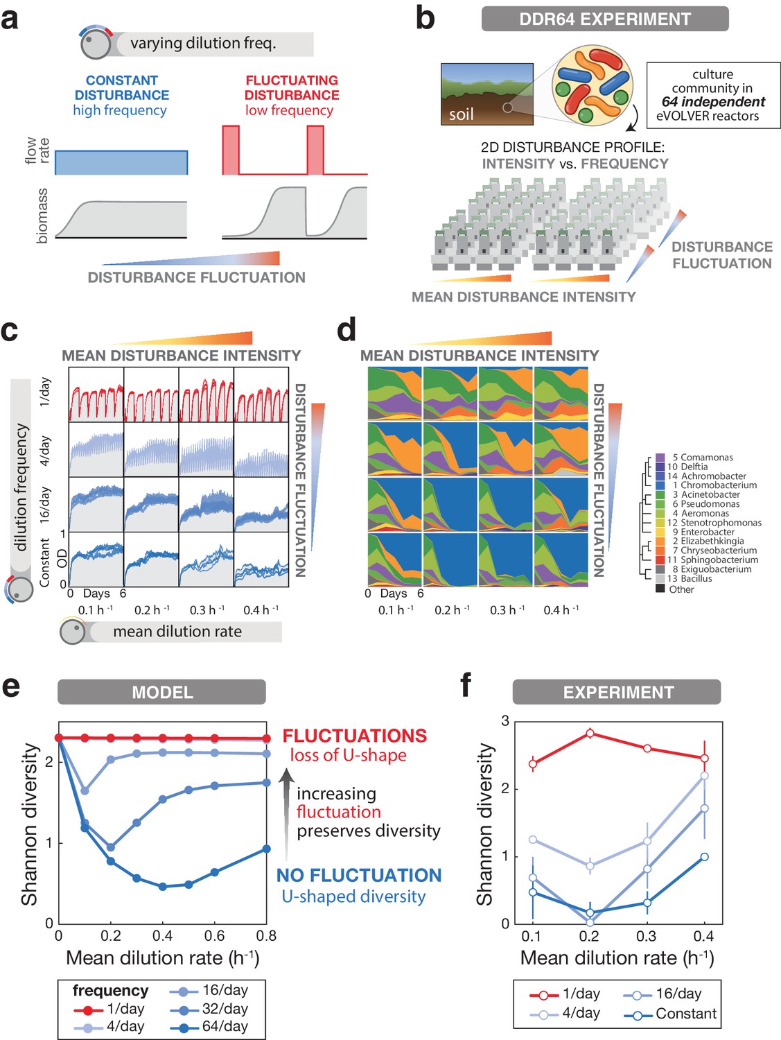
Introducing environmental fluctuations reshapes DDR and increases diversity levels in a microbial community.
(a) Fluctuations in a disturbance over time cause fluctuations in biomass, and can be varied independently of the disturbance intensity. In continuous culture, fluctuations are achieved by aggregating dilution into discrete events while keeping mean dilution rate constant per day. (b) Schematic of the eVOLVER DDR64 experiment in which disturbance components (intensity and fluctuation) are varied independently. Samples of a soil-derived bacterial community were continuously cultured for 6 days across 64 eVOLVER bioreactors with varying mean dilution rate and dilution frequency. (c) Optical density traces for culture replicates in each condition show the dependence of biomass on disturbance. (d) Mean relative abundance of bacterial genera from replicate cultures, determined by 16S sequencing. Mean rank abundance is denoted by order, taxonomic similarity is denoted by color (see legend). (e) Mean Shannon diversity across 100 Monod consumer resource model simulations with varying mean dilution rate and dilution frequency show that the dependence of diversity on disturbance is fluctuation-dependent. (f) Mean Shannon diversity of Amplicon Sequence Variants from the DDR64 experiment vs. mean dilution rate and dilution frequencies. As in the simulations, fluctuations increase diversity and eliminate the U-shape. Bars in e and f denote standard error of the mean.
-
Figure 3—source data 1
Population size and diversity metrics for DDR64 and DDR washout.
- https://cdn.elifesciences.org/articles/67175/elife-67175-fig3-data1-v2.csv
-
Figure 3—source data 2
Genus level composition for DDR64 and DDR washout.
- https://cdn.elifesciences.org/articles/67175/elife-67175-fig3-data2-v2.csv
Figure 3—figure supplement 1
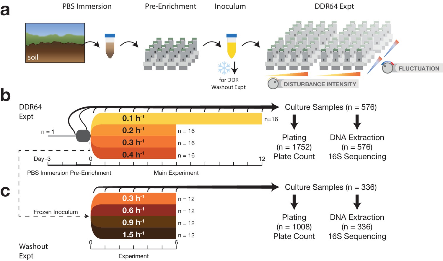
Timeline of DDR64 and DDR washout experiments.
(a) Soil samples were immersed in PBS, then pre-enriched in overnight cultures in 0.1X Nutrient Broth. Post-enrichment cultures were mixed to form the final inoculum. The final inoculum was also frozen for follow-up experiments. (b) Timeline for the DDR64 Experiment. Cultures were sampled daily for plating and sequencing to determine composition. Cultures completed ~20–90 generations over 6 days. The 0.1 h−1 cultures were carried out for an additional 6 days in order to complete an additional 20 generations, for a total of 40. (c) Timeline and sampling schedule for DDR Washout Experiment. This experiment was started from a frozen sample of the inoculum used in the DDR64 experiment.
Figure 3—figure supplement 2
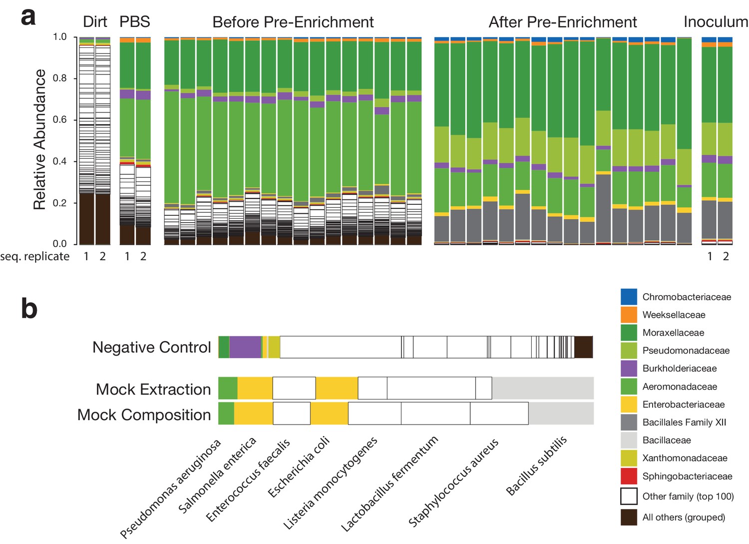
Inoculum composition determined by 16S sequencing.
(a) Family-level composition of a representative soil sample, supernatant of PBS immersion, pre-enrichment cultures, and final inoculum. Diversity and composition changes over time indicate selection for growth in lab conditions. (b) Composition of negative control sample, positive control mock community sample, and the true composition of the mock community sample. Positive control samples indicate coverage over both Gram-positive and Gram-negative organisms. Negative control sample indicates that the composition of experimental samples is significantly different, as would be expected for samples of sufficient biomass.
Figure 3—figure supplement 3
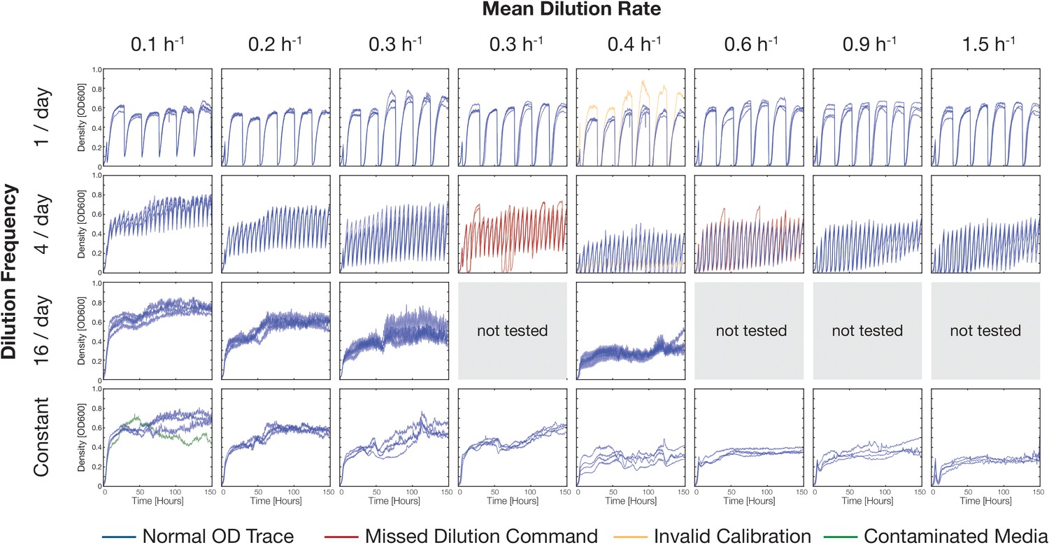
Optical density over time for DDR64 and DDR washout experiments.
Optical density was recorded in each eVOLVER vial over time at ~30 s intervals. Plots from vials in replicate conditions are included on the same axes. Colors used to indicate technical issues in that vial. DDR64 experiment located in columns 1,2,3,5; DDR Washout experiment in columns 4,6,7,8.
Figure 3—figure supplement 4
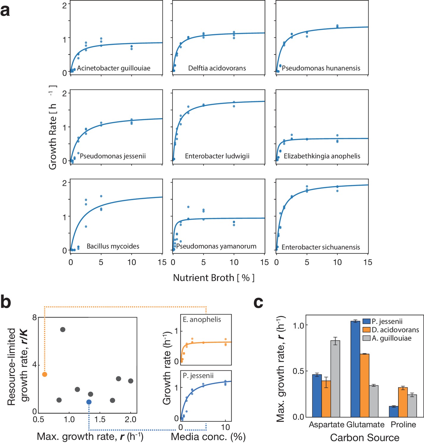
Measured growth of isolates in Nutrient Broth indicate variation in r and K parameters across different medias.
(a) Nine isolates from the DDR64 and DDR Washout experiments were grown in a microplate spectrophotometer in dilute Nutrient Broth media (ranging from 0.1X to <0.0016X, plus a water-only negative control). Linear regression on a Lineweaver-Burk plot was used to calculate Monod and values. Monod curves generated from those fit values are indicated by solid lines, while triplicate growth measurements are indicated as points. Flattening of growth rate vs. nutrient concentration curves is consistent with saturating growth in Monod model. (b) Scatter plot of Monod and values indicate that while species vary in Monod and , these values are uncorrelated. If there were a strong positive correlation between and , this would prevent a U-shaped DDR according to the model. (c) Three isolates from the DDR64 and DDR Washout experiments were grown in M9 media supplemented with 10mM of the indicated amino acid as a sole carbon source. Different isolates had different growth rates on each resource, indicating resource preferences.
Figure 3—figure supplement 5

Species richness from Monod Consumer Resource model exhibits U-shaped DDRs.
Each plot displays species richness after 6 days of simulated growth, mean across 100 communities for varying mean dilution rate and dilution frequency (see legend). Variations on the basic Monod model are discussed in Materials and methods. Richness was defined as the number of species with abundances above the indicated population size threshold at the simulation endpoint. The U-shaped DDR is more distinct at higher thresholds.
Figure 3—figure supplement 6
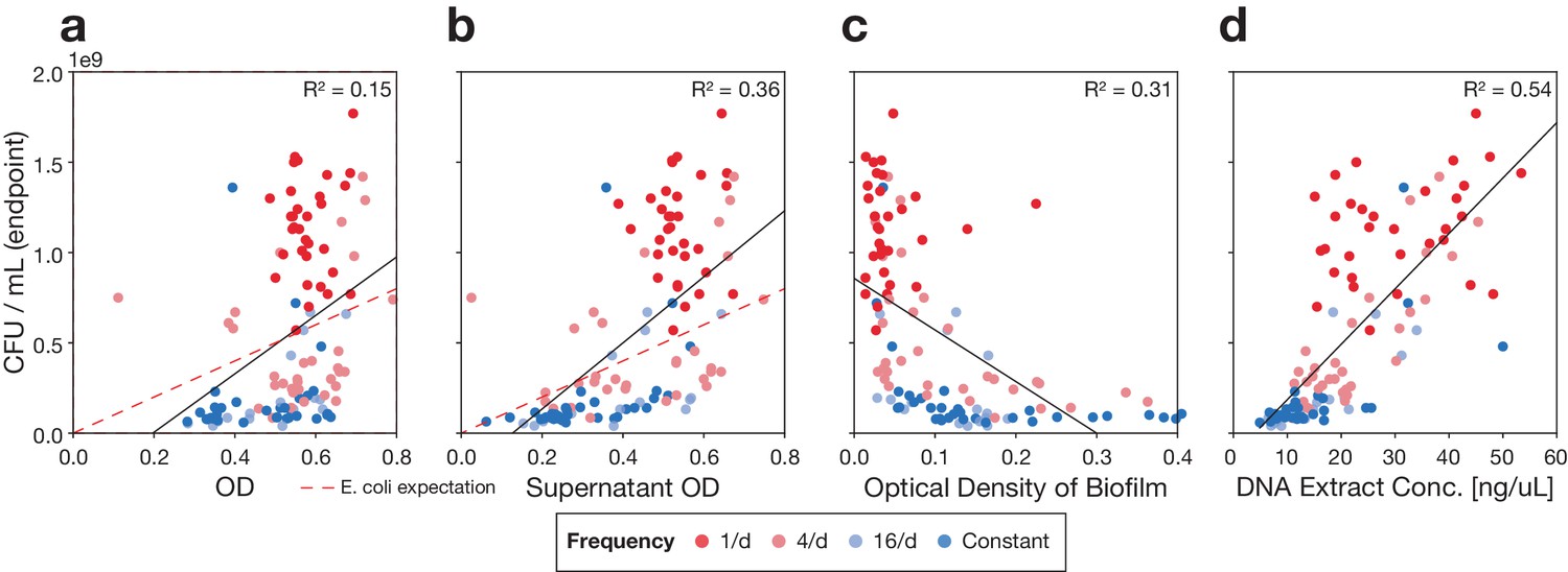
Correlation between population size estimates vary according to condition and biofilm accumulation.
Colony forming units (CFU) for endpoint samples plotted against other population size estimates. (a) CFU/mL vs. Optical Density in eVOLVER. (b) CFU/mL vs. Optical Density in eVOLVER, minus biofilm contribution. (c) CFU/mL vs. Optical Density of biofilm (see Figure 3—figure supplement 12). (d) CFU/mL vs. concentration yield of DNA extraction. For all plots, linear regression line is plotted in black, with corresponding R2 values. For optical density plots, a linear relationship (CFU/OD = 8 x 10⁸) color indicates frequency of dilution (see legend). Samples in the 1/d condition group were measured to have much higher CFU/mL, as these cultures reached saturation.
Figure 3—figure supplement 7
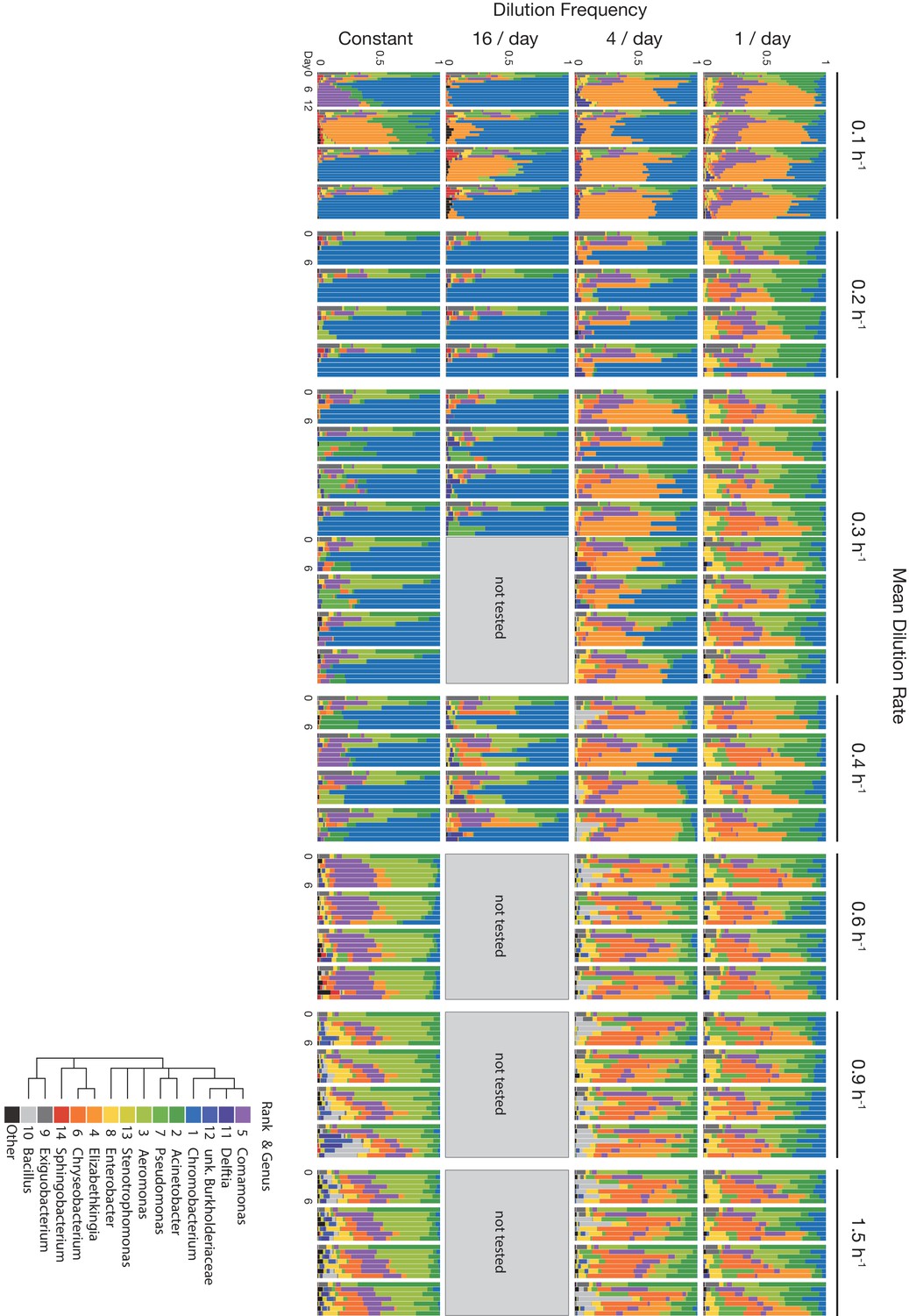
Genus-level composition over time in the DDR64 and DDR Washout experiments.
Composition was determined to vary over time across different disturbance intensity and fluctuation levels. Daily samples were taken from soil microbe co-cultures grown in eVOLVER in varying dilution profiles (Materials and methods). Amplicon sequencing on the v4 16S region was performed and analyzed in QIIME 2 to assign genus level taxonomy according to the SILVA 132 database. Each bar depicts the relative abundance of genera in a single sample. Mean rank abundance of a bacterial genus (across all samples) is denoted by order (top to bottom), and taxonomic similarity is denoted by color (see legend).
Figure 3—figure supplement 8
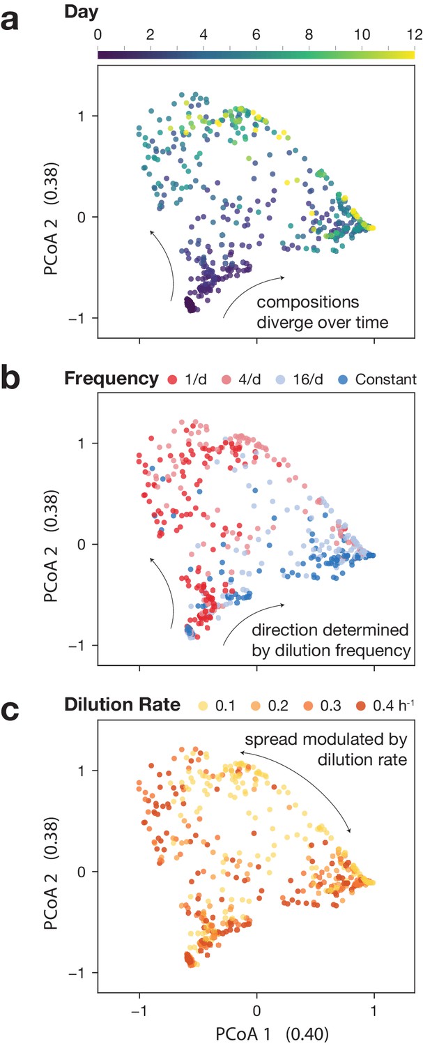
Principle coordinate analysis shows varying composition in DDR64 experiment.
Principal coordinate analysis indicates divergence in composition between samples. Ordination was based on Weighted UniFrac distances that were calculated from 16S composition of daily samples in QIIME 2. (a) Samples colored according to day of collection. (b) Samples colored to indicate the dilution frequency of the culture. (c) Samples colored to indicate the mean dilution rate of the culture. The magnitude for each principle coordinate is listed in parentheses.
Figure 3—figure supplement 9
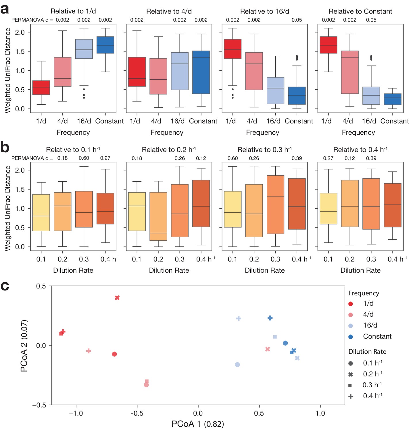
PERMANOVA analysis shows disturbance frequency significantly affects composition.
Ordination was based on Weighted UniFrac distances that were calculated from 16S composition of Day 6 samples only in QIIME 2. PERMANOVA testing was used to determine whether distances between cultures grouped by disturbance characteristics were statistically significant. The PERMANOVA significance values (corrected for false discovery rate) are provided above each pair, with q<0.05 being a significant result. (a) Pairwise distances between cultures grouped by the disturbance frequency under which they were grown. Significant differences exist between low-frequency and high-frequency cultures. (b) Pairwise distances between cultures grouped by the mean dilution rate under which they were grown. (c) Principal coordinate analysis of mean composition at Day 6 for the 16 different dilution rate-frequency combinations indicates the contributions of dilution rate and frequency to composition differences. No pairwise distances between dilution rate-frequency combinations were significant by PERMANOVA after correction for false discovery rate from multiple hypotheses (lowest q=0.067), though numerous pairwise distances were found to have p<0.05.
Figure 3—figure supplement 10
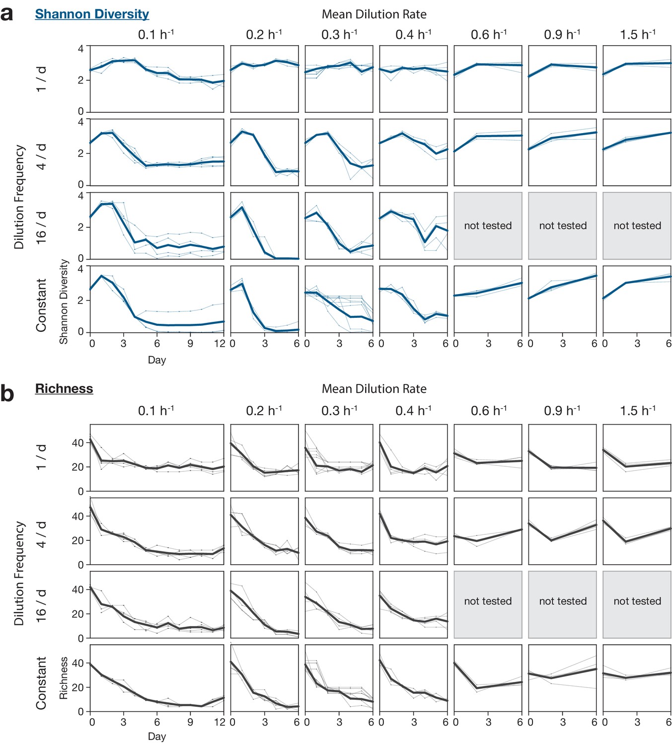
Diversity changes over time in DDR64 and DDR washout experiments.
Diversity was calculated from 16S sequencing for each timepoint sample in each vial. (a) The Shannon diversity of 16S ASVs for each vial are indicated by points connected by thin lines. The mean across replicate vials is denoted with a thick line. (b) 16S ASV richness for each vial, plotted as above. Samples with technical issues (e.g. poor sequencing coverage, contamination, see Figure 3—figure supplement 3) were excluded from analysis.
Figure 3—figure supplement 11
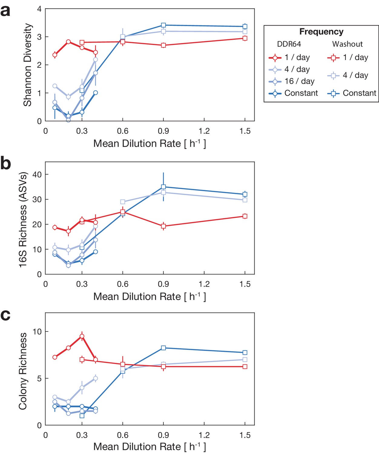
Different diversity metrics from DDR64 and DDR washout experiments show U-shaped DDRs.
Diversity was calculated using the Day 6 timepoint for all vials in DDR64 and DDR Washout experiments. (a) Shannon diversity of 16S ASVs for each vial, mean across replicates. (b) 16S ASV richness for each vial, mean across replicates. (c) Colony richness, the number of unique colony morphotypes identified on Nutrient Agar plate for each vial, mean across replicates. Note that due to CFU/mL differences, colony richness is deflated in low-density conditions. This effect is pronounced in the constant dilution vials. Bars indicate standard error of the mean. Samples with technical issues (e.g. poor sequencing coverage, contamination, see Figure 3—figure supplement 3) were excluded from analysis.
Figure 3—figure supplement 12

Heatmap of biofilm levels at endpoint.
Biofilm levels were measured by flushing vials with fresh media then measuring optical density in eVOLVER. Vials with higher optical density have more biofilm accumulation. Heatmap depicts mean across replicates. DDR64 experiment data in columns 1,2,3,5 and DDR Washout experiment in columns 4,6,7,8.
Figure 3—figure supplement 13
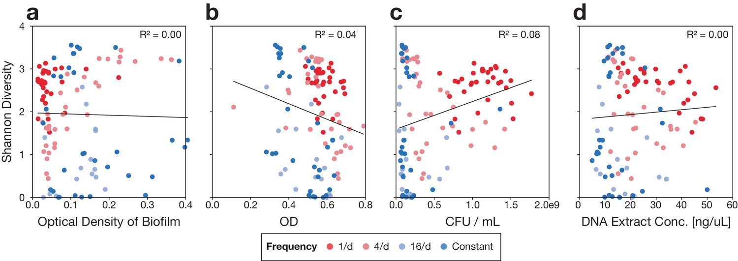
Diversity does not correlate with potential confounding factors.
Shannon diversity of 16S ASVs for endpoint samples plotted against potential confounding factors. (a) Diversity vs. Optical Density of biofilm (see Figure 3—figure supplement 12). (b) Diversity vs. Optical Density in eVOLVER. (c) Diversity vs. CFU/mL calculated from Nutrient Agar plate. (d) Diversity vs. concentration yield of DNA extraction. For all plots, a linear regression line is plotted in black, with corresponding R2 values. Color indicates frequency of dilution (see legend).
Figure 4

Distinct classes of diversity-disturbance relationships emerge when traversing different regions of disturbance (intensity vs. fluctuation) space.
A simple Monod consumer resource model maps a phase diagram for community diversity by varying distinct characteristics of environmental disturbance (intensity and fluctuation). Diversity varies non-linearly with disturbance intensity under different levels of fluctuation for Type II consumer resource models. Contour plot depicts Shannon diversity results for a Monod consumer resource model simulation as an illustrative example. When varying disturbance intensity at a fixed fluctuation level along the indicated arrows, different DDR classes emerge, as shown in smoothed plots on the right.
Appendix 1—figure 1

Lotka-Volterra models do not exhibit strong relationship between diversity and fluctuation.
Shannon diversity was plotted vs. disturbance intensity (mean dilution rate), taking the mean across 100 communities after 6 days of simulated growth. Fluctuations are classified by frequency of dilution disturbance, indicated by color. (a) Shannon diversity for Lotka-Volterra model shows little relationship between diversity and fluctuations. (b) Longer simulation lengths do not change this relationship. (c) Simulations were run using interaction parameters with a wider uniform range ( = 0.5-1.5) and increased mean. The DDR was only minorly affected, retaining a decreasing relationship between diversity and disturbance intensity. (d) Simulations were run using growth rate parameters with a wider uniform range ( = 0.1-1) and decreased mean. Though mean diversity dropped, no qualitative change in DDR shape was observed.
Appendix 1—figure 2
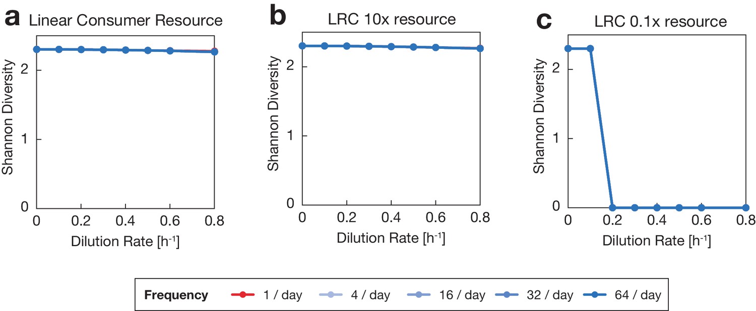
Linear Consumer Resource models do not exhibit relationship between diversity and fluctuation.
Shannon diversity was plotted vs. disturbance intensity (mean dilution rate), taking the mean across 100 communities after 6 days of simulated growth. Fluctuations are classified by frequency of dilution disturbance, indicated by color. (a) Shannon diversity for linear consumer resource (LRC) model shows no relationship between diversity and fluctuations. (b) Simulations were run with increased resource supply concentrations (), which did not affect the DDR. (c) Simulations were run with decreased resource supply concentrations (). This reduced growth rates to a level below the dilution rate, leading to washout and a corresponding Shannon diversity of zero.
Appendix 1—figure 3
Comparison between Monod consumer resource models with variant parameter choices reveal those that retain U-shape.
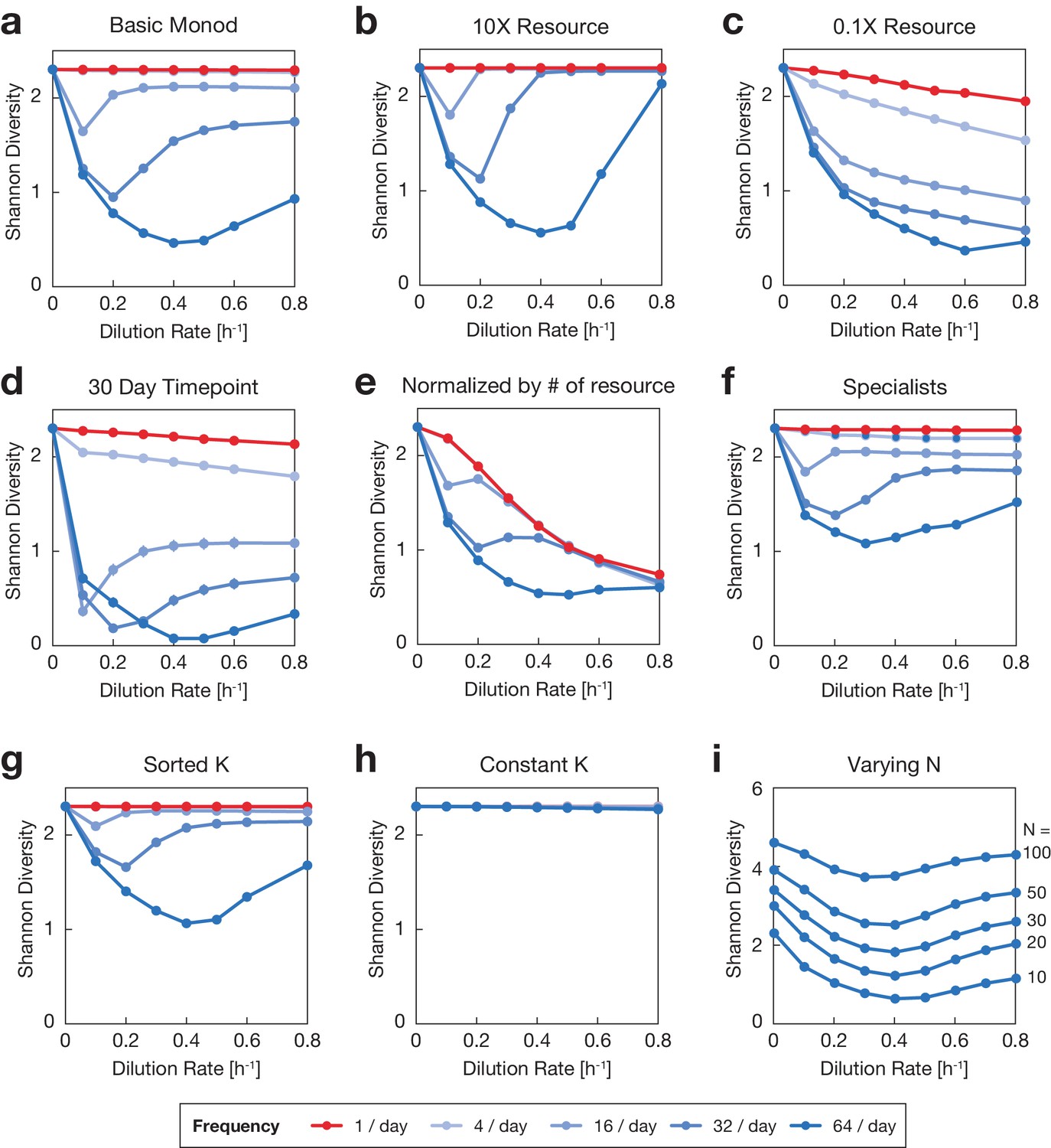
Each plot displays Shannon diversity after 6 days of simulated growth, mean across 100 communities for varying mean dilution rate and dilution frequency (see legend). Variations on the basic Monod model are discussed in Materials and methods. (a) Basic Monod Growth model, reproduced from Figure 3e. (b) Increasing resource supply by a factor of 10 does not qualitatively change the DDR. (c) Decreasing resource supply by a factor of 10 strongly affects the DDR by moving the competition out of the saturating nutrient range (set by ), such that the Monod model approaches a linear consumer resource model. (d) Carrying out the basic Monod growth model from a over longer simulation lengths retains the qualitative DDR shape. (e) Randomized growth rates on each resource were normalized by the number of resources rather than the species summed growth rates, which permitted wide variance in overall species growth rates, but retained some U-shape. (f) Simulations of communities of 10 species of specialists that consumed only 3 out of 7 resources exhibited higher diversity, but retained U-shaped DDRs. (g) Sorted simulations, reproduced from Appendix 2—figure 1. (h) Constant simulations, in which a randomly selected is shared for all species and resources, do not show U-shape. (i) Simulations of communities with varying N number of species and equal number of N resources exhibit U-shaped DDRs under 64/day dilution frequencies.
Appendix 1—figure 4

Comparison between Monod consumer resource models with variant assumptions can retain U-shape.
Each plot displays Shannon diversity after 6 days of simulated growth, mean across 100 communities for varying mean dilution rate and dilution frequency (see legend). Variations on the basic Monod model are discussed in Materials and methods. (a) Growth rates across multiple resources were normalized using an alternative mixed-substrate utilization model, retaining the DDR shapes. (b) Rather than having equal mortality rates across species, each species was assigned an independent mortality rate in addition to the universal dilution rate . Diversity is reduced as species with higher mortality rates are penalized, but this does not qualitatively change the DDRs observed. (c) To account for migration, each species was assigned a migration rate from a universal source community, independent of the dilution rate. Though species are constantly reintroduced into the community, if the migration rates are low compared to growth and dilution rates, then there are no major qualitative changes to the observed DDRs.
Appendix 2—figure 1
Generating species with sorted and parameters prevents intersection of growth curves but not niche flip.
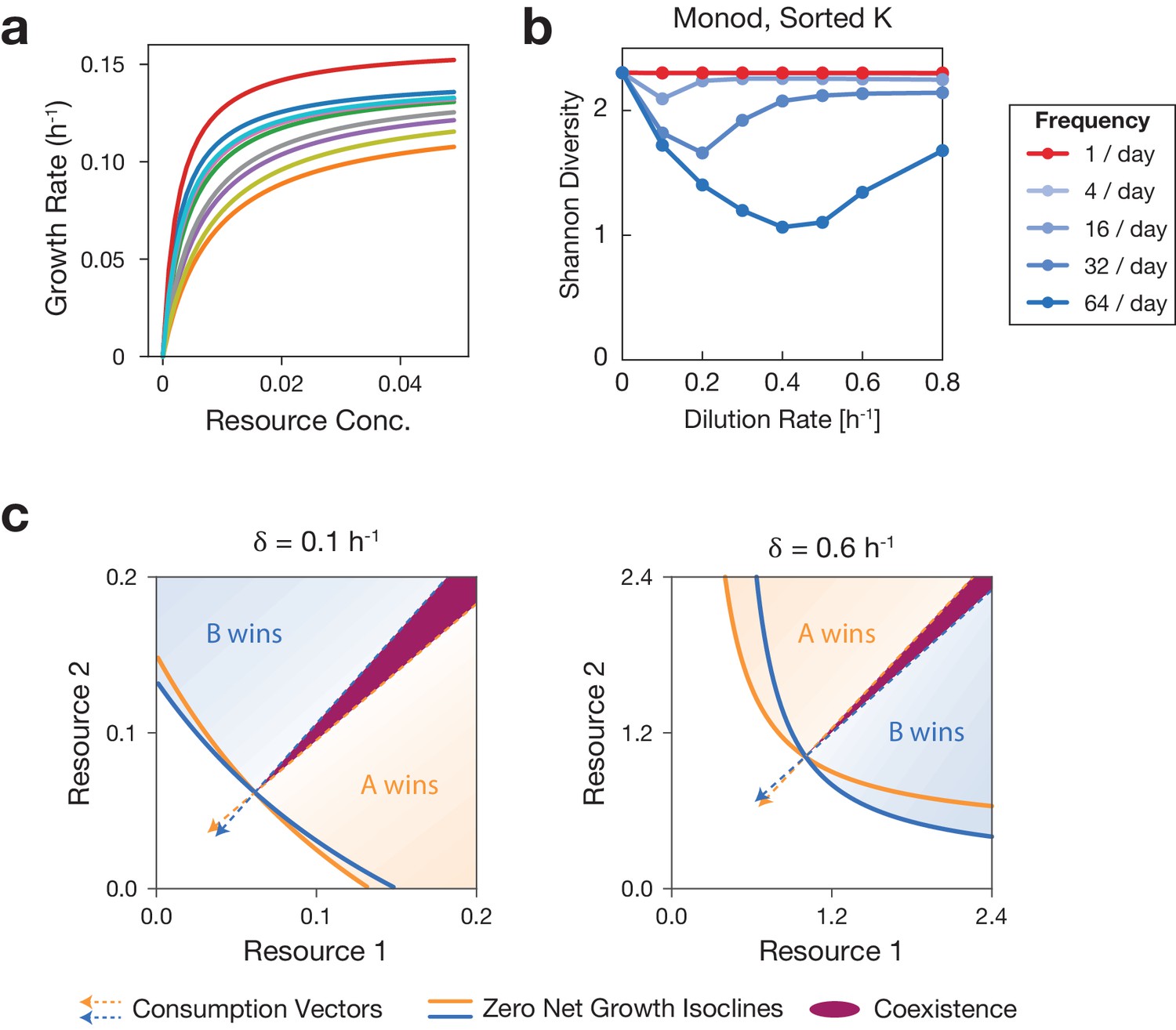
(a) Growth curves of 10 species on a single resource are shown. For these species in a single resource environment, the outcome of competition does not depend on resource concentration or dilution rate. (b) Communities with sorted per resource still exhibit U-shaped DDR. Shannon diversity of communities vs. mean dilution rate. Color indicates frequency of fluctuations. Calculations performed after 6 days of simulated growth, and averaged across 100 communities with randomly generated and sorted / parameters. (c) Niche flip occurs in a community with sorted parameters at high dilution rate. At low dilution rate, ZNGIs intersect the axes and the resource consumption vectors outline a coexistence region. At high dilution rate, species cannot survive on a single resource, so ZNGIs do not intersect the axis. The relative positions of ZNGIs and consumption vectors (i.e. invasion boundaries) have flipped at high dilution rate, consistent with niche-flip.
Additional files
Download links
A two-part list of links to download the article, or parts of the article, in various formats.
Downloads (link to download the article as PDF)
Open citations (links to open the citations from this article in various online reference manager services)
Cite this article (links to download the citations from this article in formats compatible with various reference manager tools)
Environmental fluctuations reshape an unexpected diversity-disturbance relationship in a microbial community
eLife 10:e67175.
https://doi.org/10.7554/eLife.67175


