Population receptive fields in nonhuman primates from whole-brain fMRI and large-scale neurophysiology in visual cortex
- Netherlands Institute for Neuroscience, Royal Netherlands Academy of Arts and Sciences, Netherlands
- Psychiatry Department, Amsterdam UMC, Netherlands
- Laboratory for Neuro- and Psychophysiology, Department of Neurosciences, KU Leuven Medical School, Belgium
- Massachusetts General Hospital, Martinos Ctr. for Biomedical Imaging, United States
- Leuven Brain Institute, KU Leuven, Belgium
- Harvard Medical School, United States
- Department of Integrative Neurophysiology, Center for Neurogenomics and Cognitive Research, VU University, Netherlands
Figures
Figure 1 with 1 supplement
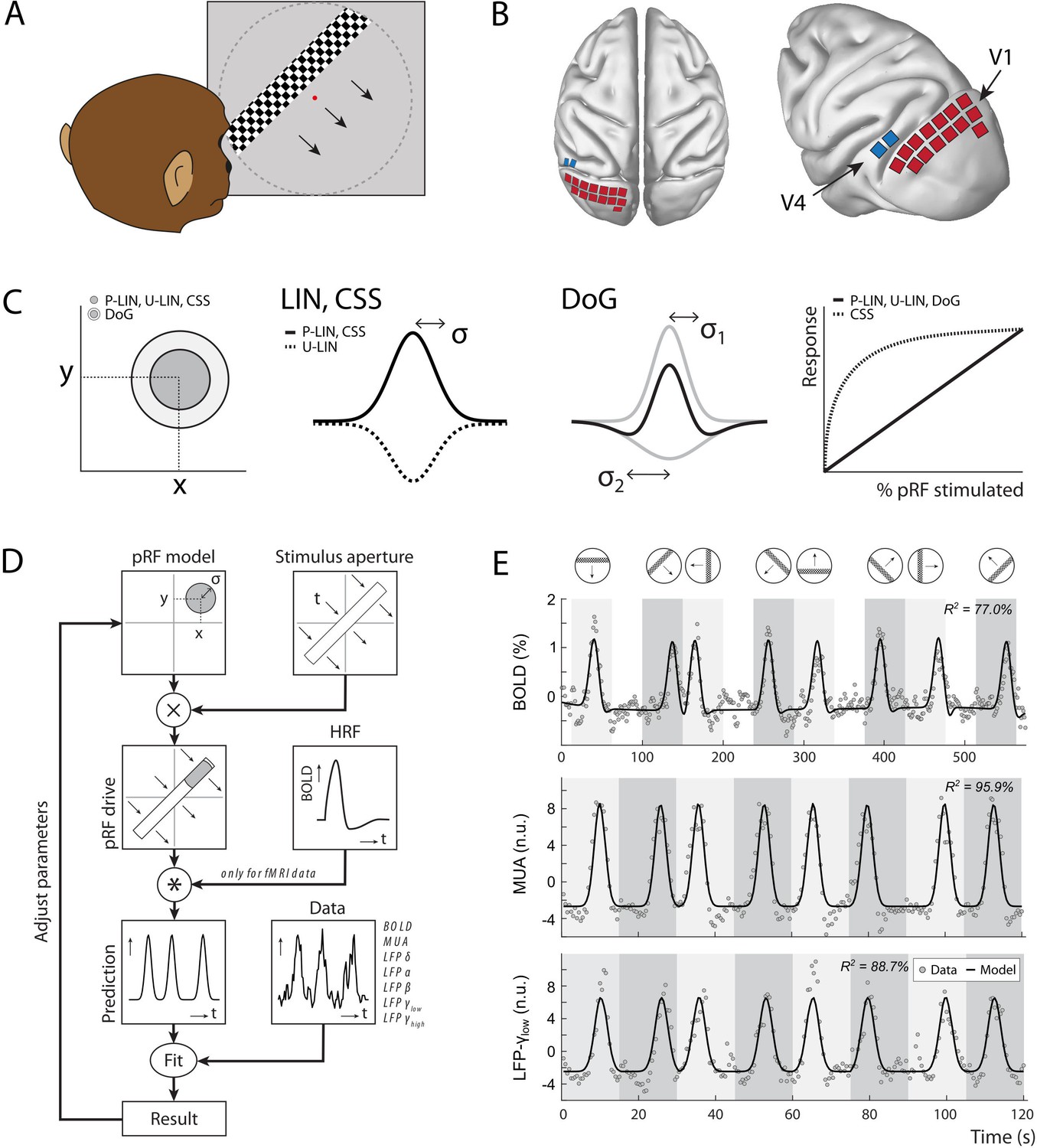
Experimental setup and study design.
(A) Monkeys maintained fixation on a red dot while bars with high-contrast-moving checkerboards moved across the screen in eight different directions behind a virtual aperture (dashed line, not visible in the real stimulus). (B) Two animals performed the task in the MRI scanner. Two other animals were each implanted with 16 Utah arrays (1024 electrodes/animal) in the left visual cortex. The approximate locations of 14 V1 arrays (red) and 2 V4 arrays (blue) for one animal are depicted on the NMT standard macaque brain. For more detailed array configurations, see Chen et al., 2020. (C) Four population receptive field (pRF) models were fit to the data, differing in their pRF parameters (location: x, y; size: σ) and spatial summation characteristics. The difference-of-Gaussians (DoG) pRFs are described by an excitatory center and an inhibitory surround (both 2D Gaussians with σ1 and σ2 as size parameters; dark and light gray circles in the left panel, respectively). Other models fitted single Gaussians that were either constrained to be positive (second panel: solid line) or allowed to be negative (unconstrained linear U-LIN, dashed line). The compressive spatial summation (CSS) model implemented nonlinear spatial summation across the receptive field (RF) (fourth panel: dashed line), while all other models implemented linear summation (solid line). (D) The pRF model fitting procedure. A model pRF is multiplied with an ‘aperture version’ of the bar stimulus to generate a predicted response. For fMRI data, this prediction was convolved with a monkey-specific hemodynamic response function (HRF). The difference between the recorded neural signal (blood-oxygen-level-dependent [BOLD], multi-unit activity [MUA], local field potential [LFP]) and the predicted response was minimized by adjusting the pRF model parameters. (E) Examples of data and model fits for a V1 voxel (top panel) and a V1 electrode (middle and bottom panels). Average activity (gray data points) depicts the BOLD signal (top), MUA (middle), and LFP power in the low gamma band (bottom). Black lines are the model fits for a P-LIN pRF model. Light and dark gray areas depict visual stimulation periods (bar sweeps as indicated by the icons above). In the white epochs, the animals viewed a uniform gray background to allow the BOLD signal to return to baseline (these epochs were not necessary in the electrophysiology recordings). Note that that in MRI trials the bar stimuli had a lower speed (1 TR or 2.5 s per stimulus location) than during electrophysiology (500 ms per stimulus location).
Figure 1—figure supplement 1
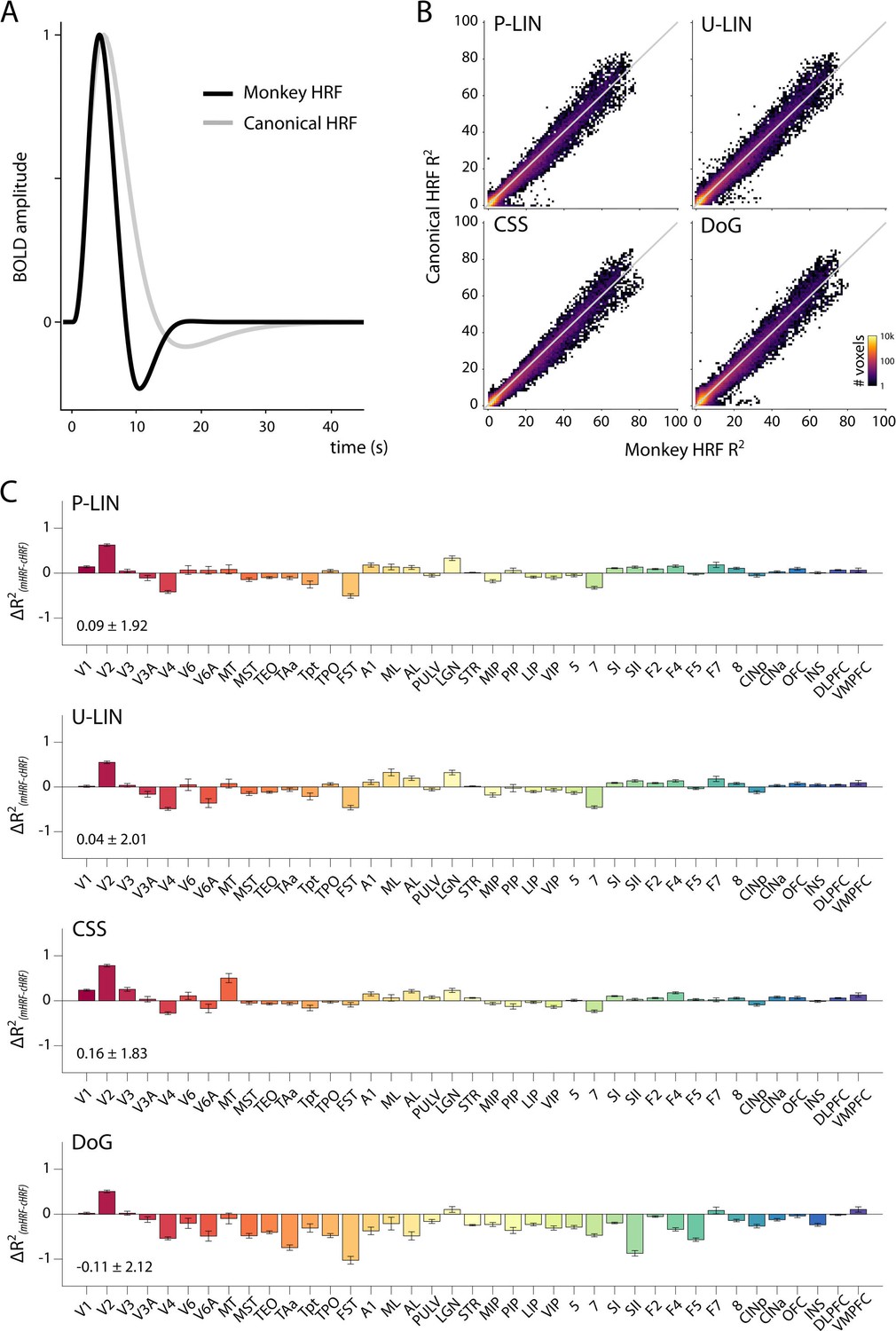
Comparison of hemodynamic response functions (HRFs).
(A) Population receptive field (pRF) models were fit to the blood-oxygen-level-dependent (BOLD) response with a monkey-specific (see Materials and methods) and a canonical HRF provided by the analyzePRF toolbox. The monkey HRF (black line) had a faster decay and more pronounced negative component than the canonical HRF (gray line). (B) The choice of HRF had a relatively small effect on the R2 of the models. The color map in this binned scatterplot (1 × 1% bins) indicates the number of voxels. For the P-LIN and compressive spatial summation (CSS) models, there was a small but significant advantage of using the specific monkey HRF over a canonical HRF in terms of the percentage of variance explained (Wilcoxon signed-rank, P-LIN: z = 8.41, p<0.0001; CSS: z = 16.39, p<0.0001). For the difference-of-Gaussians (DoG) model, the canonical HRF fits were consistently better in all areas except for the early visual areas, resulting in a significant advantage across all voxels overall (z = –29.79, p<0.0001). For the U-LIN model, the difference between HRFs was not significant for the analysis across all voxels (z = 0.97, p=0.33). In all cases, however, the effect sizes were very small (mean(mHRF-dHRF) ± standard deviation, P-LIN: 0.09% ± 1.92%; U-LIN: 0.04% ± 2.01%; CSS: 0.16% ± 1.83%; DoG: –0.11 ± 2.12%) and the estimated pRF sizes and locations were highly comparable across HRFs (Size(mHRF-dHRF), P-LIN: –0.07 ± 1.10 dva; U-LIN: –0.05 ± 1.68 dva; CSS: –0.19 ± 7.66 dva; DoG: –0.19 ± 1.68 dva; Eccentricity(mHRF-dHRF), P-LIN: –0.07 ± 2.13 dva; U-LIN: –0.09 ± 2.30 dva; CSS: –0.02 ± 1.93 dva; DoG: –0.08 ± 2.43 dva). For this reason, we only included the results obtained with the faster monkey-specific HRF in post-fit analyses of the MRI results. (C) Mean difference in R2 value between the HRFs for all models and regions of interest (ROIs). The monkey HRF produced slightly better fits in early visual areas for all models. For the DoG model, the canonical HRF fit slightly better in higher cortical areas. Number in lower-left corner is the mean R2 difference (HRFmonkey - HRFcanonical) ± standard deviation.
Figure 2 with 1 supplement
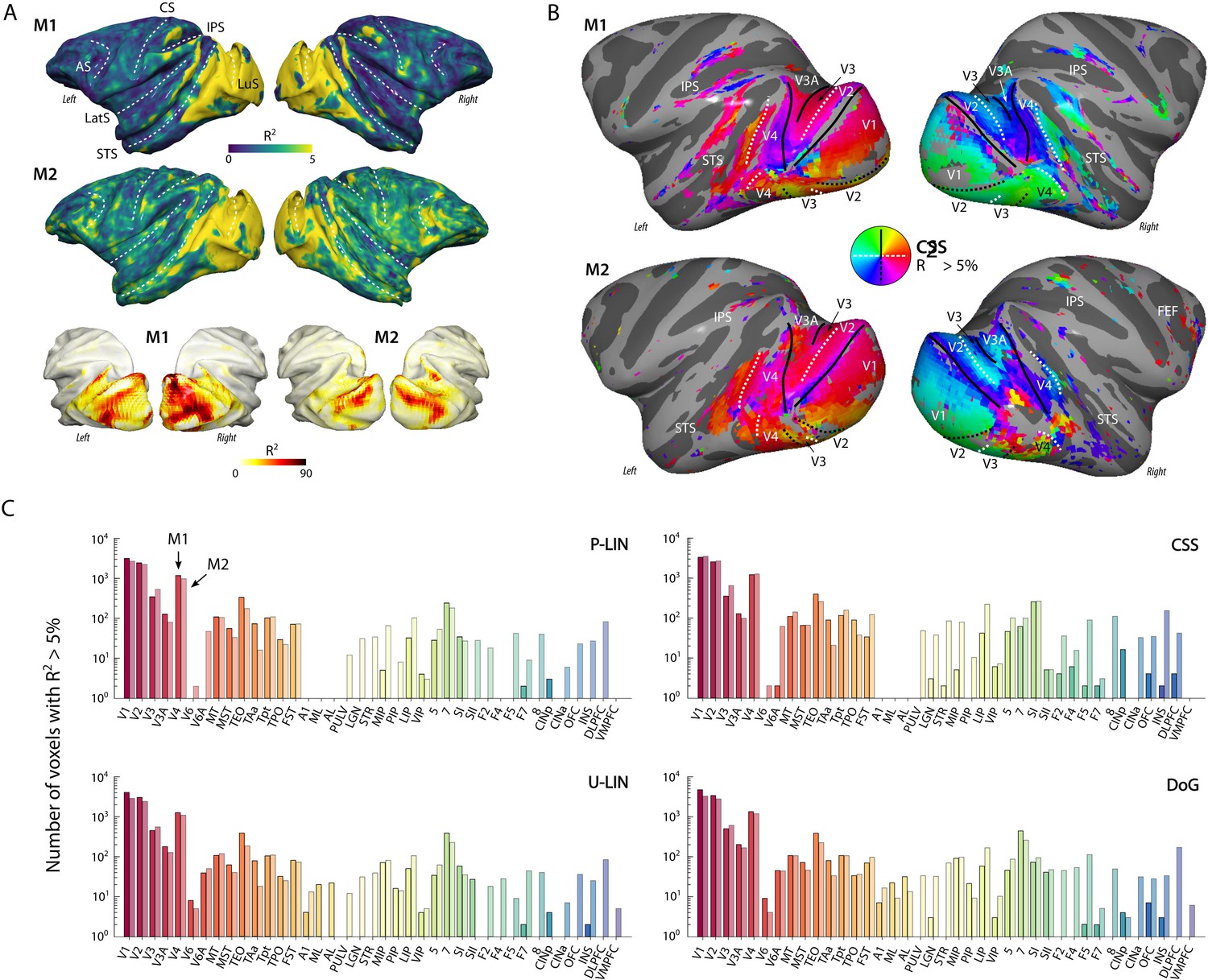
Population receptive field (pRF) model fits and retinotopic maps.
(A) R2 value map of the compressive spatial summation (CSS) pRF model projected on the surface rendering of the brains of two monkeys (M1, M2). The lower panel illustrates that the R2 value in the visual cortex is generally much higher than 5% (going up to ~90%). The color range in the upper panels also reveals the weaker retinotopic information elsewhere in the cortex. AS, arcuate sulcus; CS, central sulcus; IPS, intraparietal sulcus; LatS, lateral sulcus; LuS, lunate sulcus; STS, superior temporal sulcus. (B) Polar angle maps for both subjects from the CSS model, thresholded at R2 > 5%, displayed on the inflated cortical surfaces. Functional delineation of several visual areas is superimposed. FEF, frontal eye fields. (C) Number of (resampled) voxels with R2 > 5% per brain area and subject for each model. Note the logarithmic scale. See Figure 2—figure supplement 1 for proportions per region of interest (ROI), and Supplementary file 1 for a table with all ROI abbreviations.
Figure 2—figure supplement 1
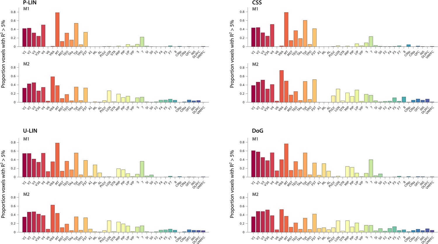
Proportion of voxels with R2 > 5% per region of interest (ROI).
For both animals (M1, M2) and all four population receptive field (pRF) models. This is supplement to Figure 2C that reports absolute numbers of voxels per area.
Figure 3 with 1 supplement
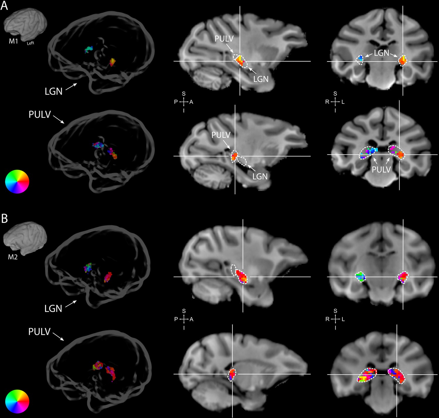
Retinotopy in the thalamus.
Thalamic population receptive fields (pRFs) in M1 (A) and M2 (B). The lateral geniculate nucleus (LGN, top rows) contained retinotopic maps of the contralateral visual field in both monkeys (M1: 38/38; M2: 73/80 voxels with contralateral pRFs). Retinotopic information was also present in the pulvinar (PULV, bottom rows), but its organization was much less structured, especially in M2 (M1: 23/32; M2: 61/131 voxels with contralateral pRFs). Voxels were thresholded at R2 > 3% for these polar angle visualizations due to the generally poorer fits in subcortex compared to visual cortex. Results from the compressive spatial summation (CSS) model are masked by region of interest (ROI) and shown both in a ‘glass’ representation of the individual animals’ brains (left), and on selected sagittal and coronal slices (monkey-specific T1-weighted images, cross-hairs indicate slice positions). Dashed lines indicate the boundaries of the LGN and pulvinar.
Figure 3—figure supplement 1
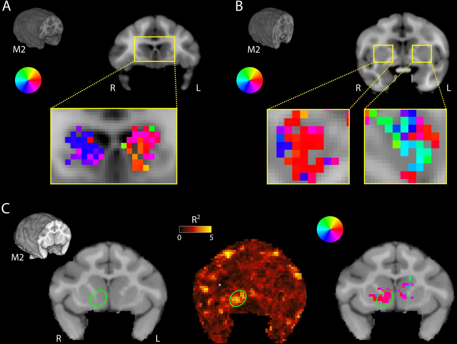
Striatal population receptive fields (pRFs).
(A) In M2, the head of the caudate nucleus in the striatum contained retinotopic maps of the lower contralateral visual field. Neurons in the head of the caudate have long been known to play a role in processing visual information in a reward-related context (Hikosaka et al., 1989a; Hikosaka et al., 1989b; Rolls et al., 1983). (B) In the more posterior striatum of M2, retinotopic information was also present. While spatial preferences were more mixed here, there was a dominant representation of the ipsilateral visual field. (C) Voxels in the right nucleus accumbens (NAc) have ipsilateral pRFs. The right NAc in the ventral striatum (green outline) is retinotopically tuned in both monkeys (only M2 shown). Although R2 values are lower than in the cortex or thalamus, they stand out from the surrounding regions. Polar angle maps of the fitted pRFs indicate that the right NAc is tuned to visual information in the right (ipsilateral) visual field.
Figure 4 with 2 supplements

Comparison of the four population receptive field (pRF) models.
(A) Comparison across pRF models. R2 data are in bins of 1% × 1%, and color indicates the number of voxels per bin. The compressive spatial summation (CSS) model fits the data best, while U-LIN and difference-of-Gaussians (DoG) models give better fits for voxels that are poorly characterized by the P-LIN model (arrows). Dashed triangle, voxels for which R2 of the U-LIN/DoG models was at least 5% higher than that of the P-LIN model. (B) Gain values of the U-LIN pRF fits for all voxels (black) and the voxels in the gray triangle in (A.) The negative gain values indicate visual suppression of the blood-oxygen-level-dependent (BOLD) signal. Arrows, medians. (C) Clusters of voxels for which the U-LIN model fit better than the P-LIN model were located in the medial occipital lobe (left panel). The pRFs of these voxels had a high eccentricity according to the P-LIN model, beyond the stimulated visual field. (D) Clusters of voxels with negative pRFs in the U-LIN model (without positive pRFs in the P-LIN model) were present around the lateral sulcus (LatS), in the medial occipital parietal cortex (mOP) and in the lateral occipital parietal cortex (lOP).
Figure 4—figure supplement 1

Comparison of fit performance across pRF models.
(A, B) Fit accuracy advantage of compressive spatial summation (CSS) and difference-of-Gaussians (DoG) models across brain areas. Both the CSS (A) and DoG (B) models had better fits (cross-validated R2) than the P-LIN model across virtually all brain regions with retinotopic information in both monkeys. (C) Comparison of R2 across population receptive field (pRF) models for both monkeys. Data are in R2 bins of 1% × 1%. Colors represent number of voxels per bin. The CSS model fits best across the board. The U-LIN and DoG models give good fits for voxels that are poorly characterized by the P-LIN model (arrows). Voxels for which the cross-validated R2 of the U-LIN or DoG models was >5% and at least 5% higher than that of the P-LIN or CSS are indicated by the dashed triangle.
Figure 4—figure supplement 2
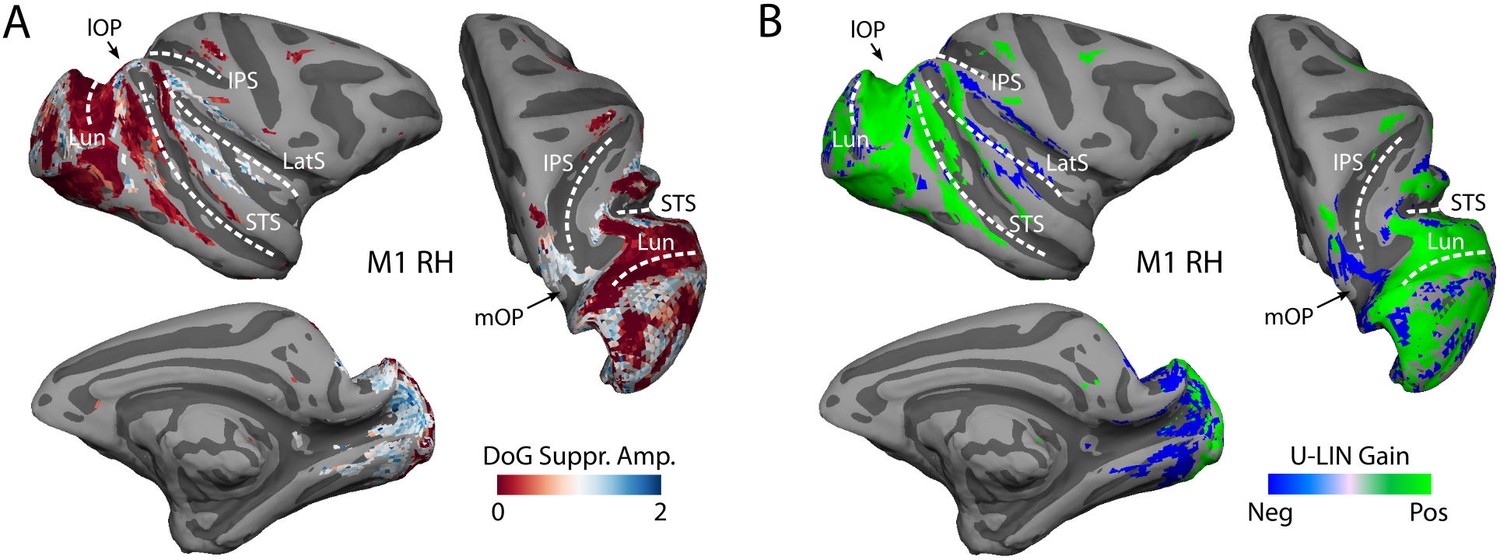
Location of negative pRFs.
(A) Normalized amplitude of the suppressive surround Gaussian of difference-of-Gaussians (DoG) model fits (R2 > 5%). Values larger than 1 (blue tints) indicate that the amplitude of suppressive surround was larger than that of the excitatory center. The right hemisphere of M1 is shown as an example. Voxels with a strong suppressive component were in the medial occipital and parietal cortices, and around the lateral sulcus. (B) Gain value of the of U-LIN fits for voxels with R2 > 5%. Green tints represent positive gain values, blue tints indicate suppressive blood-oxygen-level-dependent (BOLD) responses. Negative gain values occur for the same voxels that have a strong suppressive surround in (A), indicating that the activity of these voxels is suppressed by visual stimuli.
Figure 5 with 2 supplements
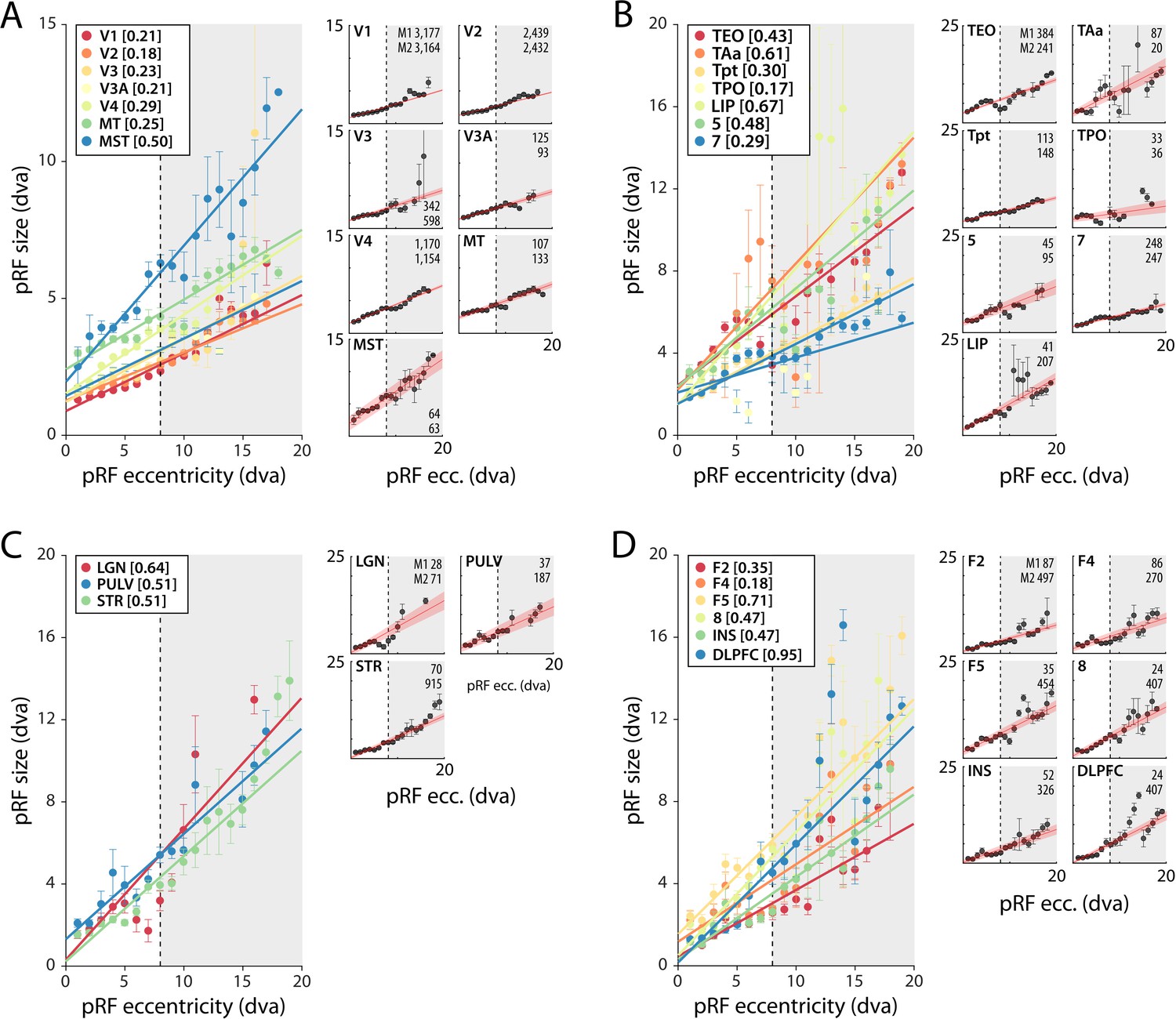
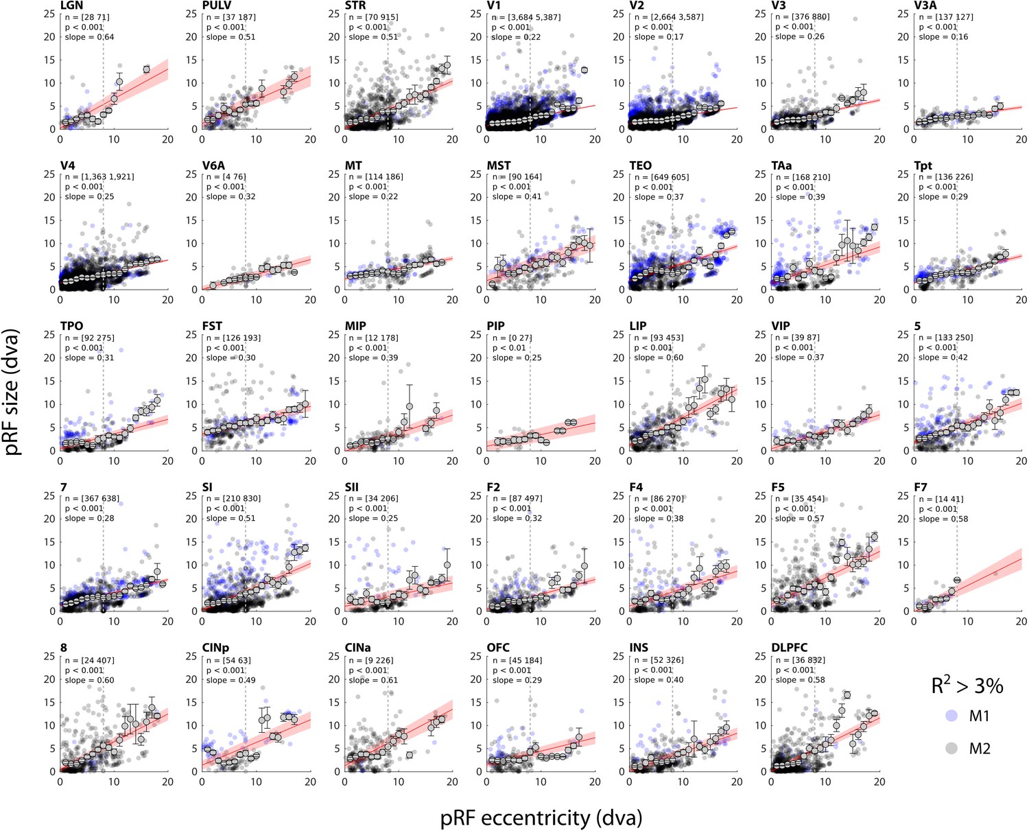
Population receptive field (pRF) size as a function of eccentricity according to the compressive spatial summation (CSS) model.
(A) Eccentricity-size relationship for early and mid-level visual areas. (B) Eccentricity-size relationship for areas in the temporal and parietal lobes. (C) Eccentricity-size relationship for subcortical areas. (D) Eccentricity-size relationship for frontal cortical areas. Data points are pRF sizes binned in 2-dva-eccentricity bins; error bars denote SEM. Lines are linear fits with a significant slope (p<0.01). Slope values are shown between square brackets in the legend. The dashed line that separates the white and gray areas indicates the extent of the visual stimulus used to estimate pRFs. Data points in the gray regions come for pRFs that fell partially outside the region with a visual stimulus. The small panels show the same data for individual areas and include confidence intervals of the linear fit (shaded red area). Numbers denote the number of voxels per animal. The displayed areas were selected based on the presence of at least 20 voxels in each animal, with R2 > 5% for (A, B) and R2 > 3% for (C, D) due to the generally lower fit quality in the subcortex and frontal lobe. Figure 5—figure supplements 1 and 2 plot all suprathreshold voxels.
Figure 5—figure supplement 1

Eccentricity-size relationship for all regions of interest (ROIs).
Linear fits (intercept and slope) to the eccentricity-size relationship per brain area. Shaded areas indicate the 95% confidence interval of the fit, n denotes the number of voxels (R2 > 5%). Linear fits in red have a significant slope (p<0.05). Small data points indicate population receptive fields (pRFs) for individual voxels (M1 in blue, M2 in black) while larger data points with error bars indicate binned averages (2 dva bins) over all voxels. The dotted vertical line indicates the extent of the visual stimulus.
Figure 5—figure supplement 2
Eccentricity-size relationship for all regions of interest (ROIs).
Linear fits (intercept and slope) to the eccentricity-size relationship per brain area. Shaded areas indicate the 95% confidence interval of the fit, n denotes the number of voxels (R2 > 3%). Linear fits in red have a significant slope (p<0.05). Small data points indicate population receptive fields (pRFs) for individual voxels (M1 in blue, M2 in black) while larger data points with error bars indicate binned averages (2 dva bins) over all voxels. The dotted vertical line indicates the extent of the visual stimulus.
Figure 6 with 1 supplement
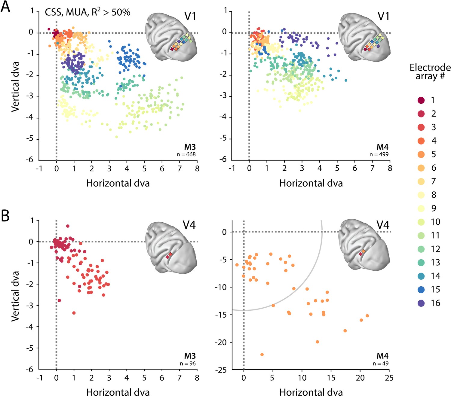
Visual field coverage of population receptive fields (pRFs) with Utah arrays.
(A) In both monkeys (M3, M4), 14 Utah arrays were implanted on the left operculum that is partly V1. Different colors represent the center of multi-unit activity (MUA)-based pRFs for the individual arrays. Only electrodes with R2 > 50% in the compressive spatial summation (CSS) model are shown. (B) Same as in (A), but for V4 electrodes. Note the different scale in the lower-right panel, with the gray arc indicating the extent of the visual stimulus. See Figure 6—figure supplement 1 for pRF sizes.
Figure 6—figure supplement 1
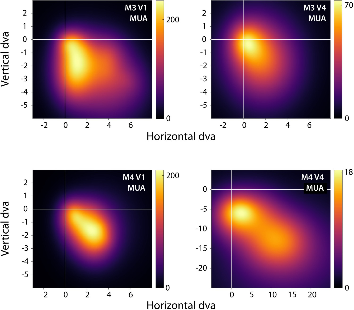
Heatmaps of visual field coverage of the Utah arrays.
We reconstructed the multi-unit activity (MUA) population receptive fields (pRFs) with R2 > 50% in the compressive spatial summation (CSS) model in the visual field, normalized them to their peak value, and then summed them across recording sites. The resulting heatmap represents the visual field coverage of V1 and V4 recording sites. The color scale represents the number of pRFs. See Figure 6 for individual pRF locations.
Figure 7
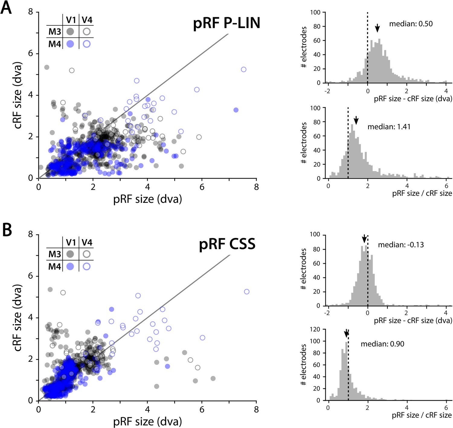
Comparison of multi-unit activity (MUA) population receptive field (pRF) sizes with conventionally determined RF (cRF) sizes (moving bar stimulus).
Data points represent recording sites of individual animals (black: M3; blue: M4) and brain areas (closed circles: V1; open circles: V4). (A) pRF sizes estimated with the P-LIN model (X-axis in left panel) are larger than cRF sizes obtained with a thin moving luminance bar (Y-axis in left panel). The median difference between pRF and cRF sizes across all electrodes (pooled across animals and areas) was 0.50 (interquartile range [IQR]: 0.08–0.92) and the median ratio was 1.41 (IQR: 0.99–1.83), as shown in the top and bottom-right panels, respectively. (B) As in (A), but for pRF sizes estimated with the compressive spatial summation (CSS) model, which are slightly smaller than the cRFs (median difference: –0.13, IQR: –0.41–0.14; median ratio 0.90, IQR: 0.67–1.12).
Figure 8 with 3 supplements
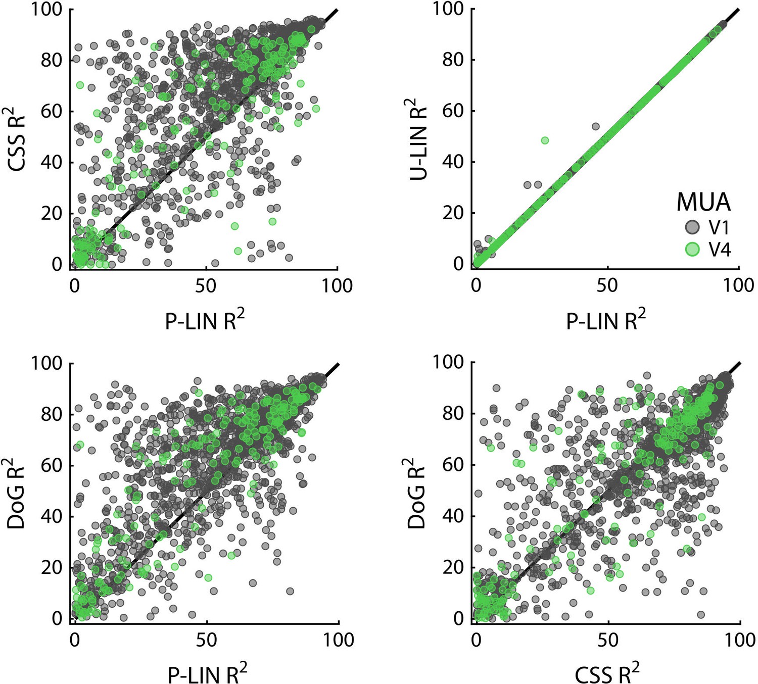
Comparison of multi-unit activity (MUA)-based fit results from the four population receptive field (pRF) models.
Scatterplots compare R2 of pRF models. Each dot represents an electrode (black: V1; green: V4).
Figure 8—figure supplement 1
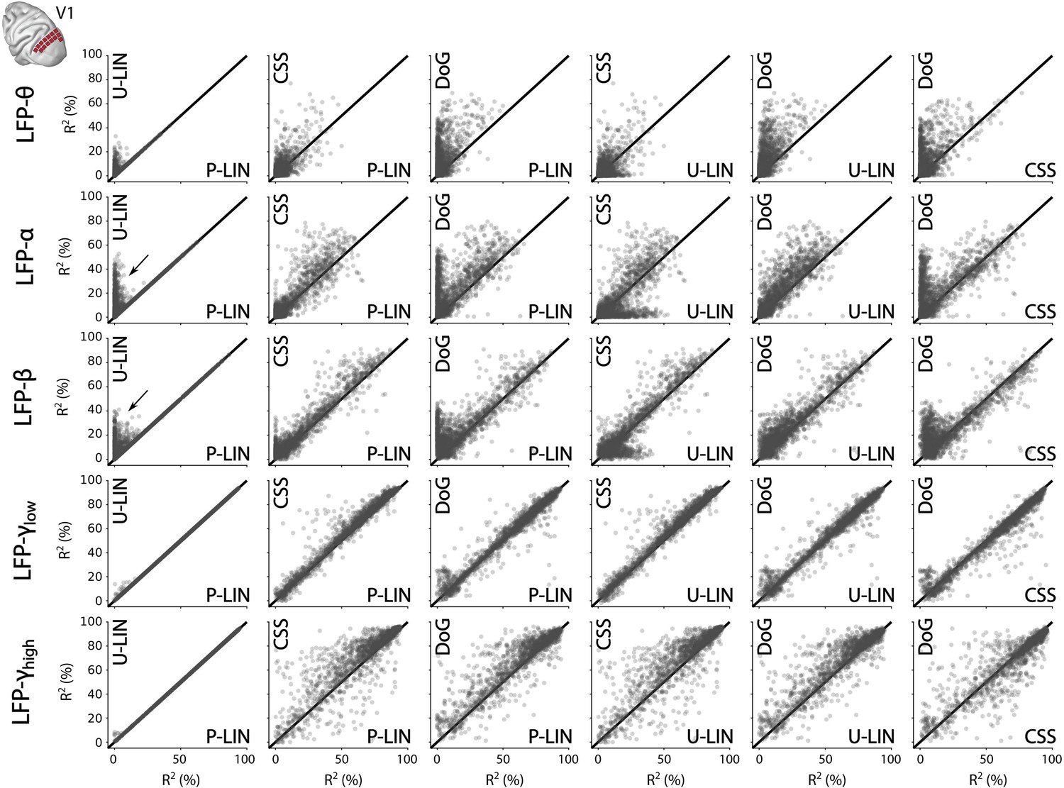
Comparison of local field potential (LFP) fits for the four population receptive field (pRF) models in V1.
Scatterplots compare R2 across pRF models and LFP frequency bands. Each dot represents an electrode. For a subset of electrodes, the pRF models that can capture negative responses (difference-of-Gaussians [DoG], U-LIN) fit better to the lower frequency components of the LFP (α, β) (e.g., arrows in leftmost column comparing P-LIN and U-LIN fits).
Figure 8—figure supplement 2
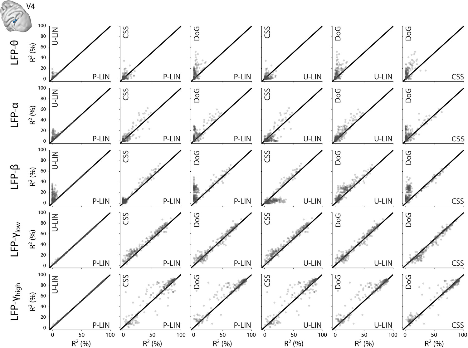
Comparison of local field potential (LFP)-based fit results from the four population receptive field (pRF) models in V4.
Scatterplots comparing R2 across pRF models and LFP frequency bands. Each data point represents an electrode.
Figure 8—figure supplement 3

Comparison of population receptive field (pRF) fit accuracies for multi-unit activity (MUA) and local field potential (LFP) signals at the same recording sites.
(A) Comparison of R2 values from the compressive spatial summation (CSS) model across electrophysiological signals. Colors indicate the number of recording sites in 4 × 4% bins (logarithmic scale). Asterisks denote significance (Kruskal–Wallis, with post-hoc Tukey’s HSD multiple comparisons of mean rank, *p<0.05, **p<0.001). (B–D) Same as in (A) but for the P-LIN (B), U-LIN (C), and difference-of-Gaussians (DoG) models (D).
Figure 9
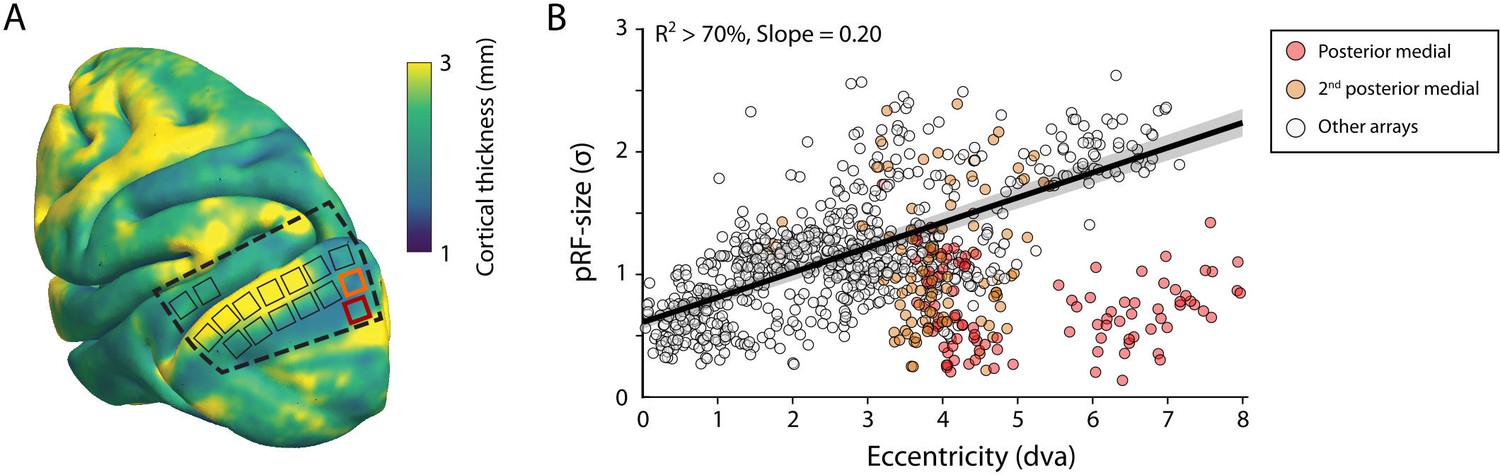
V1 arrays with outlying population receptive field (pRF) sizes.
(A) Schematic representation of the location of the craniotomy made during surgery (dashed line) and the implanted electrode arrays (rectangles) depicted on the NMT standard brain. The color map indicates the thickness of the cortical gray matter of the NMT. (B) For both monkeys, the estimated pRF sizes of V1 electrode arrays in the posterior medial corner of the craniotomy (red and orange data points correspond to red and orange rectangles in panel A) were surprisingly small for their eccentricity compared to the size-eccentricity relationship seen in the other arrays (gray circles, linear fit with 95% CI as black line and gray area). Given the length of the electrodes (1.5 mm), the typical thickness of the striate cortex, and these small pRF sizes, it is likely that the outlying pRFs do not reflect the tuning of V1 neurons, but that of the geniculostriate pathway in the white matter. The pRF sizes were estimated by the compressive spatial summation (CSS) model (recording sites shown have R2 > 70%).
Figure 10 with 2 supplements
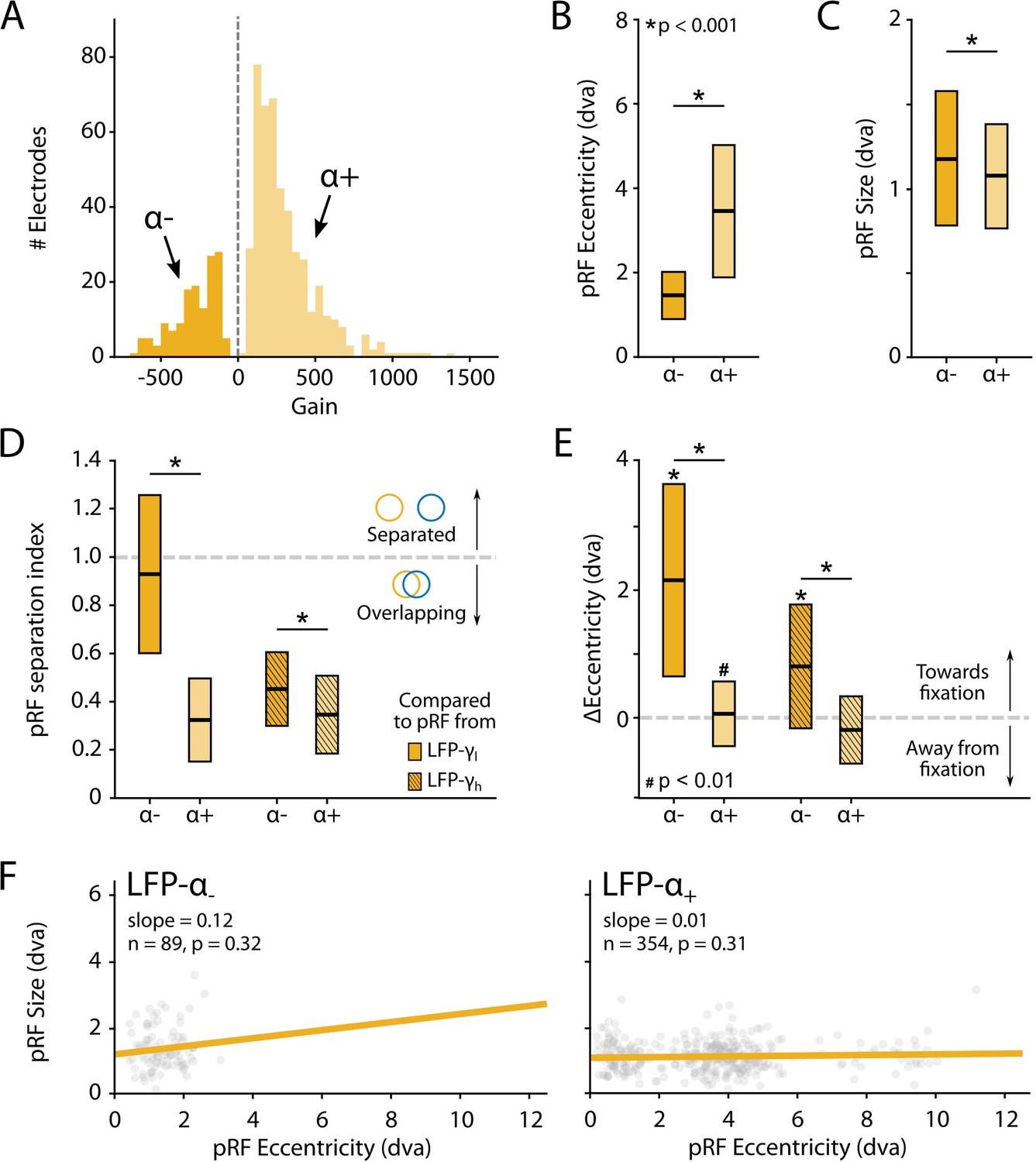
Characteristics of local field potential (LFP)-α population receptive fields (pRFs) in V1 split by positive and negative gain values.
(A) Distribution of gain values for LFP-α pRFs of V1 electrodes estimated with the U-LIN model. Electrodes with positive gain pRFs are classified as α+, electrodes with negative gain pRFs as α-. (B, C) pRF eccentricities (B) and size (C) for α- and α+ electrodes (yellow shades). Colored boxes indicate interquartile range (IQR), and the median is shown as a thick horizontal line. Wilcoxon rank-sum tests were used for comparisons between α- and α+ electrodes. (D) Distance between the centers of LFP-α and LFP-γ pRFs from the same electrode, divided by the sum of their respective sizes. Values smaller than 1 indicate overlapping receptive fields. Nonshaded boxes are comparisons with LFP-γlow pRFs, shaded boxes are comparisons with LFP-γhigh pRFs. (E) Difference in eccentricity between LFP-γ and LFP-α pRFs from the same electrodes (calculated as Eccγ-Eccα). Positive values indicate that LFP-α pRFs are closer to fixation than LFP-γ pRFs. Wilcoxon signed-rank, one-tailed test (ΔEcc > 0), for individual cases; Wilcoxon rank-sum test for comparisons between α- and α+ electrodes. See Figure 10—figure supplement 2 for a visualization of the shifts per recording site. (F) Eccentricity-size relationship for α- (left) and α+ (right) electrodes. Dots indicate individual electrodes. Figure 10—figure supplement 1 shows the same pattern of results for the LFP-β pRFs.
Figure 10—figure supplement 1
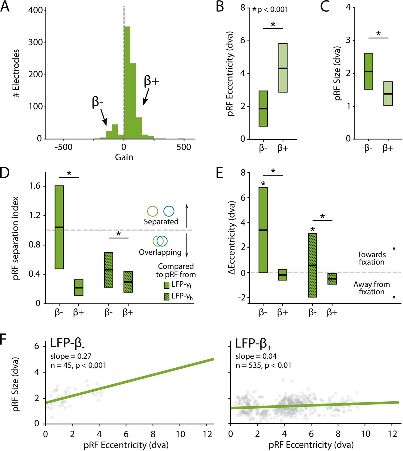
Characteristics of local field potential (LFP)-β population receptive fields (pRFs) in V1 split by positive and negative gain values.
(A) Distribution of gain values for LFP-β pRFs of V1 electrodes estimated with the U-LIN model. Recording sites with positive gain pRFs are classified as β+, sites with negative gain pRFs as β-. (B, C) pRF eccentricities (B) and size (C) for β- and β+ electrodes (yellow shades). Colored boxes indicate interquartile range (IQR), and the median is shown as a thick horizontal line. Wilcoxon rank-sum tests were used for comparisons between β- and β+ electrodes. (D) Distance between the centers of LFP-β and LFP-γ pRFs from the same electrode, divided by the sum of their respective sizes. Values smaller than 1 indicate overlapping receptive fields. Nonshaded boxes are comparisons with LFP-γlow pRFs, shaded boxes are comparisons with LFP-γhigh pRFs. (E) Difference in eccentricity between LFP-γ and LFP- β pRFs from the same sites (calculated as Eccγ-Eccα). Positive values indicate that LFP- β pRFs are closer to fixation than LFP-γ pRFs. Wilcoxon signed-rank, one-tailed test (ΔEcc > 0), for individual cases; Wilcoxon rank-sum test for comparisons between β- and β+ electrodes. See Figure 10—figure supplement 2 for a visualization of the shifts per recording site. (F) Eccentricity-size relationship for β- (left) and β+ (right) electrodes. Dots indicate individual electrodes.
Figure 10—figure supplement 2
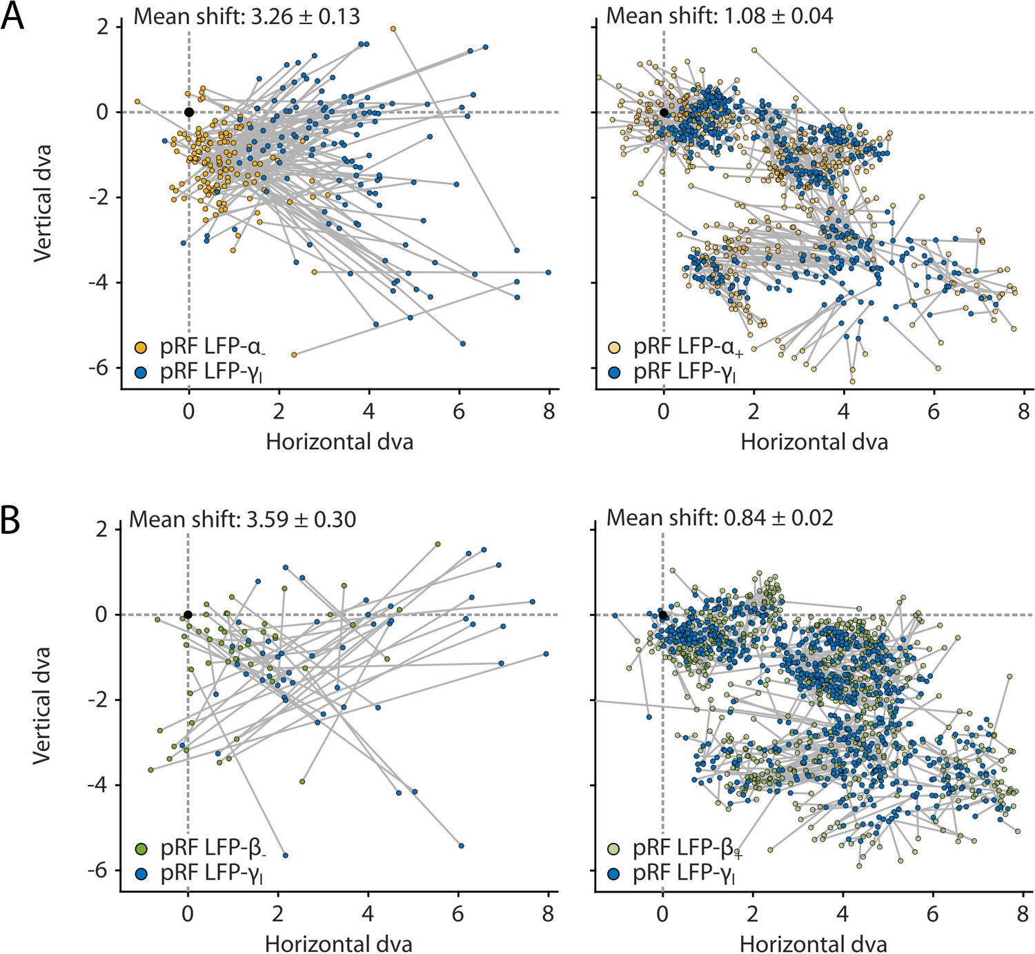
Negative population receptive fields (pRFs) based on low-frequency local field potential (LFP) components are shifted toward the fixation point compared to the positive pRFs based on the high-frequency LFP at the same recording site.
(A) Relative locations of pRFs derived from LFP-α (yellow) and LFP-γl (blue) of the same recording sites. (B) Relative locations of pRFs derived from LFP-β (green) and LFP-γl (blue) of the same recording sites. Data points from the same sites are connected with a gray line. The location of the fixation point is indicated with a black dot. The mean shift size ± SEM is listed in each panel. The same data were used to calculate the eccentricity shifts that are summarized in Figure 10E and Figure 10—figure supplement 1E.
Figure 11
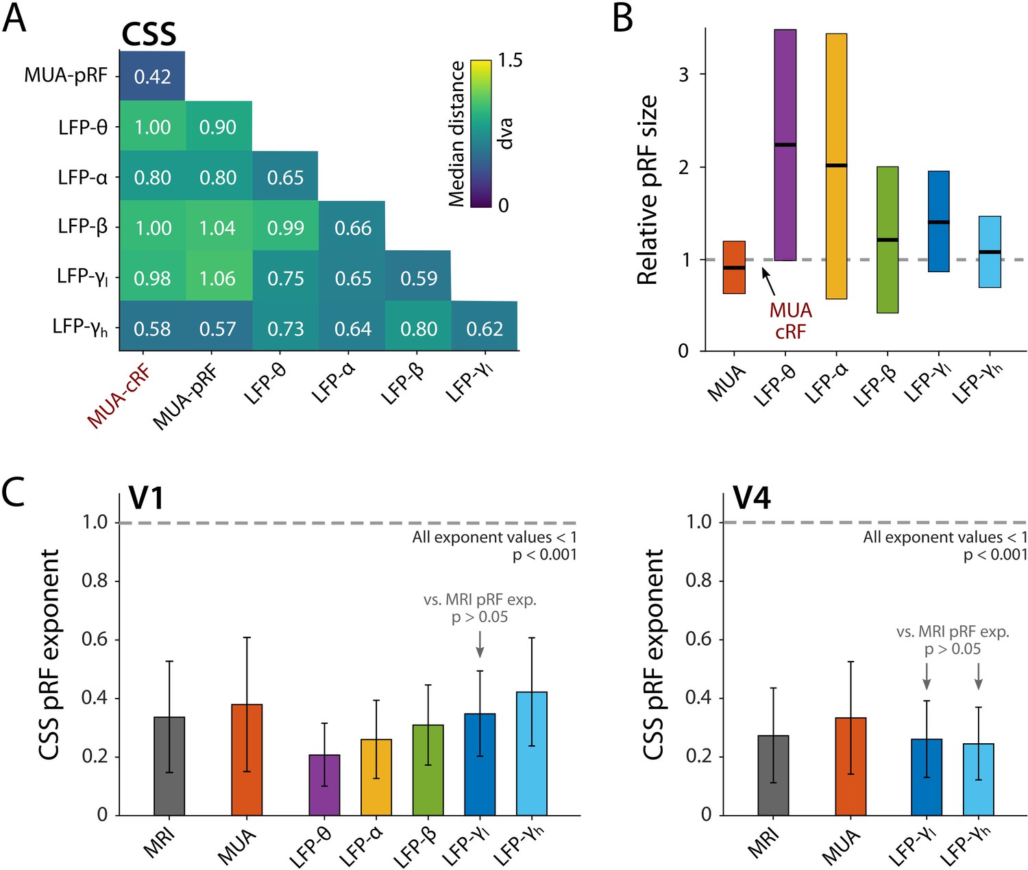
Comparison of population receptive field (pRF) location and size of different electrophysiological signals at the same electrode, estimated by the compressive spatial summation (CSS) model.
(A) Median distance between receptive field (RF) estimates. Electrodes were only included if R2 > 25% (multi-unit activity [MUA], local field potential [LFP]) or signal-to-noise ratio (SNR) > 3 (MUA-cRF). (B) RF size for the electrodes of (A), normalized to the MUA-cRF (dashed line). Horizontal lines indicate the median, colored rectangles depict the interquartile range (IQR). (C) pRF exponent from the CSS model (indicating nonlinearity of spatial summation). The horizontal dashed line indicates linear summation. The exponent was significantly lower than 1 for all signals. Gray arrows indicate signals for which the exponent did not significantly differ from that of the MRI pRFs. A similar pattern was present in the electrophysiological data of each animal.
Figure 12 with 1 supplement

Eccentricity-size relationship for population receptive fields (pRFs) across signal types.
(A) The pRF size-eccentricity relation for V1 electrodes (compressive spatial summation [CSS] model, R2 > 50%). Dots are individual electrodes, colored lines represent the slope of the eccentricity-size relationship. The dashed black line represents the relationship for V1 MRI voxels with a pRF in the lower-right visual quadrant and an R2 > 5%. We only included signals with >25 electrodes meeting the R2 threshold. (B) Same as in (A), but now for the V4 electrodes and voxels. (C) Eccentricity-size slopes (left: V1; right: V4). The dashed line represents the slope for MRI-based pRFs with the 95% confidence interval depicted in gray shading. Colored rectangles indicate the 95% confidence intervals for the electrophysiological signals and the horizontal black line the slope estimate. The lower bound of the 95% confidence interval of the LFP-θ is not visible. Asterisks indicate significant difference with the size-eccentricity relation of the MRI-based pRFs.
Figure 12—figure supplement 1
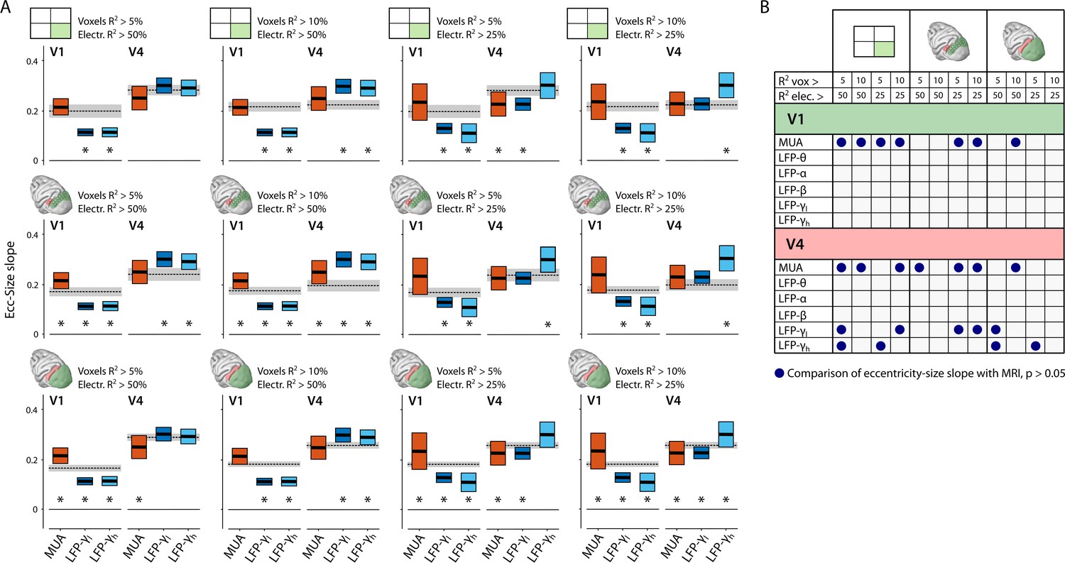
Cross-signal comparisons of population receptive field (pRF) eccentricity-size relationship.
(A) The results of the cross-signal comparisons of compressive spatial summation (CSS)-pRF-based eccentricity-size slopes for different data inclusion criteria. For the top row, we only included V1 and V4 voxels with pRFs in the lower-right visual field where we had electrode coverage. For the middle row, we only included voxels corresponding to the location of the electrode arrays. For the bottom row, we included all V1 and V4 voxels. Columns indicate different combinations of R2 threshold level for inclusion of selected voxels and electrodes. The black dashed line and gray area indicate the slope and 95% CI for the MRI-based pRFs; black horizontal lines and colored boxes denote the estimated slope for electrophysiology signals and their 95% CI. Asterisks indicate a significant difference of the eccentricity-size relation between MRI and electrophysiology. (B) Summary table of the results in (A), for all electrophysiology signals. Blue dots indicate the inclusion criterion for which the eccentricity-size slope of the pRFs from an electrophysiology signal was not significantly different from that of the MRI signal.
Tables
Key resources table
| Reagent type (species) or resource | Designation | Source or reference | Identifiers | Additional information |
|---|---|---|---|---|
| Biological sample(Macaca mulatta) | Rhesus macaque (Macaca mulatta), male | Biomedical Primate Research Center, the Netherlands | n/a | - |
| Other | Philips Ingenia 3.0T MR system | Philips | n/a | At Spinoza Centre for Neuroimaging, Amsterdam, the Netherlands |
| Other | 8-channel phased array receive MR coil system | KU Leuven | n/a | Custom-built |
| Other | 16-channel MR pre-amplifier | MR Coils BV | n/a | Custom-built |
| Other | ETL-200 | ISCAN | RRID:SCR_021044 | MR-compatible eye tracker |
| Other | E3X-NH | Omron | n/a | Fiber optic amplifiers |
| Other | 5-RLD-E1 Liquid Reward System | Crist Instrument Company, Inc | n/a | Juice reward system |
| Other | BOLDscreen 32 LCD for fMRI | Cambridge Research Systems | n/a | MR-compatible display |
| Other | Utah array (electrodes) | Blackrock Microsystems | n/a | - |
| Other | 128-channel CerePlex M head-stages | Blackrock Microsystems | n/a | Data acquisition |
| Other | 128-channel CerePlex M head-stages | Blackrock Microsystems | n/a | Data acquisition |
| Other | 128-channel Digital Hub | Blackrock Microsystems | n/a | Data acquisition |
| Other | 128-channel Neural Signal Processor (NSP) | Blackrock Microsystems | n/a | Data acquisition |
| Software, algorithm | Blackrock Central Software Suite | Blackrock Microsystems | n/a | - |
| Other | ET-49C | Tomas Recording | n/a | Eye tracker |
| Software, algorithm | MATLAB | MathWorks | RRID:SCR_001622 | - |
| Other | LISA cluster | SURFsara | n/a | Computing cluster |
| Software, algorithm | dcm2niix | https://github.com/rordenlab/dcm2niix | RRID:SCR_01409 | - |
| Software, algorithm | Nipype | http://nipy.org/nipype/ | RRID:SCR_002502 | Used as the basis of the custom NHP-BIDS pipeline |
| Software, algorithm | NHP-BIDS | Netherlands Institute for Neuroscience | RRID:SCR_021813 | In-house developed, available via: https://github.com/VisionandCognition/NHP-BIDS |
| Software, algorithm | FreeSurfer | http://surfer.nmr.mgh.harvard.edu/ | RRID:SCR_001847 | Used as the basis of the custom NHP-Freesurfer |
| Software, algorithm | NHP-Freesurfer | Netherlands Institute for Neuroscience | RRID:SCR_021814 | In-house developed, available via: https://github.com/VisionandCognition/NHP-Freesurfer |
| Software, algorithm | Pycortex | https://gallantlab.github.io/pycortex/ | n/a | Used as the basis of the customized NHP-Pycortex |
| Software, algorithm | NHP-Pycortex | Netherlands Institute for Neuroscience | RRID:SCR_021815 | In-house developed, available via: https://github.com/VisionandCognition/NHP-pycortex |
| Software, algorithm | analyzePRF | https://kendrickkay.net/analyzePRF/ | n/a | Toolbox was edited for this study and made available with the code and data |
| Software, algorithm | Jupyter Notebook | https://jupyter.org/ | RRID:SCR_018315 | - |
| Software, algorithm | FSL | http://www.fmrib.ox.ac.uk/fsl/ | RRID:SCR_002823 | - |
| Software, algorithm | Tracker-MRI: Experiment control software | Netherlands Institute for Neuroscience | RRID:SCR_021816 | In-house developed, available via: https://github.com/VisionandCognition/Tracker-MRI |
| Other | NMT v1.3 | NIH, AFNI https://afni.nimh.nih.gov/pub/dist/doc/htmldoc/nonhuman/macaque/template_nmtv1.html#nmt-v1-3 | n/a | Macaque Brain Template and Atlas |
Additional files
-
Supplementary file 1
Table with region of interest (ROI) abbreviations.
List of ROI abbreviations, color coded by where in the brain they are located.
- https://cdn.elifesciences.org/articles/67304/elife-67304-supp1-v3.docx
-
Transparent reporting form
- https://cdn.elifesciences.org/articles/67304/elife-67304-transrepform1-v3.pdf
Download links
A two-part list of links to download the article, or parts of the article, in various formats.
Downloads (link to download the article as PDF)
Open citations (links to open the citations from this article in various online reference manager services)
Cite this article (links to download the citations from this article in formats compatible with various reference manager tools)
Population receptive fields in nonhuman primates from whole-brain fMRI and large-scale neurophysiology in visual cortex
eLife 10:e67304.
https://doi.org/10.7554/eLife.67304


