Modeling spinal locomotor circuits for movements in developing zebrafish
- Brain and Mind Research Institute, Centre for Neural Dynamics, Department of Biology, University of Ottawa, Canada
- Blue Brain Project, École Polytechnique Fédérale de Lausanne, Switzerland
- Washington University School of Medicine, Department of Neuroscience, United States
Figures
Figure 1
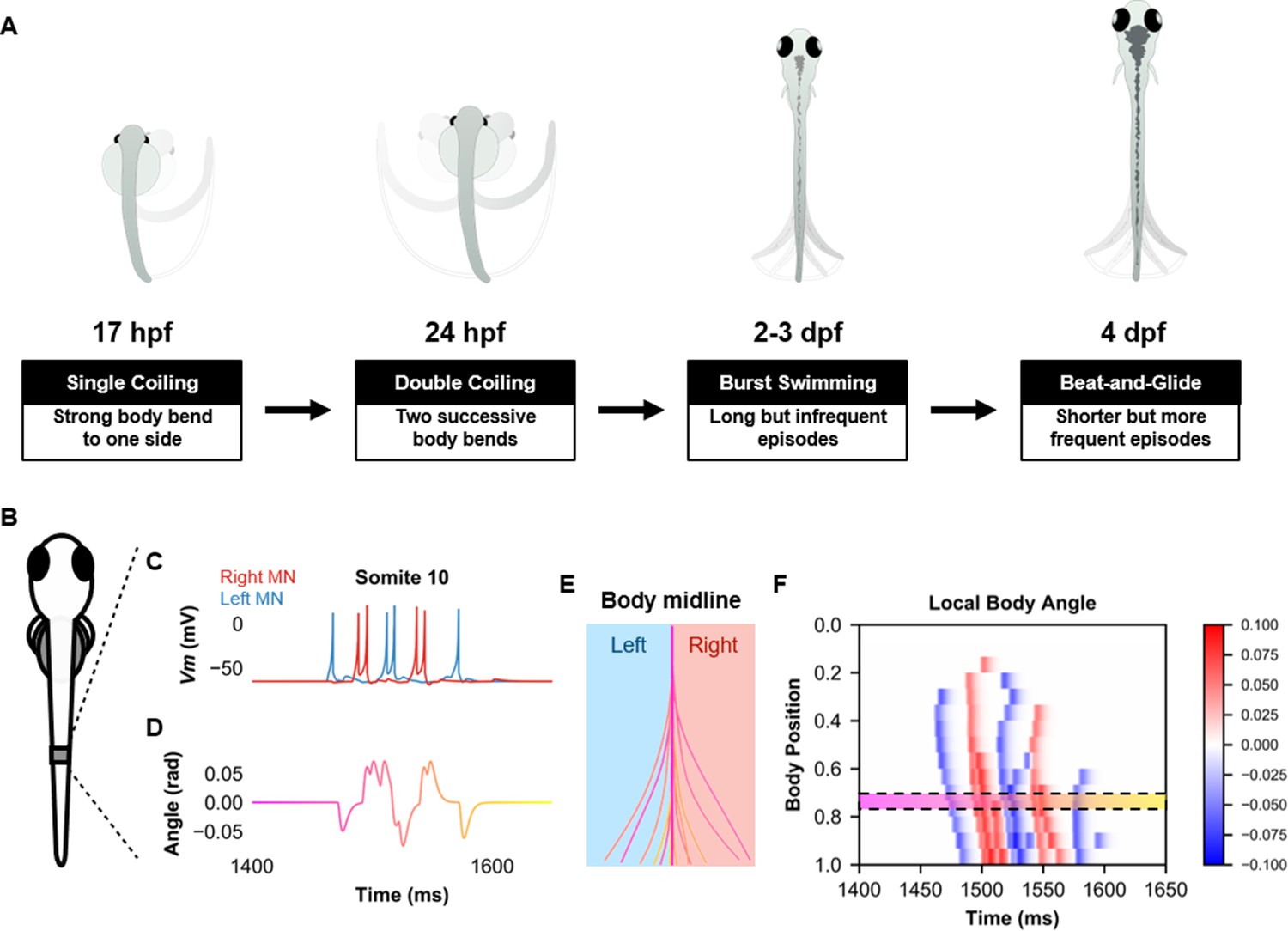
Simulation of the spinal locomotor circuit coupled to a musculoskeletal model during a beat-and-glide swimming episode.
(A) Schematic of locomotor movements during the development of zebrafish. (B) Schematic of a fish body with 10th somite outlined. (C) Motoneuron membrane potential (Vm) in the 10th somite during a single beat-and-glide swimming episode from our model is used to calculate this body segment’s body angle variation (D) in a musculoskeletal model. (E) Several representative body midlines from this episode of beat-and-glide swimming. Body midline is computed by compiling all the calculated local body angles along the simulated fish body. (F) Heat-map of local body angle (in radians) across the total body length and through time during the episode. Red is for right curvatures, while blue labels left curvatures. Body position on the ordinate, 0 is the rostral extremity, while 1 is the caudal extremity. In (D–F), the magenta to yellow color coding represents the progression through the swimming episode depicted.
Figure 2 with 4 supplements
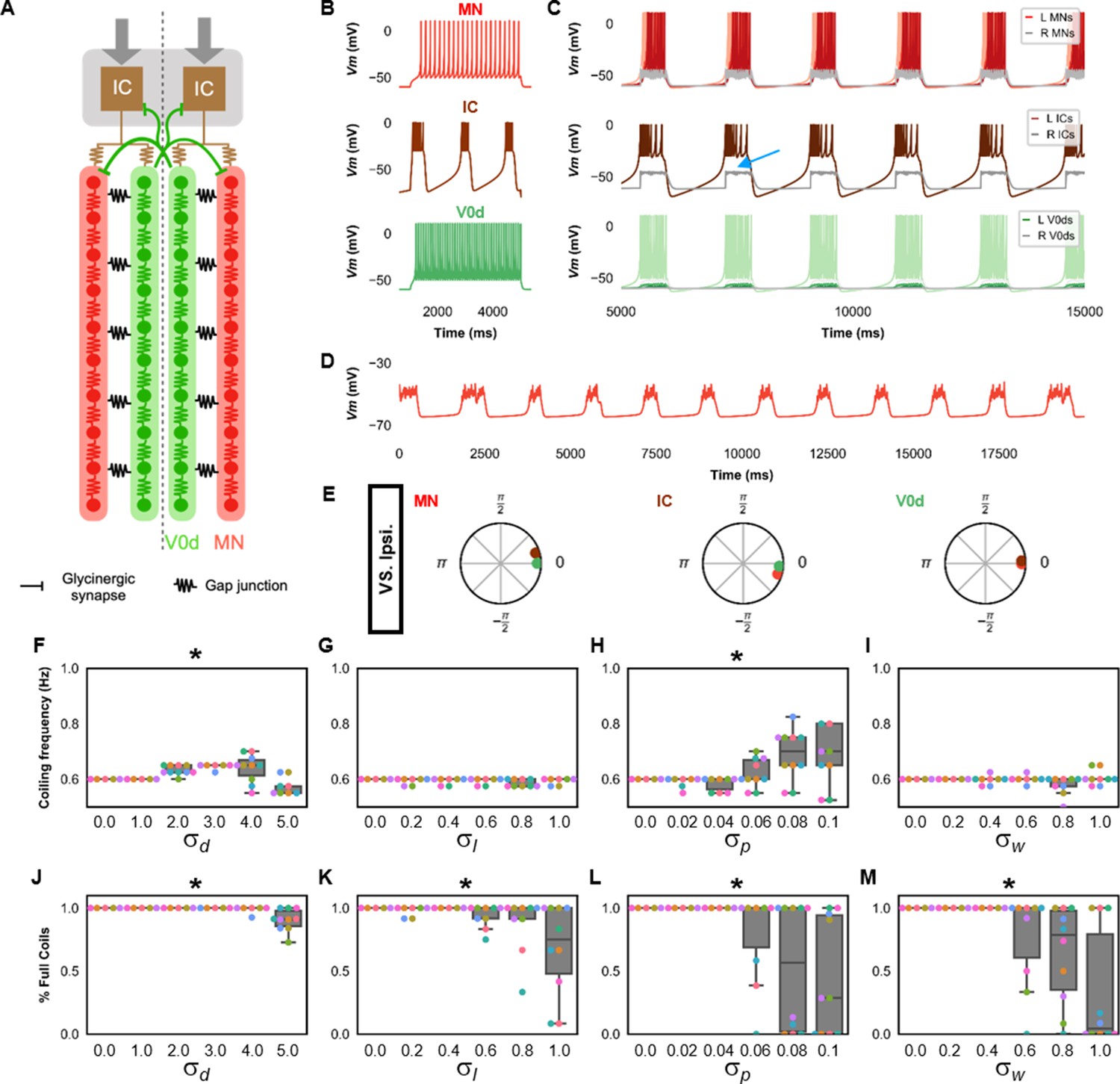
Single coiling model driven by pacemaker neurons.
(A) Schematic of the single coiling model. The dashed line indicates the body midline. Gray arrows indicate descending motor command. (B) Membrane potential (Vm) response of isolated spinal neuron models to a depolarizing current step. (C) Vm of spinal neurons during a simulation with a tonic command to left pacemakers only. Note the synaptic bursts in gray in the right MNs and IC neurons (a blue arrow marks an example). The Vm of a rostral (lightest), middle, and caudal (darkest) neuron is shown, except for IC neurons that are all in a rostral kernel. (D) Periodic depolarizations in a hyperpolarized motoneuron on the same side where single coils are generated. (E) The phase delay of left neurons in relation to ipsilateral spinal neurons in the first somite and an IC in the rostral kernel in a 10,000 ms simulation. The reference neuron for each polar plot is labeled, and all neurons follow the same color-coding as the rest of the figure. A negative phase delay indicates that the reference neuron precedes the neuron to which it is compared. A phase of 0 indicates that a pair of neurons is in-phase; a phase of π indicates that a pair of neurons is out-of-phase. Sensitivity testing showing (F–I) coiling frequency and (J–M) proportion of full coils during ten 20,000 ms simulation runs at each value of , , , and tested. Each run is color-coded. Bars on box plots represent 25th, median, and 75th percentile. Whiskers extend to 1.5 times the interquartile range. L: left, R: right. Statistics: Asterisks denote significant differences detected using a one-factor ANOVA test. (F) F5,59=10.4, p=5.2×10⁻⁷. (G) F5,59=2.4, p=0.05. (H) F5,59=5.2, p=0.0006. (I) F5,59=2.2, p=0.07. (J) F5,59=10.9, p=2.7×10⁻⁷. (K) F5,59=4.9, p=0.0009. (Note that there were no pairwise differences detected). (L) F5,59=6.5, p=8.2×10⁻⁵. (M) F5,59=8.8, p=3.5×10⁻⁶. P-values for t-tests are found in Figure 2—source data 1. See also Figure 2—figure supplements 1 and 2 and Figure 2—videos 1 and 2. IC, Ipsilateral Caudal; MN, motoneuron.
-
Figure 2—source data 1
P-values for sensitivity testing in single coiling model.
- https://cdn.elifesciences.org/articles/67453/elife-67453-fig2-data1-v2.xlsx
Figure 2—figure supplement 1
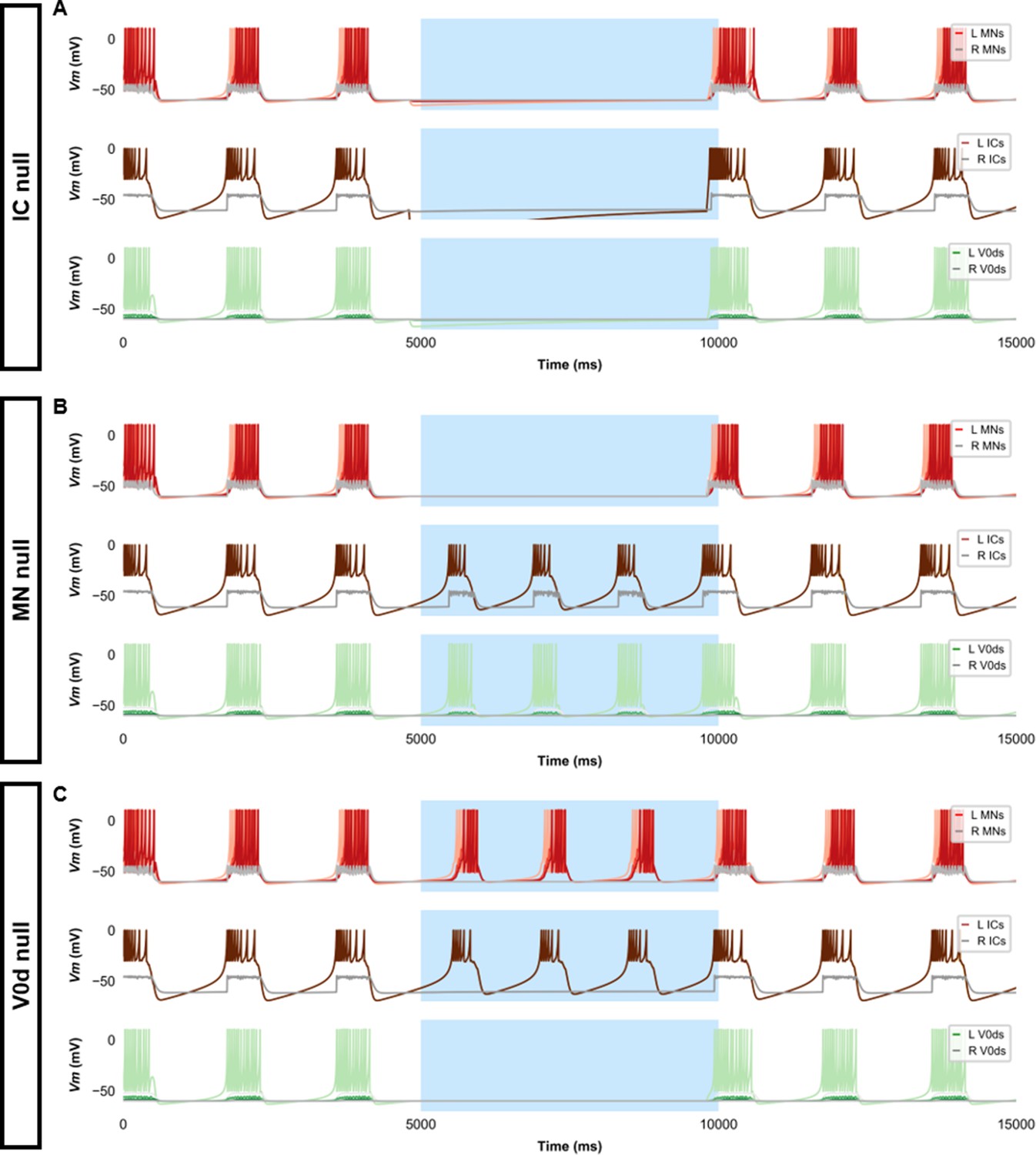
Silencing spinal neurons during single coiling.
Simulations consisted of three 5000 ms epochs. In the middle epoch, silencing of targeted spinal neurons was achieved by removing all synaptic and external currents from the targeted population. Synaptic and external currents were restored in the last epoch. (A) Silencing IC neurons silences the other spinal neurons. (B) Silencing MNs slightly reduces IC burst duration but does not preclude IC bursting. (C) Silencing V0ds blocks synaptic bursts in contralateral ICs and MNs but does not preclude single coils, nor does it lead to multiple coils. The Vm of a rostral (lightest), middle, and caudal (darkest) neuron is shown, except for IC neurons that are all in a rostral kernel. L: left, R: right. IC, Ipsilateral Caudal; MN, motoneuron.
Figure 2—figure supplement 2
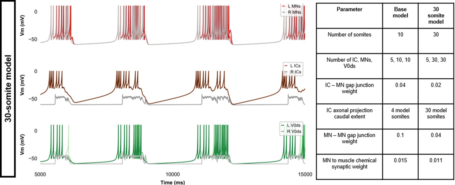
Membrane potential (Vm) during a simulation of a 30-somite single coiling model.
The Vm of a rostral (lightest), middle, and caudal (darkest) neuron is shown, except for IC neurons that are all in a rostral kernel. L: left, R: right. IC, Ipsilateral Caudal.
Figure 2—video 1
Single coiling model.
Figure 2—video 2
Truncated coils.
Figure 3 with 7 supplements
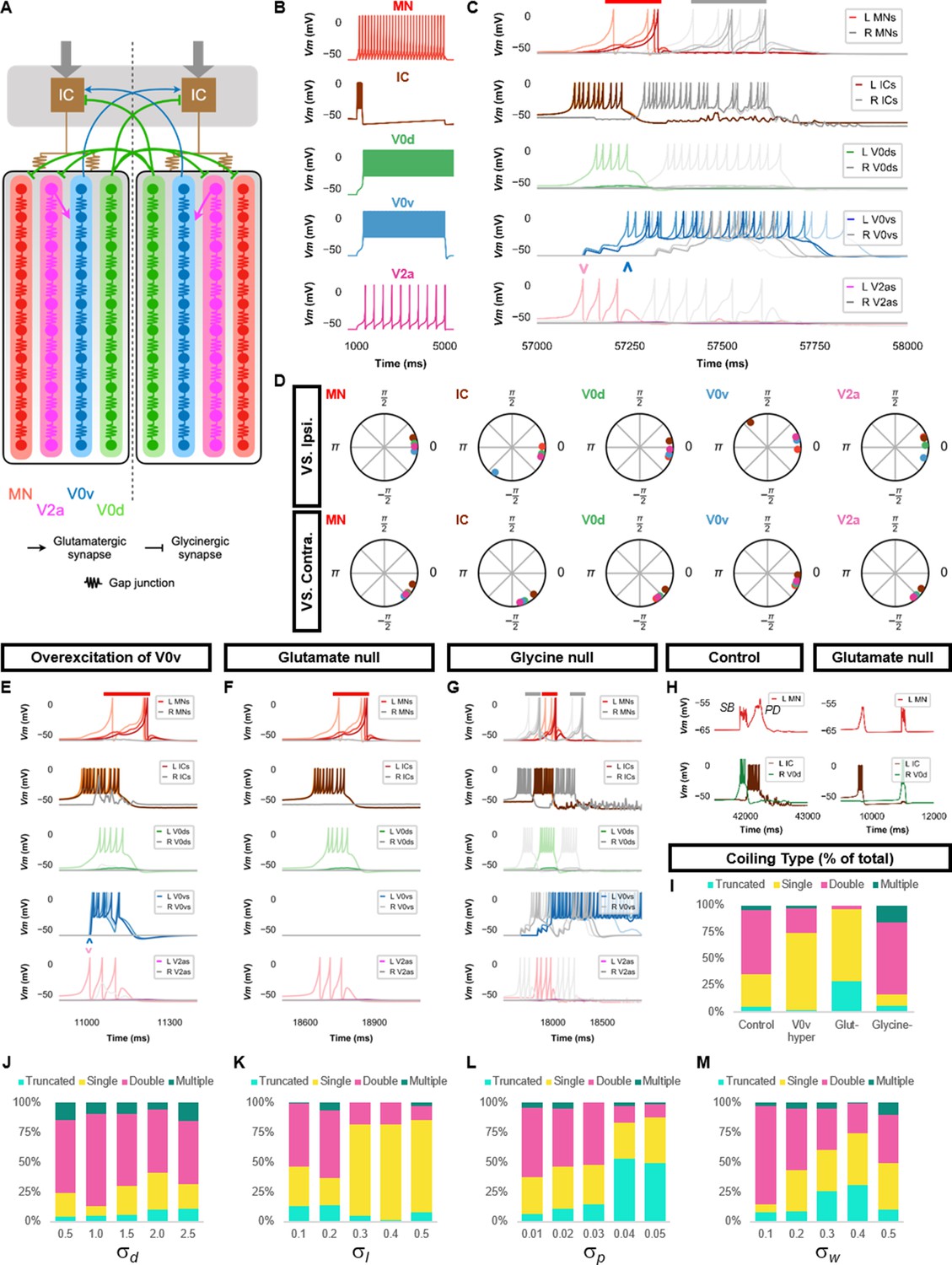
Double coiling model relies on a hybrid network of electrical and chemical synapses.
(A) Schematic of the double coiling model. Gap junctions between spinal neurons are not depicted. Dashed line indicates the body midline. Gray arrows indicate descending motor command. (B) Membrane potential (Vm) response of isolated spinal neuron models to a depolarizing current step. (C) Vm of spinal neurons during a double coil. (D) The phase delay of left neurons in relation to ipsilateral and contralateral spinal neurons in the fifth somite and an IC in the rostral kernel during five consecutive left-right double coils. The reference neuron for each polar plot is labeled, and all neurons follow the same color-coding as the rest of the figure. A negative phase delay indicates that the reference neuron precedes the neuron to which it is compared. A phase of 0 indicates that a pair of neurons is in-phase; a phase of π indicates that a pair of neurons is out-of-phase. Vm in simulations where (E) the weights of the V2a to V0v and the V0v to IC synapses were increased to show that early excitation of V0v prevented the initiation of a second coil following a single coil, (F) all glutamatergic transmission was blocked, and (G) glycinergic transmission was blocked. (H) Top row, mixed event composed of a synaptic burst (SB) directly followed by a periodic depolarization (PD) in a motoneuron in control but not in glutamate null conditions. Bottom row, Vm in left IC and right V0d during events in top row. (I) Proportions of single, double, multiple, and truncated coiling events under control, glutamate null (Glut−), overexcited V0vs (V0v hyper), and glycine null (Glycine-) conditions. Each condition was tested with five 100,000 ms runs with = 0.5, =0.01, and = 0.05. (J–M) Sensitivity testing showing proportions of single, double, multiple, and truncated coiling events during ten 100,000 ms runs for each value of , , , and tested. Solid red and gray bars in (C,E–G) indicate the duration of coils. Chevrons in (C and E) denote the initial spiking of V0vs and V2as to indicate latency of V0v firing during the first coil. For (C, E–G), the Vm of a rostral (lightest), middle, and caudal (darkest) neuron is shown, except for IC neurons that are all in a rostral kernel. L: left, R: right. See also Figure 3—figure supplements 1 and 2 and Figure 3—videos 1–4. IC, Ipsilateral Cauda; MN, motoneuron.
Figure 3—figure supplement 1
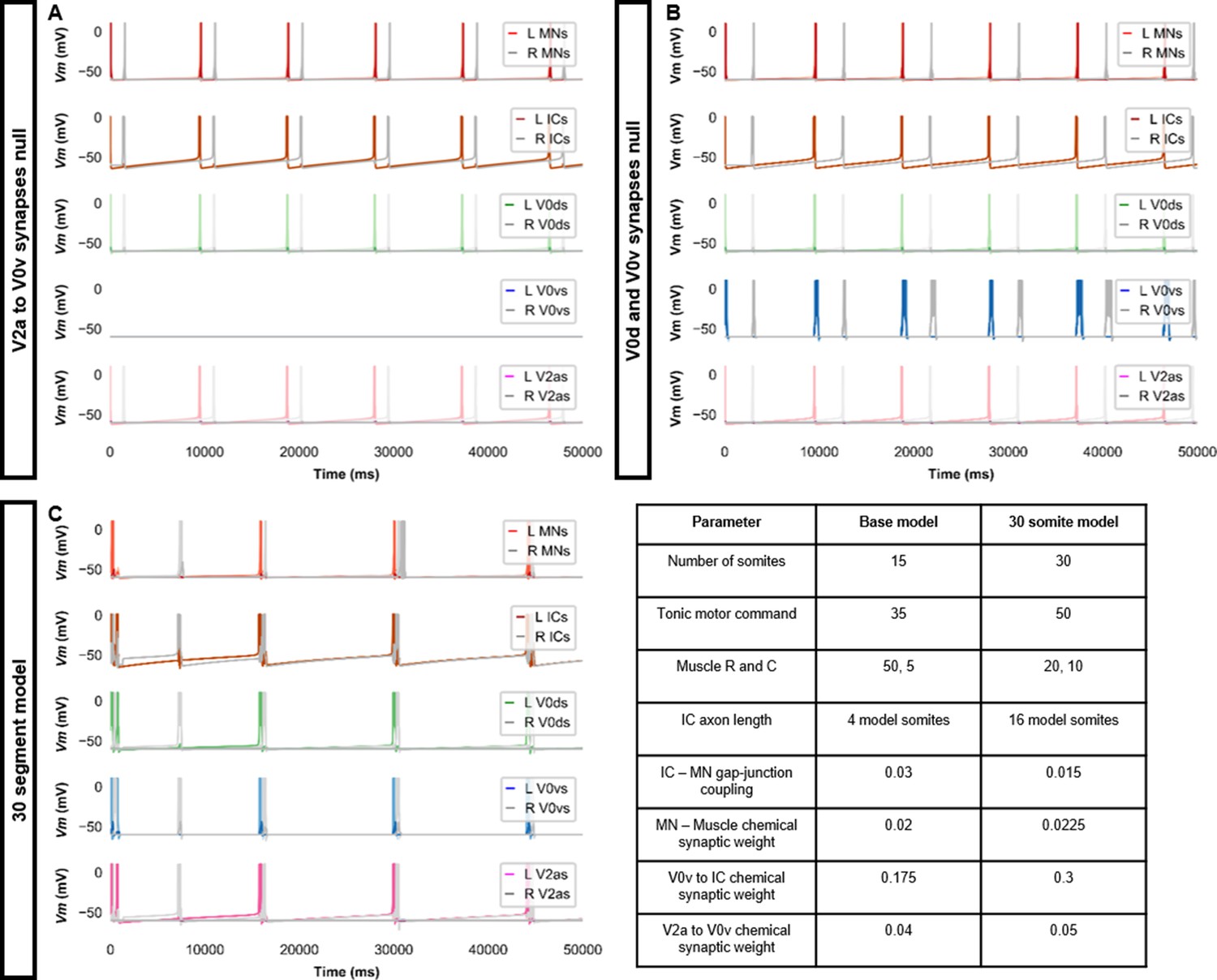
Double coiling model with no V2a to V0v synapses, no contralateral synapses, or with 30 somites.
(A) Membrane potential (Vm) during a simulation without V2a to V0v synapses. V0v neurons remain inactive, and there are only single coils. (B) Simulation with no contralateral inhibition or excitation. The lack of double and multiple coils, even without contralateral inhibition, suggests that contralateral excitation is necessary to generate double and multiple coils. (C) Double coiling in a model composed of 30 somites. The Vm of a rostral (lightest), middle, and caudal (darkest) neuron is shown, except for IC neurons that are all in a rostral kernel. L: left, R: right. See also Figure 3—video 5. IC, Ipsilateral Caudal; MN, motoneuron.
Figure 3—figure supplement 2
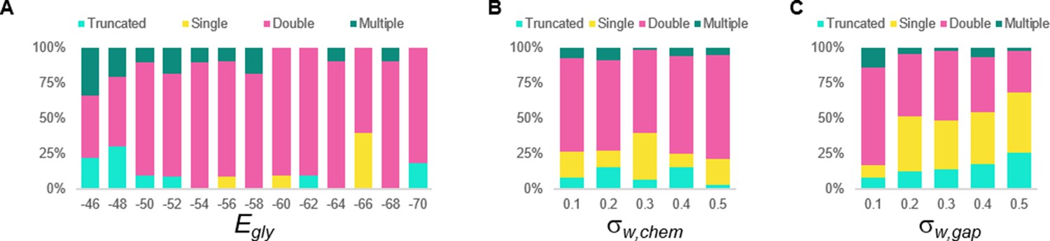
Sensitivity testing of the double coiling model for the glycinergic reversal potential (Egly), weights of chemical synapses (σw, chem), and weights of gap junctions (σw, gap).
Sensitivity testing showing proportions of single, double, multiple, and truncated coiling events during ten 100,000 ms runs for each value tested.
Figure 3—video 1
Double coiling model.
Figure 3—video 2
Glutamate null double coiling model.
Figure 3—video 3
Overexcited V0v double coiling model.
Figure 3—video 4
Glycine null double coiling model.
Figure 3—video 5
30-somite double coiling model.
Figure 4 with 1 supplement
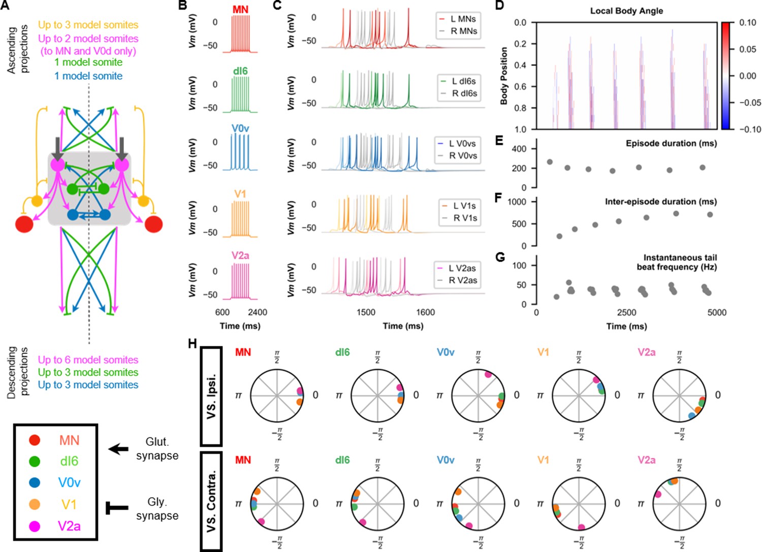
The base model for beat-and-glide swimming.
(A) Schematic of the model architecture underlying beat-and-glide swimming. (B) Membrane potential (Vm) response to a depolarizing current step of isolated spinal neurons in the model. (C) Vm of spinal neurons during a beat-and-glide swimming simulation. The Vm of a rostral (lightest), middle, and caudal (darkest) neuron is shown. L: left, R: right. (D) Heat-map of local body angle. (E) Episode duration, (F) inter-episode interval, (G) instantaneous tail beat frequency, and (H) the phase delay of left neurons in relation to ipsilateral and contralateral spinal neurons in the 10th somite during a 10,000 ms simulation. The reference neuron for each polar plot is labeled, and all neurons follow the same color-coding as the rest of the figure. A negative phase delay indicates that the reference neuron precedes the neuron to which it is compared. A phase of 0 indicates that a pair of neurons is in-phase; a phase of π indicates that a pair of neurons is out-of-phase. See also Figure 4—video 1. IC, Ipsilateral Caudal; MN, motoneuron.
Figure 4—video 1
Beat-and-glide model.
Figure 5 with 3 supplements
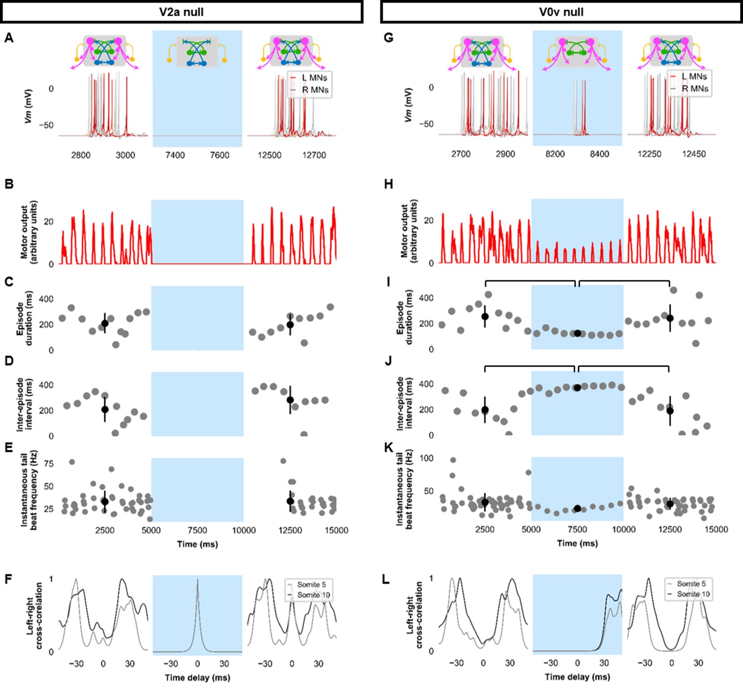
Silencing spinal excitatory neurons during beat-and-glide swimming.
Simulations consisted of three 5,000 ms epochs. In the middle epoch, silencing of targeted spinal neurons was achieved by removing all synaptic and external currents from the targeted population. Synaptic and external currents were restored in the last epoch. (A–F) Simulations where V2as were silenced and (G–L), where V0vs were silenced. (A, G) Top, the functional state of the spinal network during the three epochs. Bottom, motoneuron (MN) membrane potential (Vm) during simulations where targeted neurons were silenced in the middle epoch. The Vm of a rostral (lightest), middle, and caudal (darkest) neuron is shown. (B, H) The integrated muscle output, (C, I) episode duration, (D, J) inter-episode intervals, and (E, K) instantaneous tail beat frequency during each respective simulation. Averages within epoch are shown in black (mean±s.d.). Brackets denote significant pairwise differences. (F, L) The left-right coordination of somites 5 and 10. L: left, R: right. The first part of epoch 3 of the V2a silenced simulation involved synchronous left-right activity, hence the lack of instantaneous tail beat frequency values. Statistics: For (C–E), there were no episodes during epoch 2. There were no statistically significant differences between epochs 1 and 3 for any of the parameters. (I) F2,31=7.2, p=0.0029. (J) F2,28=10.2, p=0.001. (K) F2,115=3.0, p=0.055. P-values for t-tests are found in Figure 5—source data 1. See also Figure 5—figure supplement 1 and Figure 5—videos 1 and 2. MN, motoneuron.
-
Figure 5—source data 1
P-values for V2a null and V0v null simulations.
- https://cdn.elifesciences.org/articles/67453/elife-67453-fig5-data1-v2.xlsx
Figure 5—figure supplement 1
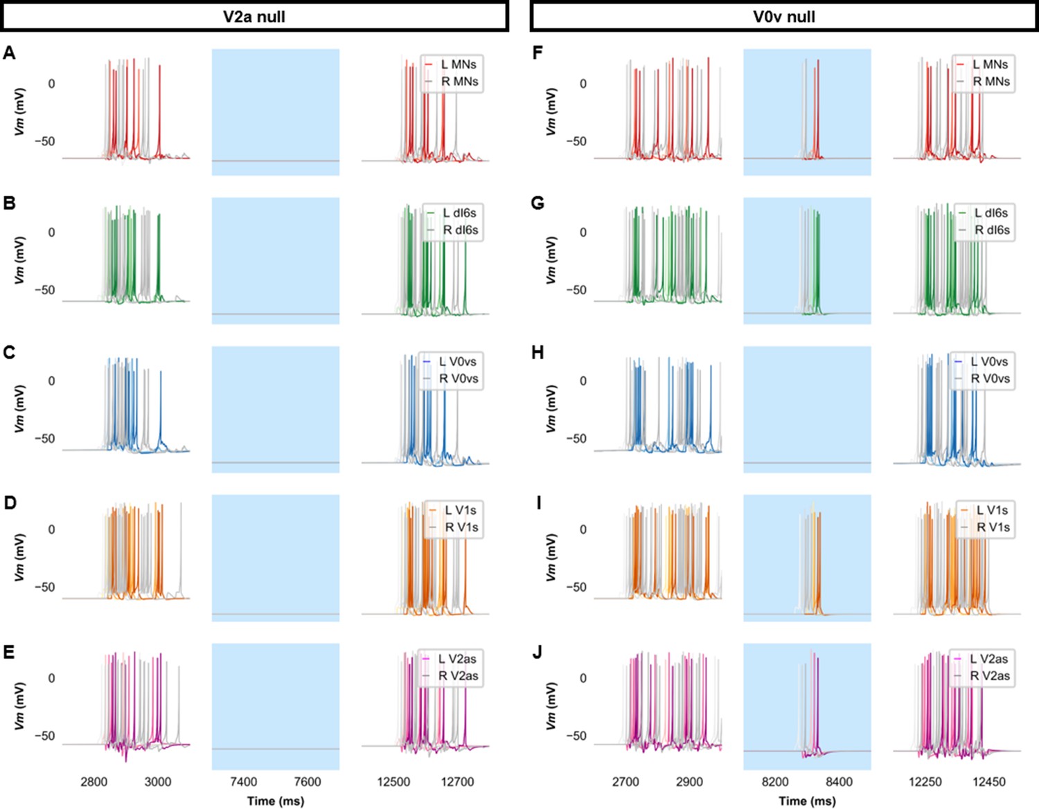
Membrane potential (Vm) of spinal neurons during simulations of beat-and-glide swimming where excitatory neurons were silenced.
Simulations consisted of three 5000 ms epochs. In the middle epoch, silencing of targeted spinal neurons was achieved by removing all synaptic and external currents from the targeted population. Synaptic and external currents were restored in the last epoch. (A–E) Simulations where V2as were silenced and (F–J), where V0vs were silenced in the middle epoch. The Vm of a rostral (lightest), middle, and caudal (darkest) neuron is shown. L: left, R: right. MN, motoneuron.
Figure 5—video 1
V2a knockout beat-and-glide model.
Figure 5—video 2
V0v knockout beat-and-glide model.
Figure 6 with 4 supplements
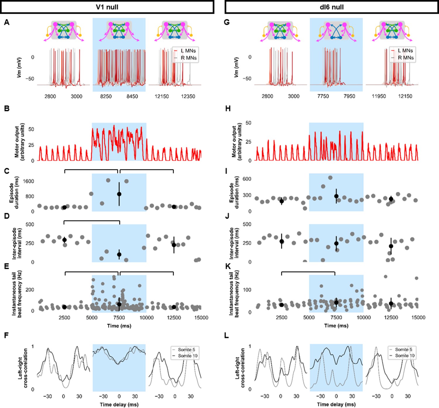
Silencing spinal inhibitory neurons during beat-and-glide swimming.
Simulations consisted of three 5000 ms epochs. In the middle epoch, silencing of targeted spinal neurons was achieved by removing all synaptic and external currents from the targeted population. Synaptic and external currents were restored in the last epoch. (A–F) Simulations where V1s were silenced and (G–L), where dI6s were silenced. (A, G) Top, the functional state of the spinal network during the three epochs. Bottom, motoneuron (MN) membrane potential (Vm) during simulations where targeted neurons were silenced in the middle epoch. The Vm of a rostral (lightest), middle, and caudal (darkest) neuron is shown. (B, H) The integrated muscle output, (C, I) episode duration, (D, J) inter-episode intervals, and (E, K) instantaneous tail beat frequency during each respective simulation. Averages within epoch are shown in black (mean±s.d.). Brackets denote significant pairwise differences. (F, L) The left-right coordination of somites 5 and 10. L: left, R: right. Statistics: (C) F2,25=10.5, p=5.8×10⁻⁴. (D) F2,22=6.6, p=0.0063. (E) F2,214=6.9, p=0.0013. (I) F2,31=2.5 p=0.10. (J) F2,28=0.9, p=0.42. (K) F2,145=3.5, p=0.033. P-values for t-tests are found in Figure 6—source data 1. See also Figure 6—figure supplements 1 and 2 and Figure 6—videos 1 and 2.
-
Figure 6—source data 1
P-values for V1 null and dI6 null simulations.
- https://cdn.elifesciences.org/articles/67453/elife-67453-fig6-data1-v2.xlsx
Figure 6—figure supplement 1
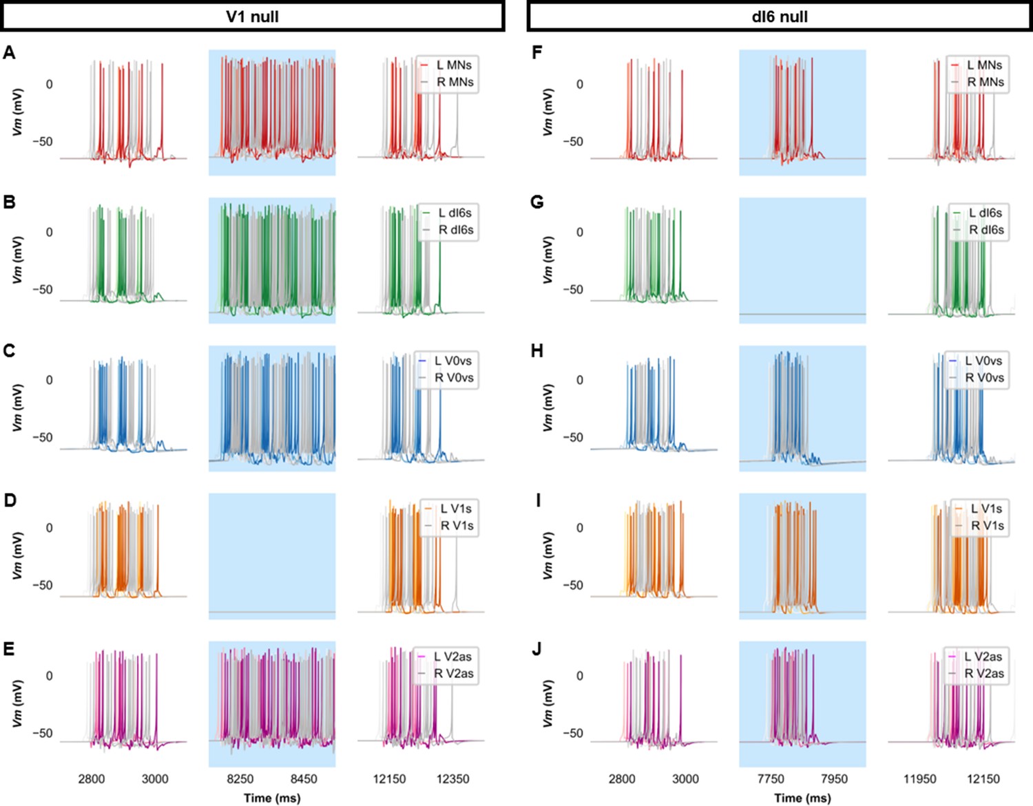
Membrane potential (Vm) of spinal neurons during simulations of beat-and-glide swimming where inhibitory neurons were silenced.
Simulations consisted of three 5000 ms epochs. In the middle epoch, silencing of targeted spinal neurons was achieved by removing all synaptic and external currents from the targeted population. Synaptic and external currents were restored in the last epoch. (A–E) Simulations where V1s were silenced and (F–J), where dI6s were silenced in the middle epoch. The Vm of a rostral (lightest), middle, and caudal (darkest) neuron is shown. L: left, R: right. MN, motoneuron.
Figure 6—figure supplement 2
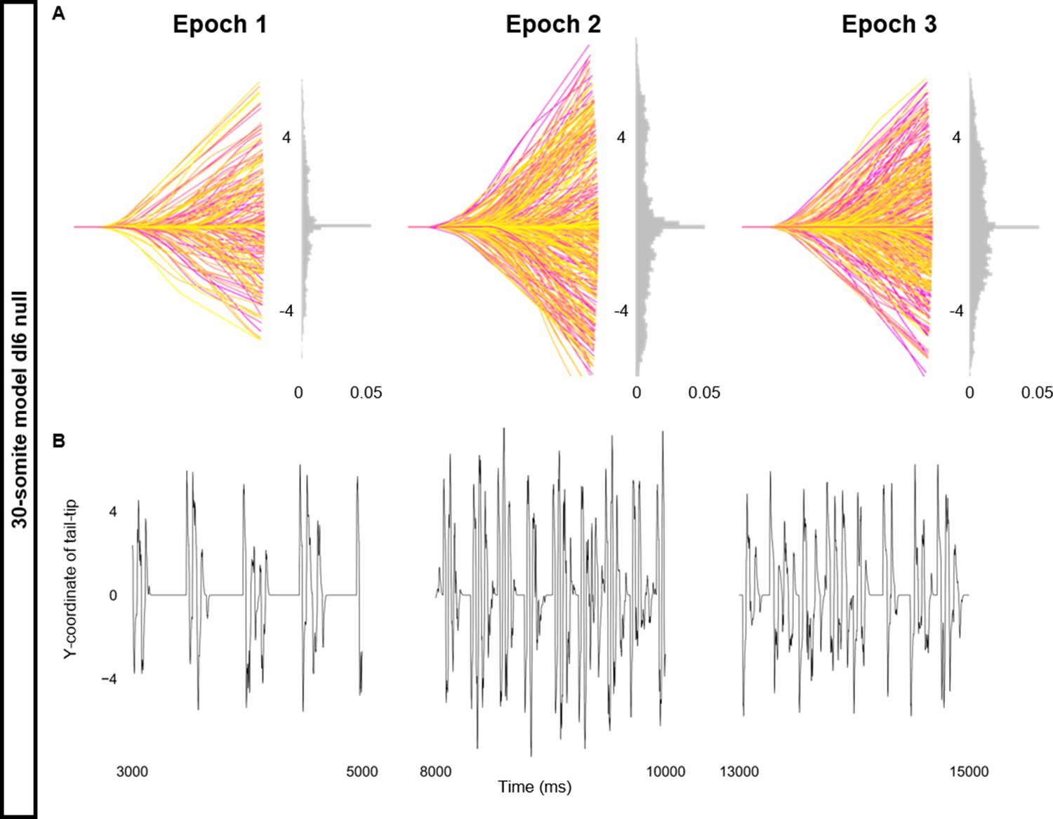
Altered kinematics during silencing of dI6 neurons.
Simulation of a 30-somite beat-and-glide swimming model consisted of three 5000 ms epochs. In the middle epoch, silencing of dI6s was achieved by removing all synaptic and external currents from the targeted population. Synaptic and external currents were restored in the last epoch. (A) Representative body midlines are shown for each epoch along with a probability density histogram of the y-coordinate of the terminal somite during each epoch. The histograms are truncated at 0.05 as there were many points at y=0 during inter-episode intervals. The magenta to yellow color coding represents the progression through each epoch. (B) Y-coordinate of the tail tip during the last 2000 ms of each epoch. Details of the 30-somite model are described in Figure 8—figure supplement 1.
Figure 6—video 1
V1 knockout beat-and-glide model.
Figure 6—video 2
dI6 knockout beat-and-glide model.
Figure 7 with 2 supplements
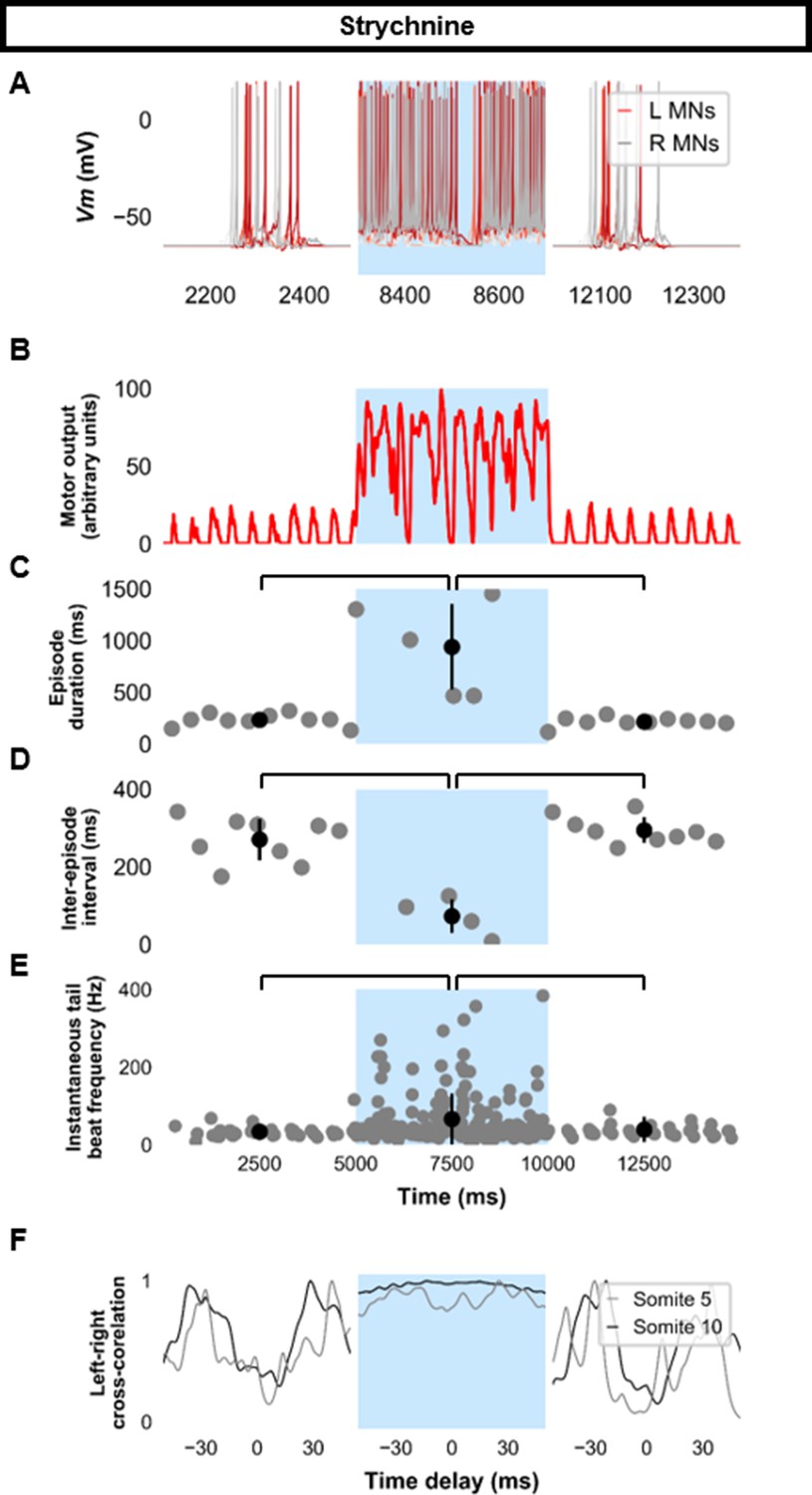
Simulating the effects of strychnine on beat-and-glide swimming.
Simulations to assess the effects of blocking glycinergic transmission consisted of three 5000 ms epochs. In the middle epoch, all glycinergic currents were blocked. Glycinergic transmission was restored in the last epoch. (A) Motoneuron (MN) membrane potential (Vm) during simulations where glycinergic transmission was blocked in the middle epoch. The Vm of a rostral (lightest), middle, and caudal (darkest) neuron is shown. (B) The integrated muscle output, (C) episode duration, (D) inter-episode intervals, and (E) instantaneous tail beat frequency during this simulation. Averages within epoch are shown in black (mean±s.d.). (F) The left-right coordination of somites 5 and 10. L: left, R: right. Statistics: (C) F2,24=2.5, p=2.2×10⁻⁶. (D) F2,21=32.0, p=8.3×10⁻⁷. (E) F2,267=8.3, p=0.0003. P-values for t-tests are found in Figure 7—source data 1. See also Figure 7—figure supplement 1 and Figure 7—video 1.
-
Figure 7—source data 1
P-values for strychnine simulations.
- https://cdn.elifesciences.org/articles/67453/elife-67453-fig7-data1-v2.xlsx
Figure 7—figure supplement 1
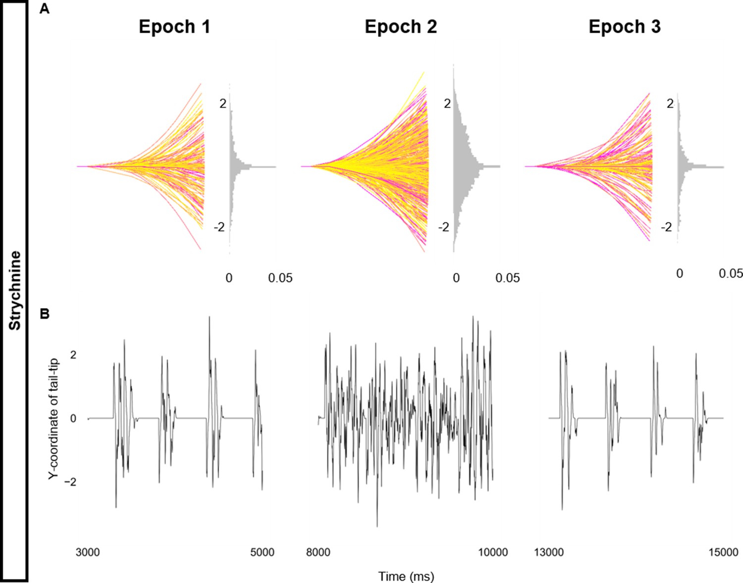
Altered kinematics during strychnine.
Simulation of the base beat-and-glide swimming model consisted of three 5000 ms epochs. In the middle epoch, all glycinergic currents were blocked. Glycinergic transmission was restored in the last epoch. (A) Representative body midlines are shown for each epoch along with a probability density histogram of the y-coordinate of the terminal somite during each epoch. The histograms are truncated at 0.05 as there were many points at y=0 during inter-episode intervals. The magenta to yellow color coding represents the progression through each epoch. (B) Y-coordinate of the tail tip during the last 2000 ms of each epoch.
Figure 7—video 1
Glycine null beat-and-glide model.
Figure 8 with 5 supplements
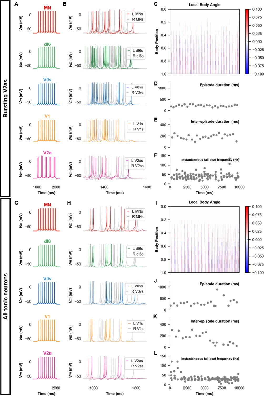
Beat-and-glide models with bursting V2a (A–F) or only tonic neurons (G–L).
(A, G) Membrane potential (Vm) response of isolated neurons in the model to a current step. (B, H) Vm of spinal neurons during swimming simulation. The membrane potential of a rostral (lightest), middle, and caudal (darkest) neuron is shown. L: left, R: right. (C, I) Heat-map of local body angle. (D, J) Episode duration, (E, K) inter-episode interval, and (F, L) instantaneous tail beat frequency during the same simulations as (B and H), respectively. See also Figure 8—figure supplements 1 and 2 and Figure 8—videos 1 and 2. MN, motoneuron.
-
Figure 8—source data 1
P-values for sensitivity testing to values of E_gly.
- https://cdn.elifesciences.org/articles/67453/elife-67453-fig8-data1-v2.xlsx
Figure 8—figure supplement 1
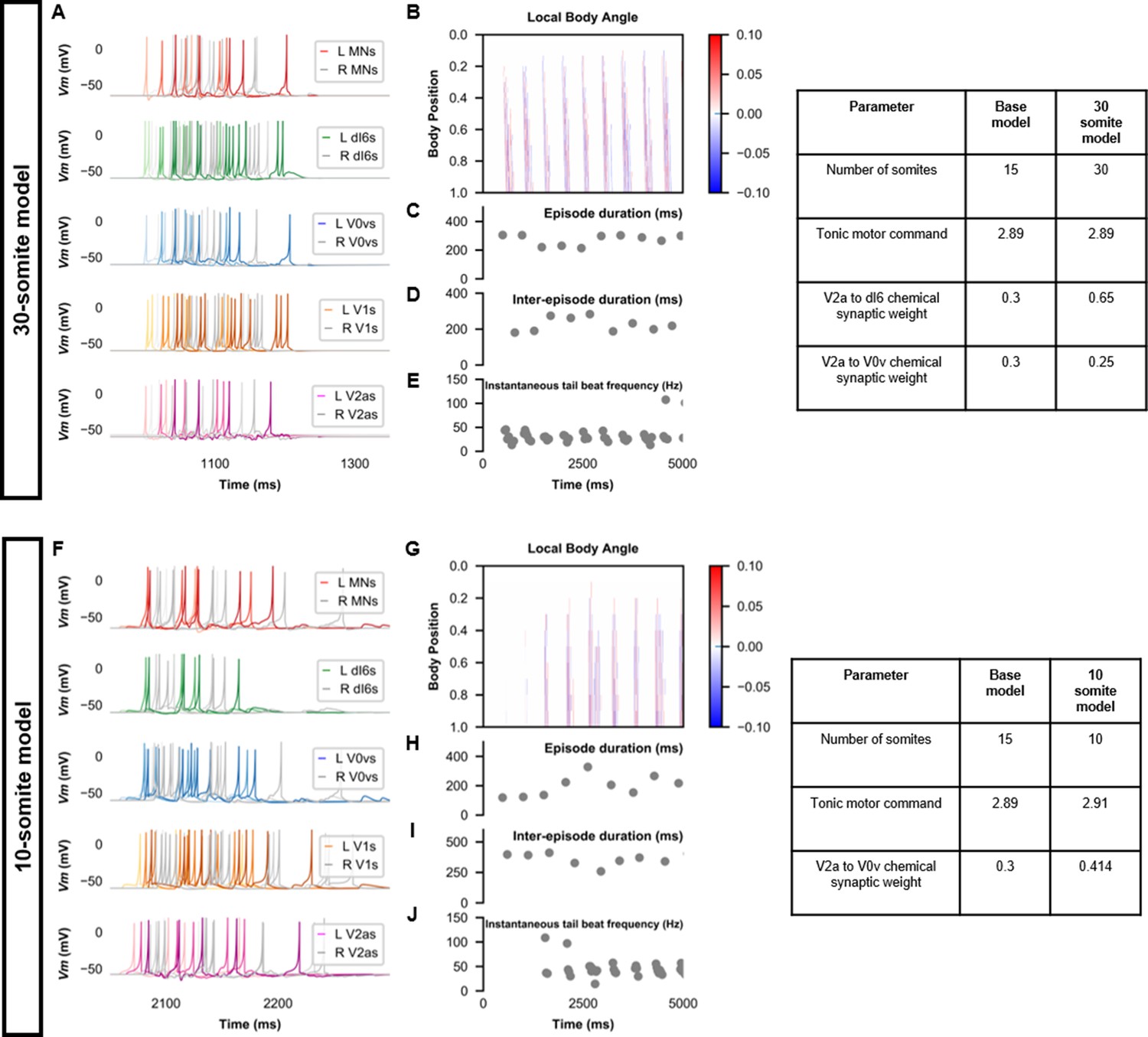
Beat-and-glide swimming model with different number of somites.
(A, F) Membrane potential (Vm) of spinal neurons during a beat-and-glide swimming simulation. The Vm of a rostral (lightest), middle, and caudal (darkest) neuron is shown. L: left, R: right. (B, G) Heat-map of local body angle, (C, H) episode duration, (D, I) inter-episode interval, and (E, J) instantaneous tail beat frequency during the same simulations as (A and F), respectively. MN, motoneuron.
Figure 8—figure supplement 2
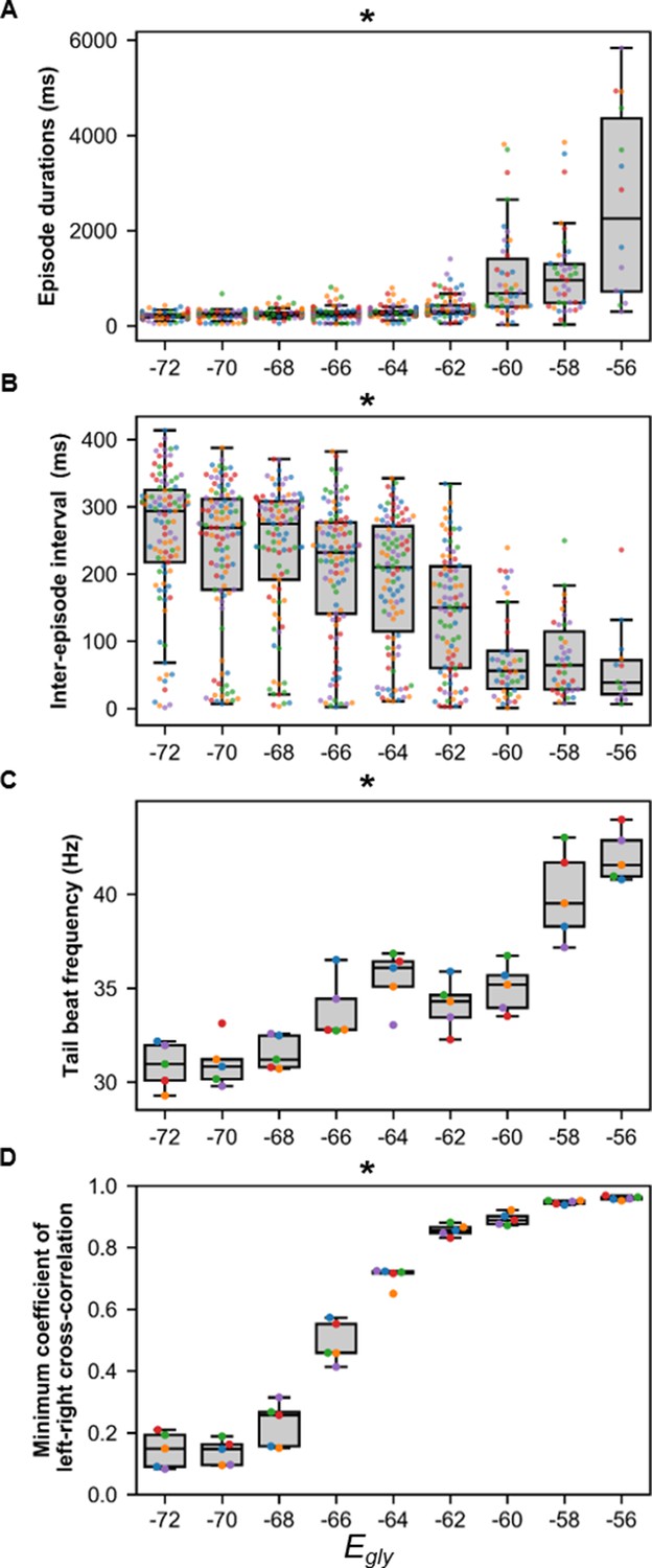
Sensitivity of beat-and-glide swimming to variability in glycinergic reversal potential (Egly).
Five 10,000 ms long simulations were run for each value of Egly. (A) Episode duration, (B) inter-episode intervals, and (C) average tail beat frequency during each swimming episode. (D) The minimum coefficient of the cross-correlation of left and right muscle was calculated at each Egly. The minimum coefficient was taken between −10 and 10 ms time delays. Asterisks denote significant differences detected using a one-factor ANOVA test. Each run is color-coded. Statistics: (A) F8,681=74.9, p=2.7×10−88. (B) F8,681=32.6, p=1.5×10−43. (C) F8,36=22.9, p=6.0×10⁻¹². (D) F8,36=327.8, p=3.0×10⁻³¹. P-values for t-tests are found in Figure 8—source data 1.
Figure 8—video 1
Beat-and-glide with bursting V2a model.
Figure 8—video 2
Swimming model with only tonic neurons.
Figure 8—video 3
30-somite beat-and-glide model.
Figure 9
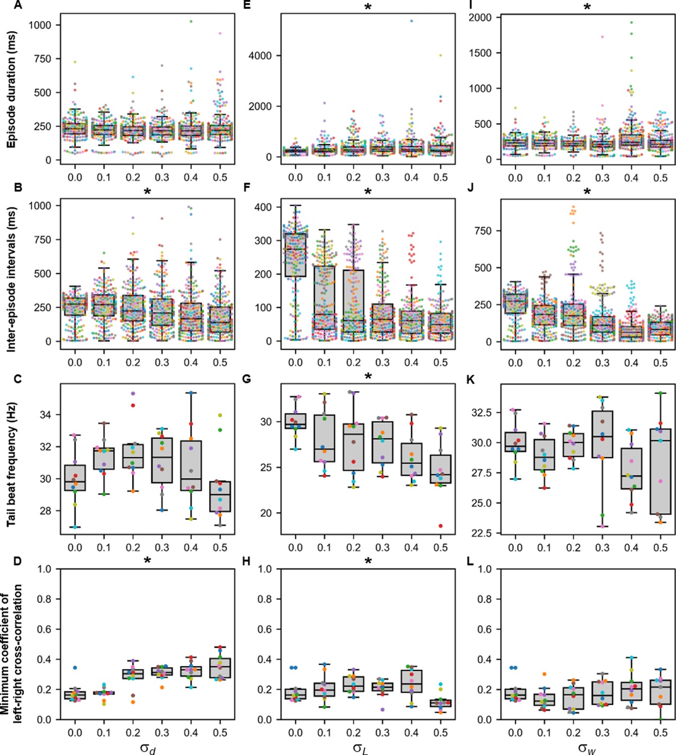
Sensitivity of beat-and-glide swimming to tonic motor command amplitude, length of rostrocaudal projections, and synaptic weighting.
Ten 10,000-ms long simulations were run for each value of (A–D), (E–H), and (I–L) tested. (A, E, I) Episode duration. (B, F, J) Inter-episode interval. (C, G, K) Average tail beat frequency during each swimming episode. (D, H, L) Minimum coefficient of the cross-correlation of left and right muscle. The minimum was taken between −10 and 10 ms time delays. Each circle represents a single swimming episode (A, E, I), inter-episode interval (B, F, J), or a single run (all other panels). Each run is color-coded. Runs with only one side showing activity are not depicted in (D and H). Asterisks denote significant differences detected using a one-factor ANOVA test. Statistics: (A) F5,1253=2.5, p=0.03. (Note that there were no pairwise differences detected). (B) F5,1253=11.2, p=1.3×10⁻¹⁰. (C) F5,54=1.9, p=0.11. (D) F5,54= 14.5, p=5.2×10⁻⁹. (E) F5,1253=8.7, p=3.8×10⁻⁸. (F) F5,1253=118.1, p=2.0×10−102. (G) F5,54=4.0, p=0.004. (H) F5,54=3.2, p=0.014. (I) F5,1400=13.5, p=6.8×10⁻¹³. (J) F5,1400=74.5, p=2.5×10−69. (K) F5,53=1.3, p=0.30. (L) F5,53=0.8, p=0.55. P-values for t-tests are found in Figure 9—source data 1.
-
Figure 9—source data 1
P-values for sensitivity testing to values of sigma D, L and W.
- https://cdn.elifesciences.org/articles/67453/elife-67453-fig9-data1-v2.xlsx
Figure 10
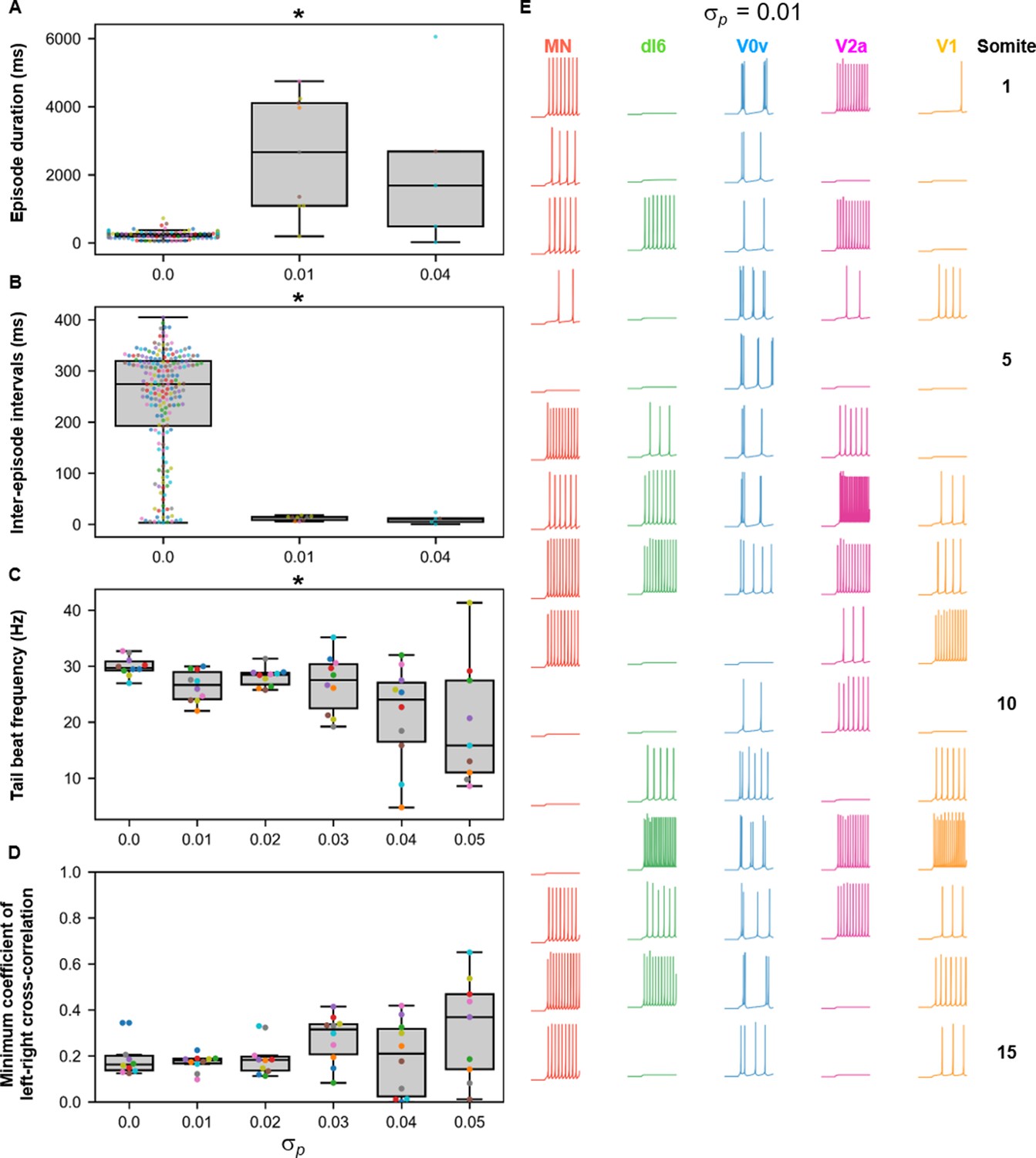
Sensitivity of beat-and-glide swimming to variability in membrane potential dynamics.
Ten 10,000-ms long simulations were run at each value of (A–D). (A) Episode duration. (B) Inter-episode interval. (C) Average tail beat frequency during each swimming episode. (D) Minimum coefficient of the cross-correlation of left and right muscle. The minimum was taken between −10 and 10 ms time delays. Each circle represents a single swimming episode (A), inter-episode interval (B), or a single run (C, D). Each run is color-coded. Runs not depicted exhibited either continual motor activity with no gliding pauses or no swimming activity. Asterisks denote significant differences detected using a one-factor ANOVA test. (E) Responses to a 1-s long step current of all neurons on the left side in a model where =0.01. Step current amplitudes varied between populations of neurons. The amplitude of the step currents to each population is the same as in Figure 4B. The simulation of the model with these neurons generated continued swimming activity with no gliding pauses. The neurons are ordered by somite, from somite 1 at the top to somite 15 at the bottom. Statistics: (A) F2,211=143.8, p=4.0×10−40. (B) F2,211=32.3, p=5.8×10⁻¹³. (C) F5,53=4.0, p=0.0036. (D) F5,53=2.1, p=0.085. P-values for t-tests are found in Figure 10—source data 1. MN, motoneuron.
-
Figure 10—source data 1
P-values for sensitivity testing to values of Sigma P.
- https://cdn.elifesciences.org/articles/67453/elife-67453-fig10-data1-v2.xlsx
Figure 11 with 1 supplement
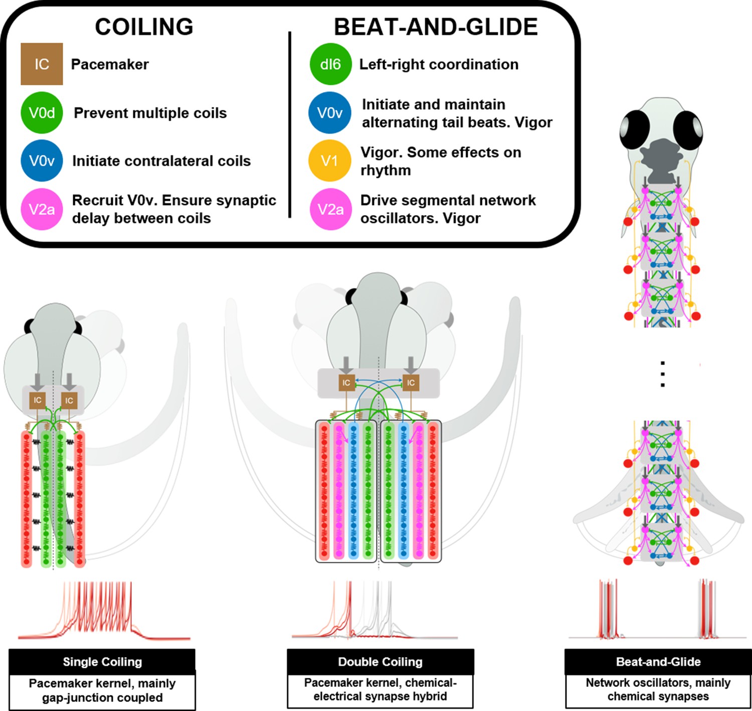
Summary figure of computational models of zebrafish locomotor movements during development.
See also Figure 11—video 1.
Figure 11—video 1
Summary of developmental zebrafish computational models.
Tables
Table 1
Electrical synapse (gap junctions) weights between neuron populations.
| Coiling Beat-and-glide | MN | IC | V0d dI6 | V0v | V2a |
|---|---|---|---|---|---|
| MN Single coiling Double coiling Beat-and-glide (all models) | 0.1 0.07 0.005 | ||||
| IC Single coiling Double coiling | 0.04 0.03 | 0.001 0.0001 | |||
| V0d or dI6 Single coiling Double coiling Beat-and-glide (all models) | 0.01 0.0001 0.0001 | 0.05 0.05 | 0.04 0.04 0.04 | ||
| V0v Double coiling Beat-and-glide (all models) | 0.0001 0.005 | 0.0005 | 0.05 0.05 | ||
| V2a Double coiling Beat-and-glide (all models) | 0.005 0.005 | 0.15 | 0.005 0.005 |
Table 2
Glutamatergic and glycinergic reversal potentials and time constants.
| Chemical synapse | Erev | τr | τf | Vthr |
|---|---|---|---|---|
| Glutamatergic | 0 | 0.5 | 1.0 | −15 |
| Glycinergic | −45, –58, −70* | 0.5 | 1.0 | −15 |
-
*For single and double coiling and beat-and-glide swimming models, respectively.
Table 3
Chemical synapse weights between neuron populations.
Pre-synaptic neurons are in rows. Post-synaptic neurons in columns.
| Pre-synaptic | Post-synaptic | ||||||
|---|---|---|---|---|---|---|---|
| MN | IC | V0d dI6 | V0v | V2a | V1 | Muscle | |
| MN Single coiling Double coiling Beat-and-glide (all models) | 0.015 0.02 0.1 | ||||||
| V0d Single coiling Double coiling | 0.3 2.0 | 0.3 2.0 | | 2.0 | |||
| dI6 Beat-and-glide (base) Beat-and-glide (bursting V2a) Beat-and-glide (all tonic neurons) | 1.5 1.5 1.5 | 0.25* 0.25* 0.25* | 1.5 2.0 1.5 | ||||
| V0v Double coiling Beat-and-glide (base) Beat-and-glide (bursting V2a) Beat-and-glide (all tonic neurons) | 0.175 | 0.4 0.75 0.4 | |||||
| V2a Double coiling Beat-and-glide (base) Beat-and-glide (bursting V2a) Beat-and-glide (all tonic neurons) | 0.5 0.5 0.5 | 0.5 0.75 0.5 | 0.04 0.3 0.275 0.25 | 0.3 0.3 0.3 | 0.5 0.5 0.5 | ||
| V1 Beat-and-glide (base) Beat-and-glide (bursting V2a) Beat-and-glide (all tonic neurons) | 1.0 1.0 1.0 | 0.2 0.2 0.2 | 0.1 0.1 0.1 | 0.5 0.5 0.6 | |||
-
*Scaled by a random number selected from a gaussian distribution with mean of 1 and variance of 0.1.
Table 4
Parameter values of neurons.
| Model population | a | b | c | d | Vmax | Vr | Vt | k | C | Rostro-caudal position* | Idrive† |
|---|---|---|---|---|---|---|---|---|---|---|---|
| MN Single coiling Double coiling Beat-and-glide | 0.5 0.5 0.5 | 0.1 0.1 0.01 | −50 −50 −55 | 0.2 100 100 | 10 10 10 | −60 −60 −65 | −45 −50 −58 | 0.05 0.05 0.5 | 20 20 20 | 5.0+1.6*n | |
| IC Single coiling Double coiling | 0.0005 0.0002 | 0.5 0.5 | −30 −40 | 5 5 | 0 0 | −60 −60 | −45 −45 | 0.05 0.03 | 50 50 | 1.0 | 50 35 |
| V0d Single coiling Double coiling | 0.5 0.02 | 0.01 0.1 | −50 −30 | 0.2 3.75 | 10 10 | −60 −60 | −45 −45 | 0.05 0.09 | 20 6 | 5.0+1.6*n | |
| dI6 Beat-and-glide (all models) | 0.1 | 0.002 | −55 | 4 | 10 | −60 | −54 | 0.3 | 10 | 5.1+1.6*n | |
| V0v Double coiling Beat-and-glide (base) Beat-and-glide (bursting V2a and all tonic models) | 0.02 0.01 0.1 | 0.1 0.002 0.002 | −30 −55 −55 | 11.6 8 4 | 10 10 10 | −60 −60 −60 | −45 −54 −54 | 0.05 0.3 0.3 | 20 10 10 | 5.1+1.6*n | |
| V2a Double coiling Beat-and-glide (base and all tonic models) Beat-and-glide (bursting V2a model) | 0.5 0.1 0.01 | 0.1 0.002 0.002 | −40 −55 −55 | 100 4 8 | 10 10 10 | −60 −60 −60 | −45 −54 −54 | 0.05 0.3 0.3 | 20 10 10 | 5.1+1.6*n | 2.89 3.05 |
| V1 Beat-and-glide (all models) | 0.1 | 0.002 | −55 | 4 | 10 | −60 | −54 | 0.3 | 10 | 7.1+1.6*n |
-
*n=0 to N−1, N being the total number of neurons in that given population.
†Amplitude of tonic motor command drive.
Table 5
Comparison of beat-and-glide swimming in model and experimental data from Buss and Drapeau, 2001.
| Parameter | Base model | Buss and Drapeau, 2001 |
|---|---|---|
| Mean episode duration (ms) | 234±6 | 180±20 |
| Mean inter-episode interval (ms) | 242±20 | 390±30 |
| Mean tail beat frequency (Hz) | 30.0±0.6 | 35±2 |
-
Values in mean± standard error. n=ten 10,000 ms-long simulations for the base model, and n=12 animals for the data from Buss and Drapeau, 2001.
Key resources table
| Reagent type (species) or resource | Designation | Source or reference | Identifiers | Additional information |
|---|---|---|---|---|
| Software, algorithm | Python | Python | RRID:SCR_008394 |
Additional files
Download links
A two-part list of links to download the article, or parts of the article, in various formats.
Downloads (link to download the article as PDF)
Open citations (links to open the citations from this article in various online reference manager services)
Cite this article (links to download the citations from this article in formats compatible with various reference manager tools)
Modeling spinal locomotor circuits for movements in developing zebrafish
eLife 10:e67453.
https://doi.org/10.7554/eLife.67453


