Figures and data in Quantifying the relationship between genetic diversity and population size suggests natural selection cannot explain Lewontin’s Paradox

Version of Record

Accepted for publication after peer review and revision.

Download
Cite
Share
CommentOpen annotations (there are currently 0 annotations on this page).

Version of Record published: October 1, 2021 (This version)
Accepted Manuscript updated: August 31, 2021 (Go to version)
Accepted Manuscript published: August 19, 2021 (Go to version)
Accepted: August 16, 2021
Received: February 12, 2021

Figures
Tables
Additional files

5 figures, 2 tables and 1 additional file

Figures

Figure 1 with 5 supplements

Download asset Open asset

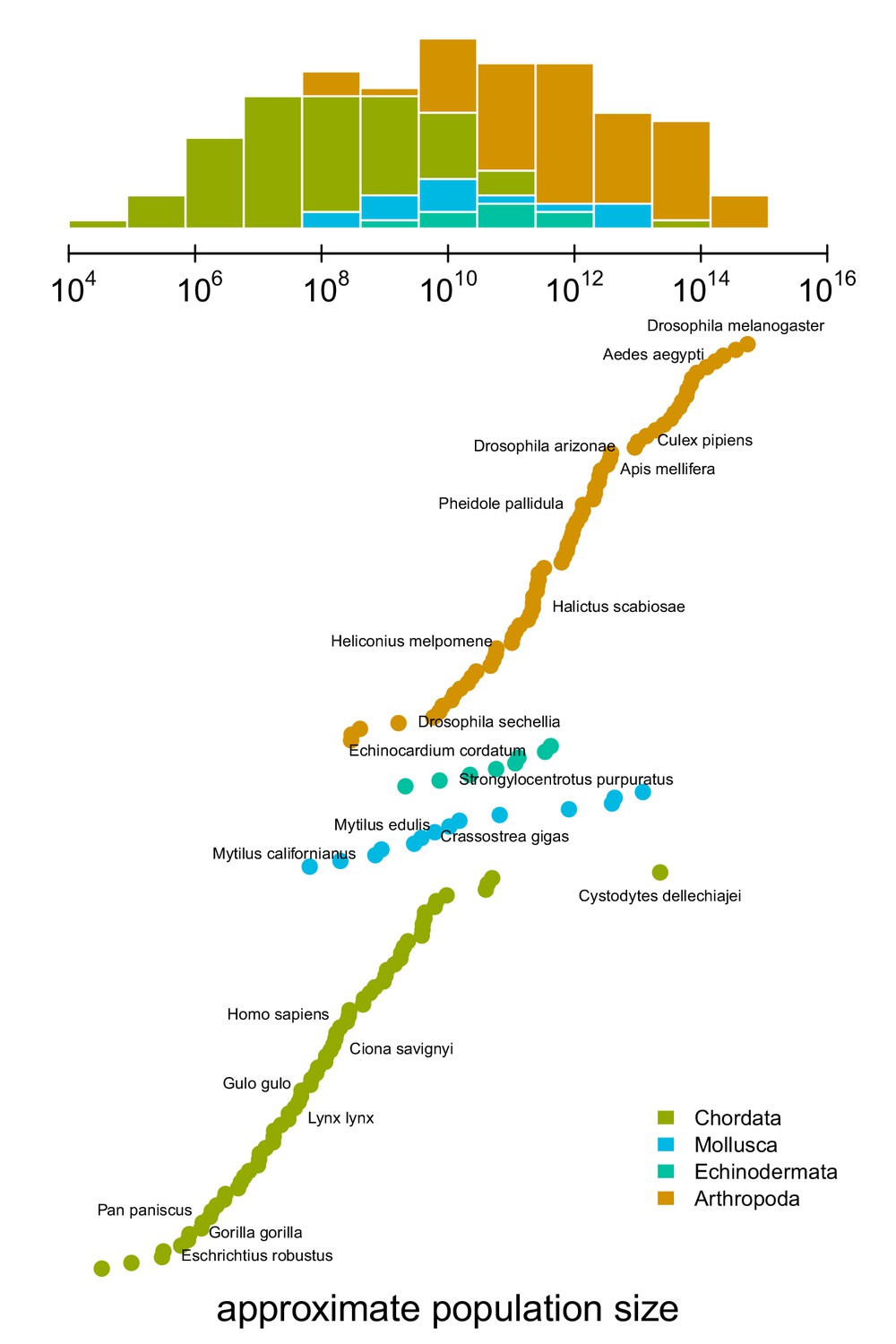
The distribution of approximate census population sizes estimated by this study.

Some phyla containing few species were excluded for clarity.

Figure 1—source data 1 The population size estimates for 172 metazoan taxa.: https://cdn.elifesciences.org/articles/67509/elife-67509-fig1-data1-v3.zip
Download elife-67509-fig1-data1-v3.zip

Figure 1—figure supplement 1

Download asset Open asset

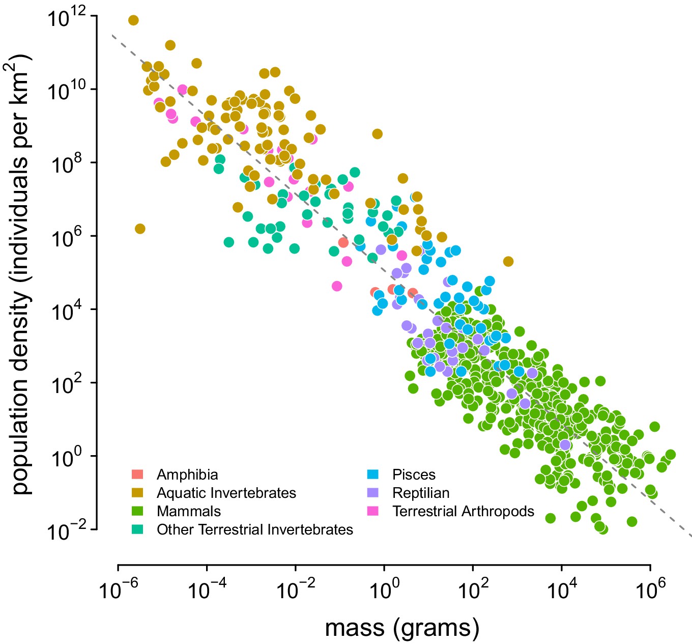
The relationship between body mass and population density found by Damuth, 1987, which is used to predict population densities.

The source of this data is appendix table of Damuth, 1987; the color indicates Damuth’s original group labels. The dashed line was estimated using a lognormal regression model in Stan. References to each measurement are available in Damuth, 1987.

Figure 1—figure supplement 2

Download asset Open asset

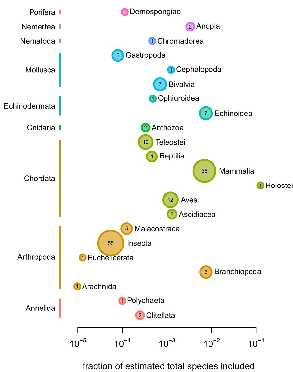
The fraction of total species per class on earth included in this study’s sample, per class.

The color of the points represents phylum, and the size of the point represents the absolute number of species by class.

Figure 1—figure supplement 3

Download asset Open asset

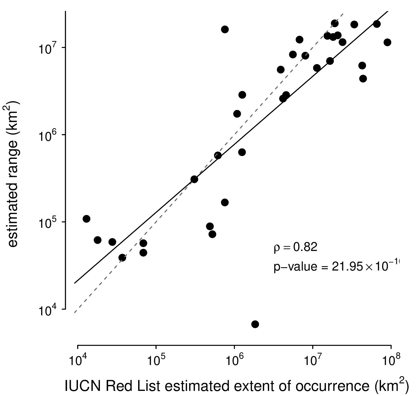
Comparison of this paper’s range estimates procedure against the IUCN Red List’s range estimates.

The correspondence between the ranges estimated with the alpha hull method applied to GBIF data used in this paper and IUCN Red List’s Extent of Occurrence for the subset of species in both datasets. Note that the IUCN Red List contains predominantly endangered species, which leads to ascertainment bias; still, the high correlation between the estimated ranges shows the alpha hull method works well.

Figure 1—figure supplement 4

Download asset Open asset

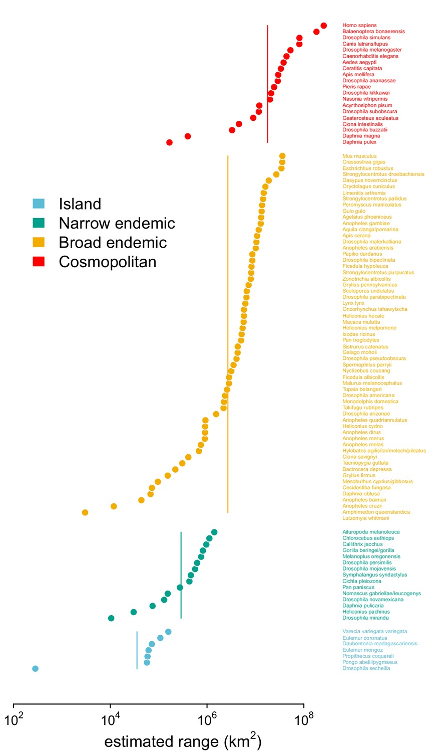
Validation of this paper’s range estimates against the categorical labels of Leffler et al., 2012.

The estimated ranges using GBIF occurrence data, ordered within and colored by the original range category labels assigned in Leffler et al., 2012.

Figure 1—figure supplement 5

Download asset Open asset

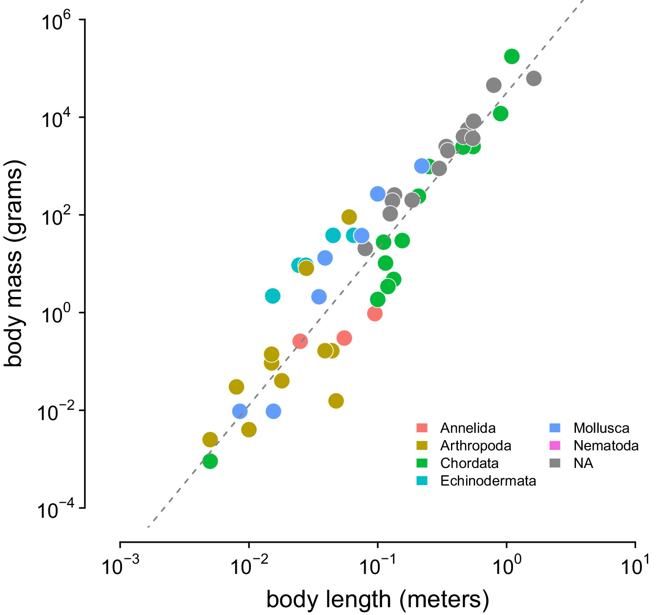
The relationship between body length (meters) and body mass (grams) in the Romiguier et al., 2014 data set.

The relationship between body length (meters) and body mass (grams) in the Romiguier et al., 2014 data set. This is used to infer body masses for taxa. The gray dashed line is the line of best fit inferred using Stan.

Figure 2 with 4 supplements

Download asset Open asset

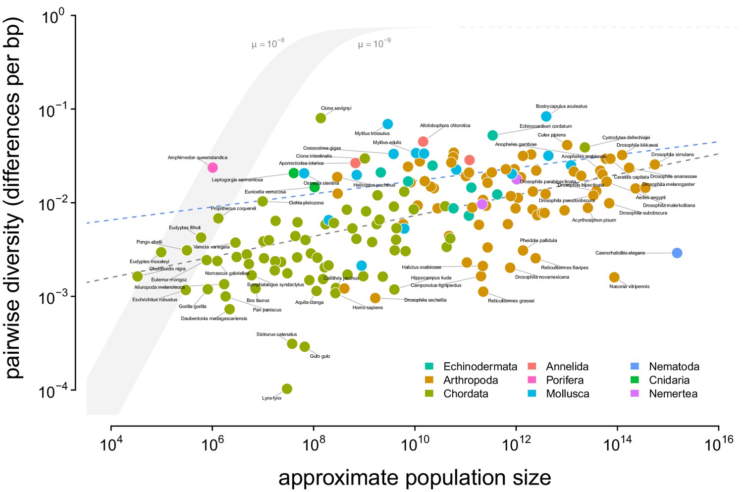
A visualization of Lewontin’s Paradox of Variation.

Pairwise diversity (data from Leffler et al., 2012, Corbett-Detig et al., 2015, and Romiguier et al., 2014), which varies over three orders of magnitude, shows a weak relationship with approximate population size, which varies over 12 orders of magnitude. The shaded curve shows the range of expected neutral diversity if $N_{e}$ were to equal $N_{c}$ under the four-alleles model, $\log_{10} (π) = \log_{10} (θ) - \log_{10} (1 + 4 θ / 3)$ where $θ = 4 N_{c} μ$ , for two mutation rates, $μ = 10^{- 8}$ and $μ = 10^{- 9}$ , and the light gray dashed line represents the maximum pairwise diversity under the four alleles model. The dark gray dashed line is the OLS regression fit, and the blue dashed line is the regression fit using a phylogenetic mixed-effects model. Points are colored by phylum. The species *Equus ferus przewalskii* ( $N_{c} \approx 10^{3}$ and $π = 3.6 \times 10^{- 3}$ ) was an outlier and excluded from this figure for visual clarity.

Figure 2—source data 1 The diversity and population size dataset for 172 metazoan taxa.: https://cdn.elifesciences.org/articles/67509/elife-67509-fig2-data1-v3.zip
Download elife-67509-fig2-data1-v3.zip

Figure 2—figure supplement 1

Download asset Open asset

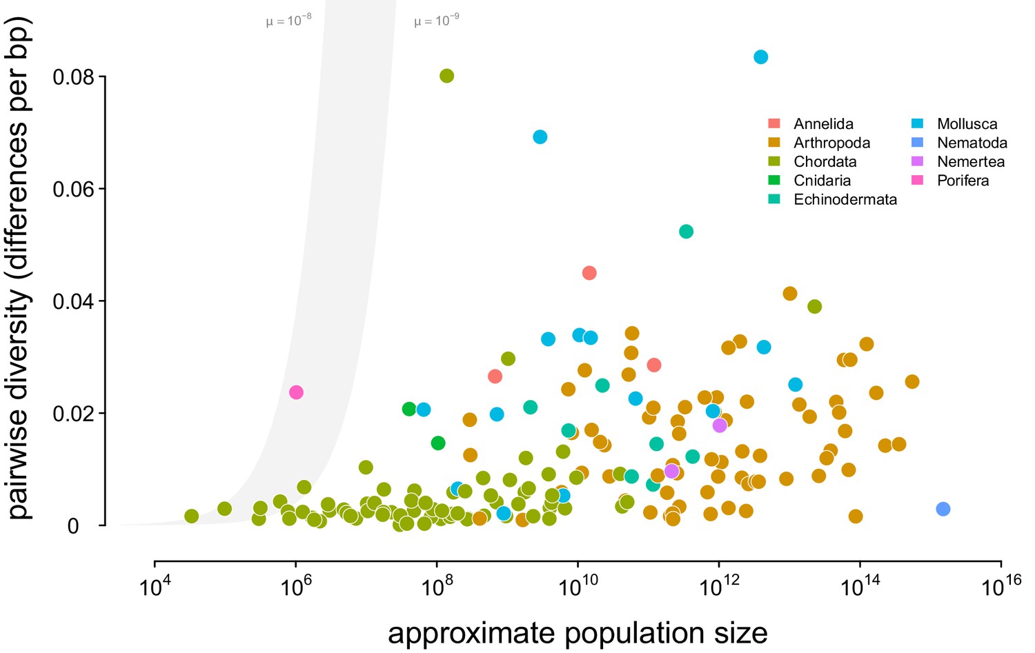
A linear-log version of Figure 2.

Points are colored by phylum, and the shaded region is the predicted neutral level of diversity assuming $N_{e} = N_{c}$ with mutation range ranging between $10^{- 9} \leq μ \leq 10^{- 8}$ .

Figure 2—figure supplement 2

Download asset Open asset

A version of Figure 2 with OLS estimates per phylum.

Diversity and approximate population size for 172 taxa, colored by phylum; the dashed lines indicate the non-phylogenetic OLS estimates of the relationship between population size and diversity grouped by phyla.

Figure 2—figure supplement 3

Download asset Open asset

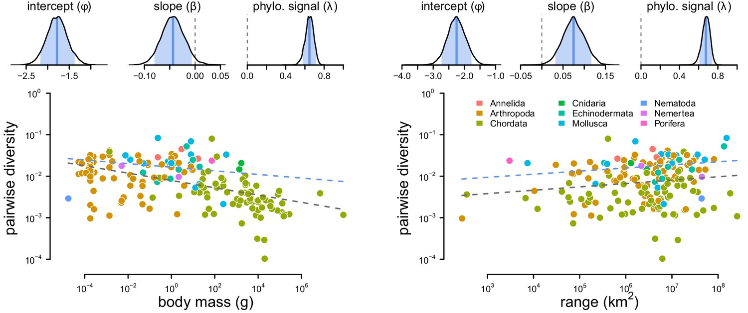
The posterior distributions and fitted relationship between diversity and both body mass and range size.

The relationship between diversity (differences per basepair) and body mass (left) and range (right) across 172 species. The top row are posterior distributions of parameters estimated using the phylogenetic mixed-effects model using 166 taxa in the synthetic phylogeny for the intercept, slope, and phylogenetic signal from the mixed-effects model. The bottom row contain each species as a point, colored by phyla. The gray dashed line is the non-phylogenetic standard regression estimate, and the blue dashed line is the relationship fit by the phylogenetic mixed-effects model.

Figure 2—figure supplement 4

Download asset Open asset

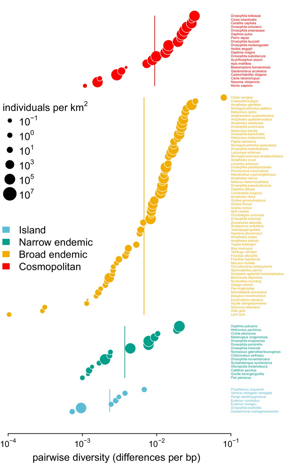
Pairwise diversity grouped by the range categories from Leffler et al., 2012, with point size indicating the predicted population density.

The vertical lines are the range category group means.

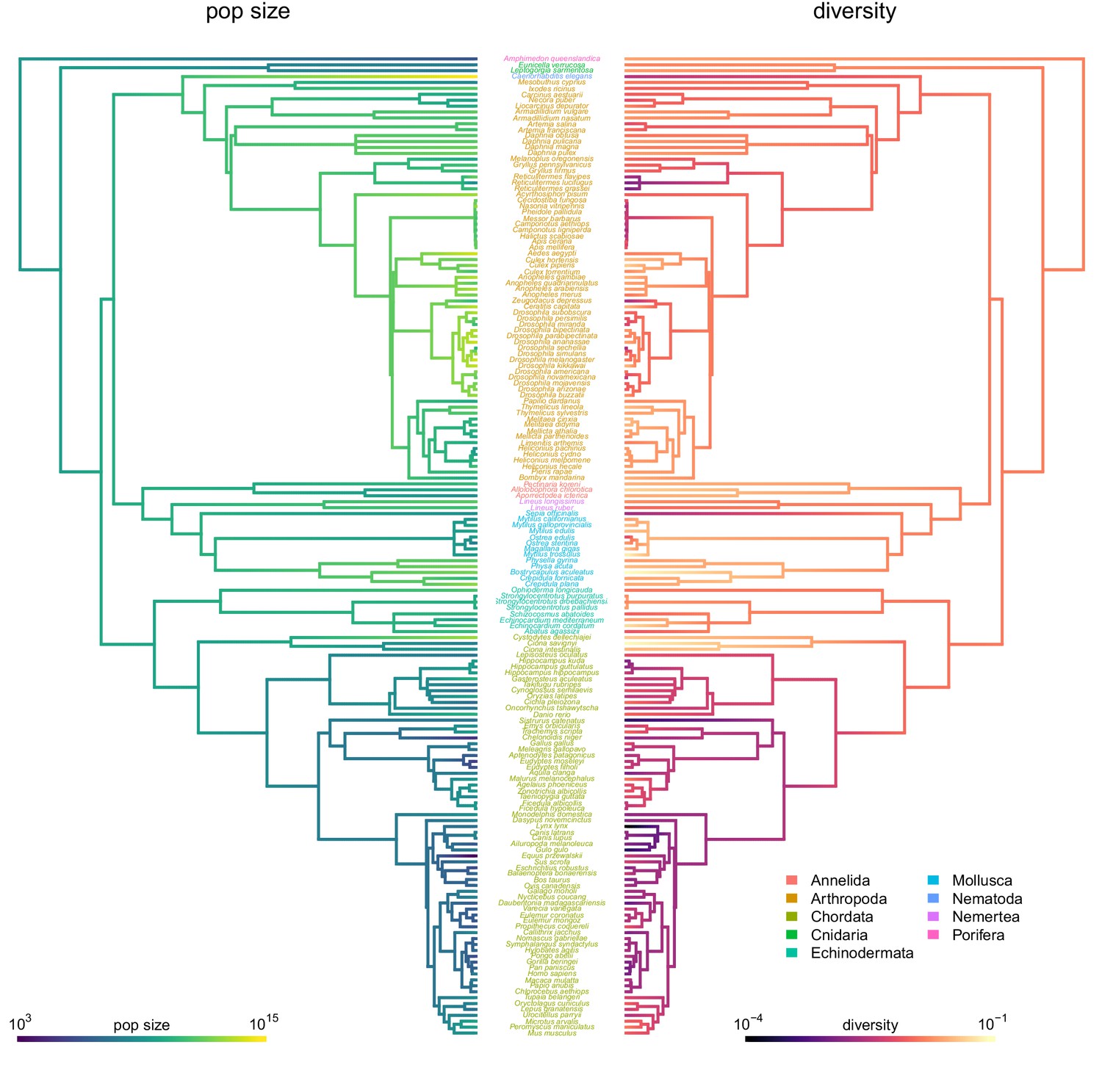
Figure 3 with 3 supplements

Download asset Open asset

Phylogenetic comparative models of diversity and population size.

(A) The ancestral continuous trait estimates for the population size and diversity (differences per bp, log scaled) across the phylogeny of 166 taxa. The phyla of the tips are indicated by the color bar in the center. (B) The posterior distributions of the intercept, slope, and phylogenetic signal (λ, de Villemereuil and Nakagawa, 2014) of the phylogenetic mixed-effects model of diversity and population size (log scaled). Also shown are the 90% credible interval (light blue shading), posterior mean (blue line), OLS estimate (gray solid line), and bootstrap OLS confidence intervals (light gray shading). (C) The node-height tests of diversity, population size, and the two components of the population size estimates, body mass, and range (all traits on log scale before contrast was calculated). Each point shows the standardized phylogenetic independent contrast and branching time for a pair of lineages. Red lines are robust regression estimates (and are only shown for statistically significant relationships at the $α = 0.05$ level). Note that some outlier pairs with very high phylogenetic independent contrasts were excluded (in all cases, these outliers were in the genus *Drosophila*).

Figure 3—figure supplement 1

Download asset Open asset

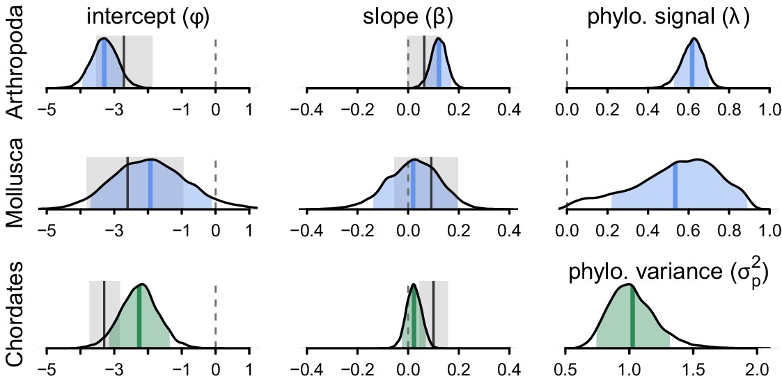
The posterior distributions for the parameters of the phylogenetic mixed-effects model of diversity and population size (this is analogous to Figure 3B) fit separately on chordates ( $n = 68$ ), molluscs ( $n = 13$ ), and arthropods ( $n = 68$ ).

The phylogenetic mixed-effects model for chordates indicated the best-fitting model had no residual variance ( $σ_{r}^{2} = 0$ ), so an alternate model without this variance component was used to ensure proper convergence; this model is shown in green. The light blue (green) shaded regions are the 90% credible intervals, the blue (green) lines the posterior averages, the gray shaded regions the OLS bootstrap 95% confidence intervals, and the gray lines the OLS estimate. Note that unlike Figure 3, the OLS estimate uses all taxa, not just those present in the phylogeny, since splitting the data by phyla reduces sample sizes (OLS with just the subset of taxa in the phylogeny is not significant for either chordates and arthropods). The vertical dashed gray line indicates zero.

Figure 3—figure supplement 2

Download asset Open asset

The ancestral continuous trait estimates for diversity and population size with species labels.

Figure 3—figure supplement 3

Download asset Open asset

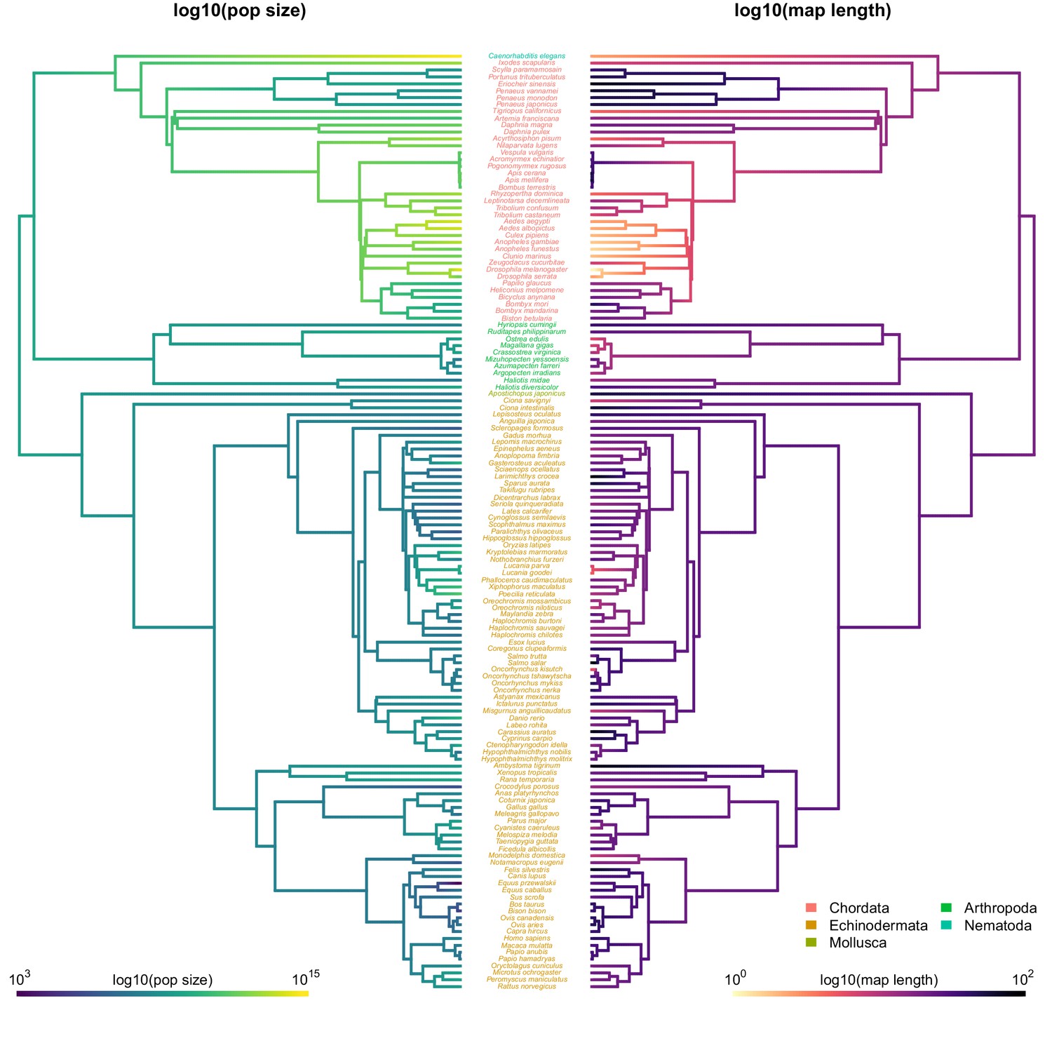
The ancestral continuous trait estimates for recombination map length and diversity and population size with species labels.

Figure 4 with 5 supplements

Download asset Open asset

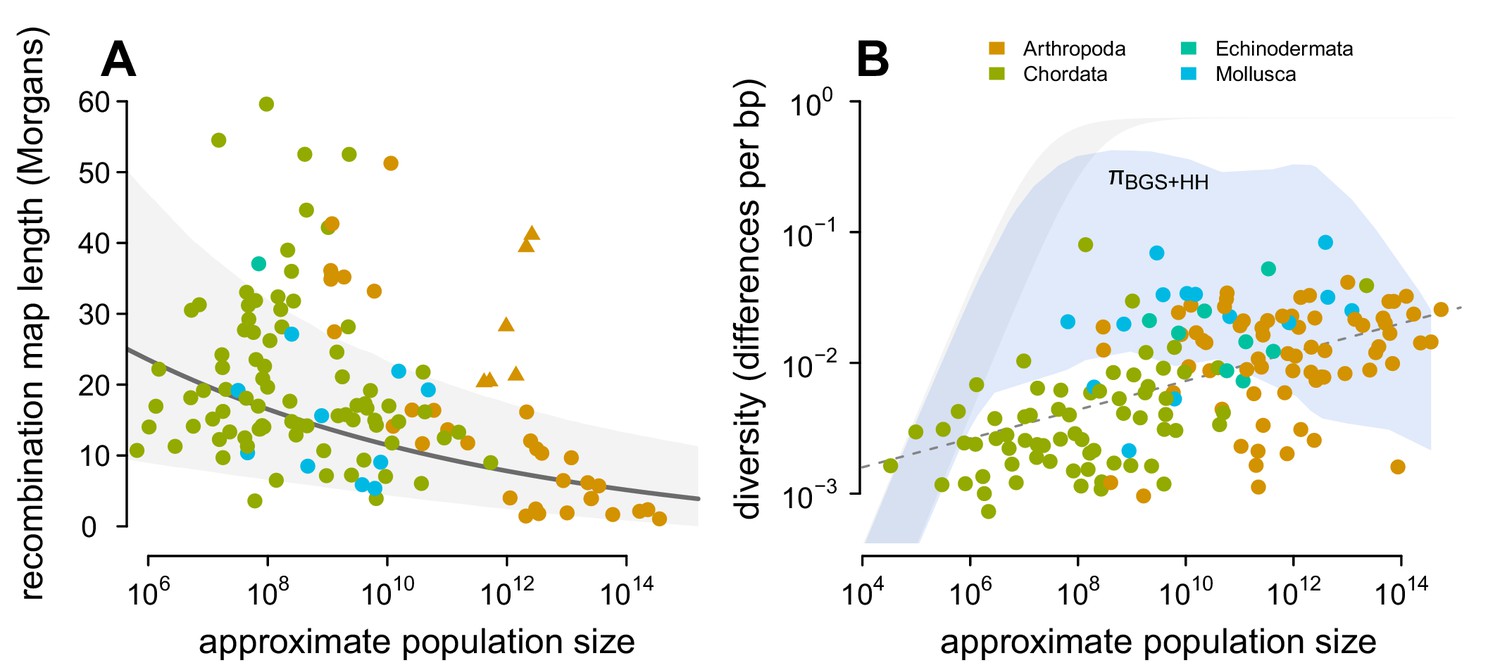
Predicting the impact of linked selection on diversity.

(A) The observed relationship between recombination map length ( $L$ ) and census size ( $N_{c}$ ) across 136 species with complete data and known phylogeny. Triangle points indicate six social taxa excluded from the model fitting since these have adaptively higher recombination map lengths (Wilfert et al., 2007). The dark gray line is the estimated relationship under a phylogenetic mixed-effects model, and the gray interval is the 95% posterior average. (B) Points indicate the observed π– $N_{c}$ relationship across taxa shown in Figure 2, and the blue ribbon is the range of predicted diversity were $N_{e} = N_{c}$ for $μ = 10^{- 8}$ – $10^{- 9}$ , and after accounting for the expected reduction in diversity due to background selection and recurrent hitchhiking under *Drosophila melanogaster* parameters. In both plots, point color indicates phylum.

Figure 4—source data 1 The map length, population size, and linked selection estimates for 136 metazoan taxa.: https://cdn.elifesciences.org/articles/67509/elife-67509-fig4-data1-v3.zip
Download elife-67509-fig4-data1-v3.zip

Figure 4—figure supplement 1

Download asset Open asset

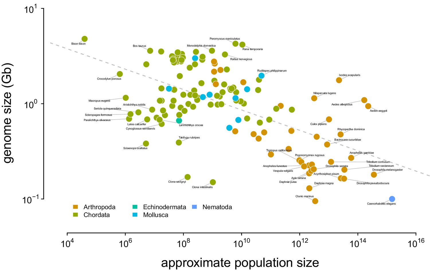
The relationship between genome size and approximate census population size.

The dashed gray line indicates the OLS fit. Tiger salamander (*Ambystoma tigrinum*) was excluded because of its exceptionally large genome size ( 30Gbp).

Figure 4—figure supplement 2

Download asset Open asset

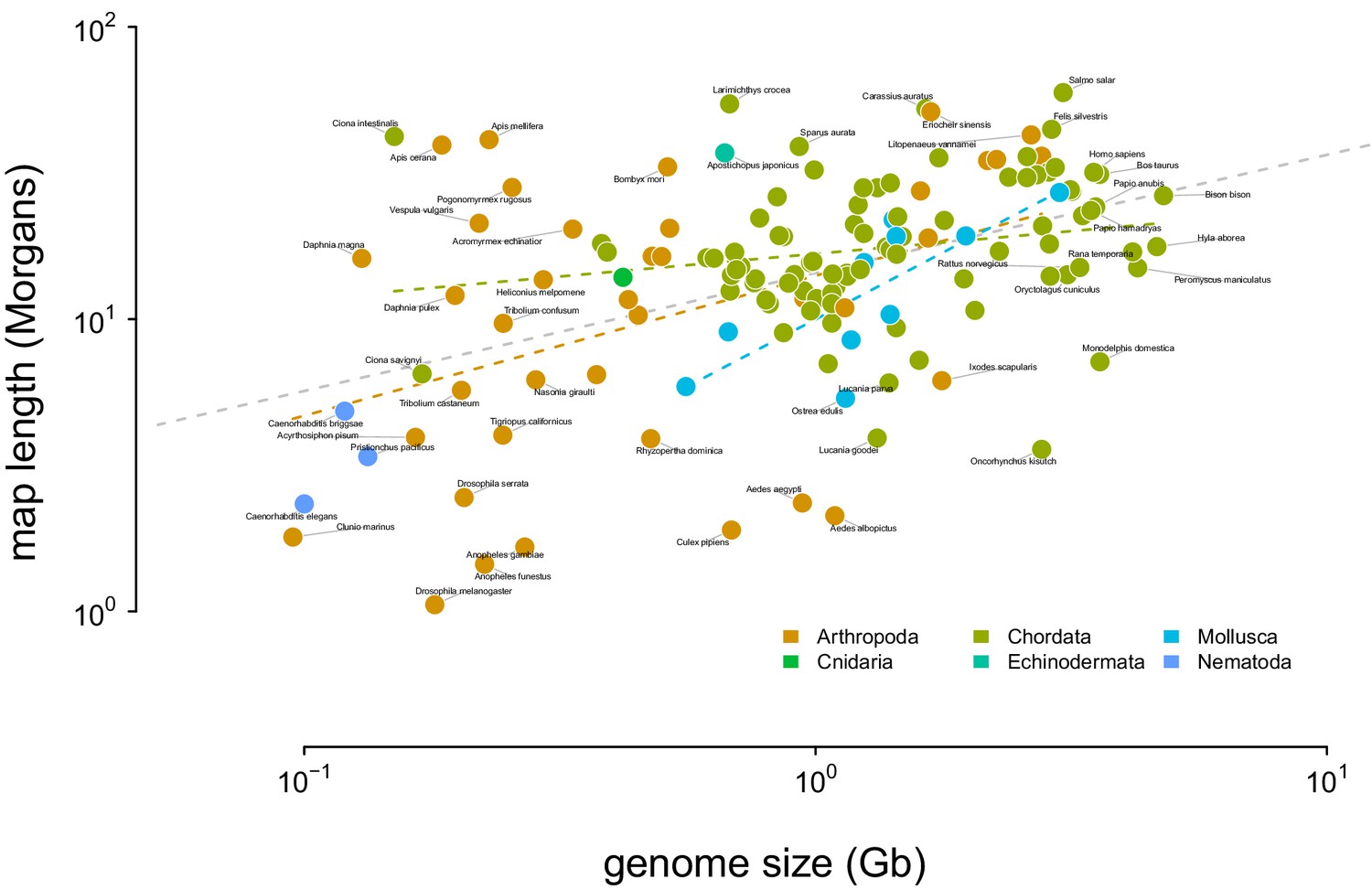
The relationship between genome size and recombination map length.

The dashed gray line indicates the OLS fit for all taxa, and the dashed colored dashed lines indicate the linear relationship fit by phyla. Tiger salamander (*Ambystoma tigrinum*) was excluded because of its exceptionally large genome size ( 30Gbp).

Figure 4—figure supplement 3

Download asset Open asset

The observed π– $N_{c}$ relationship (points) across species compared to the predicted diversity (ribbons) under different modes of linked selection and parameters, for a range of mutation rates, 10^–9–10^–8.

In both subplots, the gray ribbon is the expected diversity if $N_{e} = N_{c}$ . In (A), the predicted impact on diversity for four modes of linked selection are depicted: background selection (purple) and hitchhiking (yellow) individually under the *Drosophila melanogaster* parameters as in Figure 4B, and strong background selection (red) where $U_{strongBGS} = 10 U_{Dmel} \approx 16$ , and strong recurrent hitchhiking, where $γ_{strongHH} = 10 γ_{Dmel} \approx 0.23$ . (B) The predicted diversity under the combined effects of strong background selection and strong hitchhiking (orange) compared to the original predicted diversity as in Figure 4B (blue). Overall, under strong background selection and hitchhiking parameters, predicted diversity would be less than observed for high- $N_{c}$ species, indicating the poor fit to observed data is not sensitive to the choice of *Drosophila melanogaster* parameters.

Figure 4—figure supplement 4

Download asset Open asset

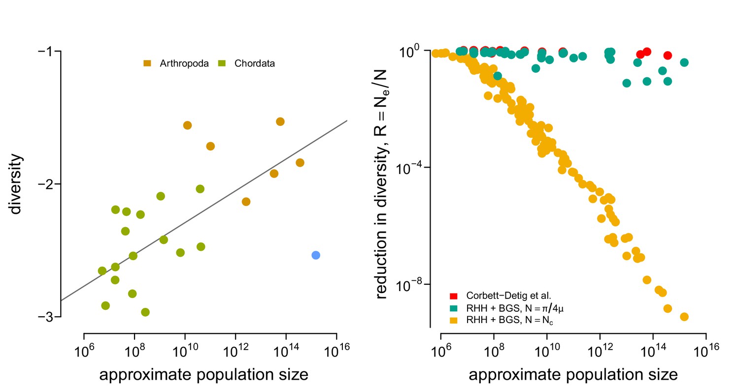
The relationship between $N_{c}$ and diversity in the Corbett-Detig et al., 2015 data, and the relationship between estimated reduction in diversity and census size, for three different approaches.

(A) The diversity data from Corbett-Detig et al., 2015 and the census population size estimated here for metazoan taxa. (B) The reductions in diversity, $R = N_{e} / N$ , plotted against census size across species. The red points are the reductions estimated by Corbett-Detig et al., 2015. This confirms Corbett-Detig et al., 2015 finding that the impact of selection ( $I = 1 - R$ ) increases with census population size (though, in the original paper size body size and range were used as separate proxy variables for census population size). The green and red points are the predicted reduction in diversity under the recurrent hitchhiking (RHH) and background selection (BGS) model using the *Drosophila melanogaster* parameters as described in the main text. The reduction in the diversity due to sweeps, from Equation 1, is determined by the term $2 N S$ . Green points treat $N$ as the implied effective population size from diversity ${\tilde{N}}_{e} = \hat{π} / 4 μ$ , assuming $μ = 10^{- 9}$ . Yellow points treat $N$ as the census size, $N = N_{c}$ . Overall, using the census size, e.g. $2 N_{c} S$ , leads to reductions in diversity that far exceed the empirical estimates of Corbett-Detig et al. and reasonable model-based predictions from ${\tilde{N}}_{e}$ .

Figure 4—figure supplement 5

Download asset Open asset

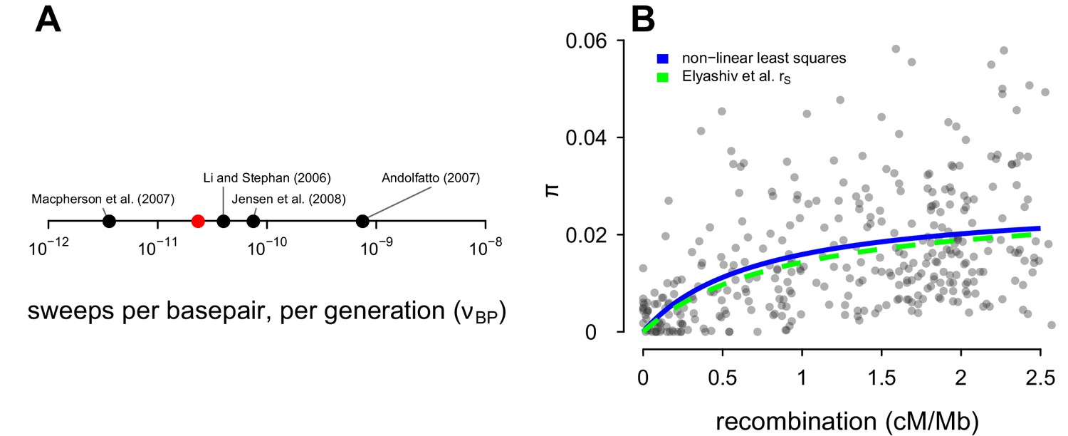
Comparison of the *Drosophila* sweep parameters used in this study with parameters from other studies.

(A) The estimate of the number of sweeps per basepair, per genome ( $ν_{BP}$ ) from Table 2 of Elyashiv et al., 2016 (the studies included are Li and Stephan, 2006; Andolfatto, 2007; Macpherson et al., 2007 and Jensen et al., 2008); the red point is my estimate used in this paper. (B) Points are the data from Shapiro et al., 2007. The blue line is the non-linear least squares fit to the data, and the green dashed line is the sweep model parameterized by the genome-wide average sweep coalescence rate $2 N S \approx 0.92$ from the classic sweep and background selection model of Elyashiv et al., 2016 (r_s in Supplementary Table S6).

Appendix 4—figure 1

Download asset Open asset

A version of Figure 2 with points colored by their IUCN Red List conservation status.

Margin boxplots show the diversity and population size ranges (thin lines) and interquartile ranges (thick lines) for each category. NA/DD indicates no IUCN Red List entry, or Red List status Data Deficient; LC is Least Concern, NT is Near Threatened, VU is Vulnerable, EN is Endangered, and CR is Critically Endangered.

Tables

Table 1

How the total carbon biomass estimates by phylum from Bar-On et al., 2018 compare to the implied biomass estimates from this study.

All biomass estimates are carbon biomass, and the proportions are of total biomass with respect to the study. The proportion of biomass in this study compared to the Bar-On et al. estimates Bar-On et al., 2018 indicates chordates are overrepresented and arthropods are underrepresented in the present study; the factor that each phylum is overrepresented is given in the eighth column. Total species by phylum estimates are from Reaka-Kudla et al., 1996; Nicol, 1969; Zhang, 2013; Chapman, 2009. The ratio column is the ratio of total biomass implied by the $N_{c}$ estimates of each species in a phylum to the actual biomass of that phylum.

		Bar-On et al.		Present study
phylum	total species (T)	biomass (B)	prop. biomass	biomass (b)	prop. biomass	num. species (n)	factor overrepresented	prop. total species (f=n/T)	factor (b/f⁢B)
Arthropoda	1.26 × 10⁶	1.20	0.4635	2.80 × 10⁻⁴	0.0102	68	0.02	5.41 × 10⁻⁵	4.31
Chordata	5.41 × 10⁴	0.87	0.3357	2.67 × 10⁻²	0.9715	68	2.89	1.26 × 10⁻³	24.40
Annelida	1.70 × 10⁴	0.20	0.0772	1.23 × 10⁻⁵	0.0004	3	0.01	1.76 × 10⁻⁴	0.35
Mollusca	9.54 × 10⁴	0.20	0.0772	4.56 × 10^–4	0.0166	13	0.21	1.36 × 10⁻⁴	16.70
Cnidaria	1.60 × 10⁴	0.10	0.0386	3.07 × 10⁻⁵	0.0011	2	0.03	1.25 × 10⁻⁴	2.45
Nematoda	2.50 × 10⁴	0.02	0.0077	4.03 × 10⁻⁶	0.0001	1	0.02	4.00 × 10⁻⁵	5.03

Appendix 4—table 1

The regression estimates of full IUCN Red List population size model for diversity, $\log_{10} (π) = β_{0} + β_{L C} L C + β_{N T} N T + β_{V U} V U + β_{E N} E N + β_{C R} C R + β_{N_{c}} \log_{10} (N_{c})$ ; $d f = 165$ .

Using AIC to compare this full model to a reduced model of $\log_{10} (π) = β_{0} + β_{N_{c}} \log_{10} (N_{c})$ , $A I C_{full} = 204.9$ , $A I C_{reduced} = 216.4$ .

	Mean	2.5 %	97.5 %
$β_{0}$	−2.80	−3.20	−2.50
$β_{L C}$	−0.39	−0.57	−0.21
$β_{N T}$	−0.22	−0.83	0.39
$β_{V U}$	−0.34	−0.84	0.16
$β_{E N}$	−0.40	−0.73	−0.07
$β_{C R}$	−0.03	−0.65	0.59
$β_{N_{c}}$	0.08	0.05	0.11

Additional files

Transparent reporting form: https://cdn.elifesciences.org/articles/67509/elife-67509-transrepform-v3.pdf
Download elife-67509-transrepform-v3.pdf

Download links

A two-part list of links to download the article, or parts of the article, in various formats.

Downloads (link to download the article as PDF)

Open citations (links to open the citations from this article in various online reference manager services)

Mendeley

Cite this article (links to download the citations from this article in formats compatible with various reference manager tools)

Vince Buffalo

(2021)

Quantifying the relationship between genetic diversity and population size suggests natural selection cannot explain Lewontin’s Paradox

eLife 10:e67509.

https://doi.org/10.7554/eLife.67509

Figures

The distribution of approximate census population sizes estimated by this study.

Figure 1—source data 1

The relationship between body mass and population density found by Damuth, 1987, which is used to predict population densities.

The fraction of total species per class on earth included in this study’s sample, per class.

Comparison of this paper’s range estimates procedure against the IUCN Red List’s range estimates.

Validation of this paper’s range estimates against the categorical labels of Leffler et al., 2012.

The relationship between body length (meters) and body mass (grams) in the Romiguier et al., 2014 data set.

A visualization of Lewontin’s Paradox of Variation.

Figure 2—source data 1

A linear-log version of Figure 2.

A version of Figure 2 with OLS estimates per phylum.

The posterior distributions and fitted relationship between diversity and both body mass and range size.

Pairwise diversity grouped by the range categories from Leffler et al., 2012, with point size indicating the predicted population density.

Phylogenetic comparative models of diversity and population size.

The posterior distributions for the parameters of the phylogenetic mixed-effects model of diversity and population size (this is analogous to Figure 3B) fit separately on chordates ( $n = 68$ ), molluscs ( $n = 13$ ), and arthropods ( $n = 68$ ).

The ancestral continuous trait estimates for diversity and population size with species labels.

The ancestral continuous trait estimates for recombination map length and diversity and population size with species labels.

Predicting the impact of linked selection on diversity.

Figure 4—source data 1

The relationship between genome size and approximate census population size.

The relationship between genome size and recombination map length.

The observed π– $N_{c}$ relationship (points) across species compared to the predicted diversity (ribbons) under different modes of linked selection and parameters, for a range of mutation rates, 10^–9–10^–8.

The relationship between $N_{c}$ and diversity in the Corbett-Detig et al., 2015 data, and the relationship between estimated reduction in diversity and census size, for three different approaches.

Comparison of the Drosophila sweep parameters used in this study with parameters from other studies.

A version of Figure 2 with points colored by their IUCN Red List conservation status.

Tables

How the total carbon biomass estimates by phylum from Bar-On et al., 2018 compare to the implied biomass estimates from this study.

The regression estimates of full IUCN Red List population size model for diversity, $\log_{10} (π) = β_{0} + β_{L C} L C + β_{N T} N T + β_{V U} V U + β_{E N} E N + β_{C R} C R + β_{N_{c}} \log_{10} (N_{c})$ ; $d f = 165$ .

Additional files

Transparent reporting form

Download links

Downloads (link to download the article as PDF)

Open citations (links to open the citations from this article in various online reference manager services)

Cite this article (links to download the citations from this article in formats compatible with various reference manager tools)

Be the first to read new articles from eLife

Share this article

Cite this article

The distribution of approximate census population sizes estimated by this study.

Figure 1—source data 1

The relationship between body mass and population density found by Damuth, 1987, which is used to predict population densities.

The fraction of total species per class on earth included in this study’s sample, per class.

Comparison of this paper’s range estimates procedure against the IUCN Red List’s range estimates.

Validation of this paper’s range estimates against the categorical labels of Leffler et al., 2012.

The relationship between body length (meters) and body mass (grams) in the Romiguier et al., 2014 data set.

A visualization of Lewontin’s Paradox of Variation.

Figure 2—source data 1

A linear-log version of Figure 2.

A version of Figure 2 with OLS estimates per phylum.

The posterior distributions and fitted relationship between diversity and both body mass and range size.

Pairwise diversity grouped by the range categories from Leffler et al., 2012, with point size indicating the predicted population density.

Phylogenetic comparative models of diversity and population size.

The posterior distributions for the parameters of the phylogenetic mixed-effects model of diversity and population size (this is analogous to Figure 3B) fit separately on chordates (n=68), molluscs (n=13), and arthropods (n=68).

The ancestral continuous trait estimates for diversity and population size with species labels.

The ancestral continuous trait estimates for recombination map length and diversity and population size with species labels.

Predicting the impact of linked selection on diversity.

Figure 4—source data 1

The relationship between genome size and approximate census population size.

The relationship between genome size and recombination map length.

The observed π–Nc relationship (points) across species compared to the predicted diversity (ribbons) under different modes of linked selection and parameters, for a range of mutation rates, 10–9–10–8.

The relationship between Nc and diversity in the Corbett-Detig et al., 2015 data, and the relationship between estimated reduction in diversity and census size, for three different approaches.

Comparison of the Drosophila sweep parameters used in this study with parameters from other studies.

A version of Figure 2 with points colored by their IUCN Red List conservation status.

How the total carbon biomass estimates by phylum from Bar-On et al., 2018 compare to the implied biomass estimates from this study.

The regression estimates of full IUCN Red List population size model for diversity, log10⁡(π)=β0+βLCLC+βNTNT+βVUVU+βENEN+βCRCR+βNclog10⁡(Nc); df=165.

Transparent reporting form

Downloads (link to download the article as PDF)

Open citations (links to open the citations from this article in various online reference manager services)

Cite this article (links to download the citations from this article in formats compatible with various reference manager tools)

The posterior distributions for the parameters of the phylogenetic mixed-effects model of diversity and population size (this is analogous to Figure 3B) fit separately on chordates ( $n = 68$ ), molluscs ( $n = 13$ ), and arthropods ( $n = 68$ ).

The observed π– $N_{c}$ relationship (points) across species compared to the predicted diversity (ribbons) under different modes of linked selection and parameters, for a range of mutation rates, 10^–9–10^–8.

The relationship between $N_{c}$ and diversity in the Corbett-Detig et al., 2015 data, and the relationship between estimated reduction in diversity and census size, for three different approaches.

The regression estimates of full IUCN Red List population size model for diversity, $\log_{10} (π) = β_{0} + β_{L C} L C + β_{N T} N T + β_{V U} V U + β_{E N} E N + β_{C R} C R + β_{N_{c}} \log_{10} (N_{c})$ ; $d f = 165$ .