Local adaptation and archaic introgression shape global diversity at human structural variant loci
- Department of Biology, Johns Hopkins University, Baltimore, United States
- Department of Computer Science, Johns Hopkins University, United States
Figures
Figure 1 with 7 supplements

Variant graph genotyping of SVs with Paragraph.
(A) Genotyping of SVs was performed using a graph-based approach that represents the reference and alternative alleles of known SVs as edges. The SVs used for graph construction were originally identified from long-read sequencing of 15 individuals (Audano et al., 2019). (B) At candidate SV loci, samples sequenced with short reads are aligned to the graph along the path of best fit, and individuals are genotyped as heterozygous (middle), homozygous for the reference allele (right), or homozygous for the alternative allele (not depicted). We applied this method to the 1KGP dataset to generate population-scale SV genotypes. (C) Allele frequency spectra of SVs genotyped with Paragraph. The left-most bin represents SVs where the alternative allele is absent from the 1KGP sample (AF = 0). Samples are stratified by their 1KGP superpopulation.
-
Figure 1—source data 1
Superpopulation-level allele frequencies of structural variants used to construct allele frequency spectra in Figure 1C.
The third column (‘sum_AC’) provides allele counts, the fourth column (‘sum_NCHROBS’) provides the number of genotyped chromosomes, and the fifth column (‘AF’) provides the alternative allele frequency.
- https://cdn.elifesciences.org/articles/67615/elife-67615-fig1-data1-v3.txt
Figure 1—figure supplement 1
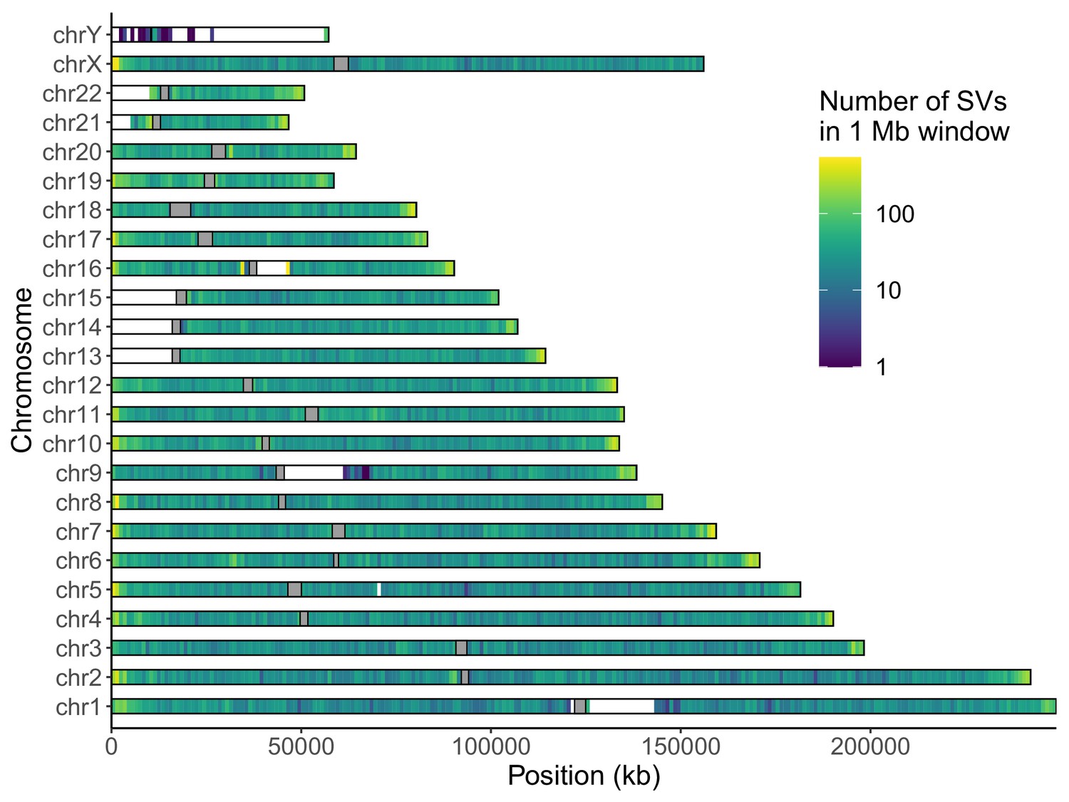
Distribution of long-read discovered SVs throughout the genome.
Coloring indicates the number of SVs in each non-overlapping 1 Mb window. Gray rectangles represent centromeres.
Figure 1—figure supplement 2
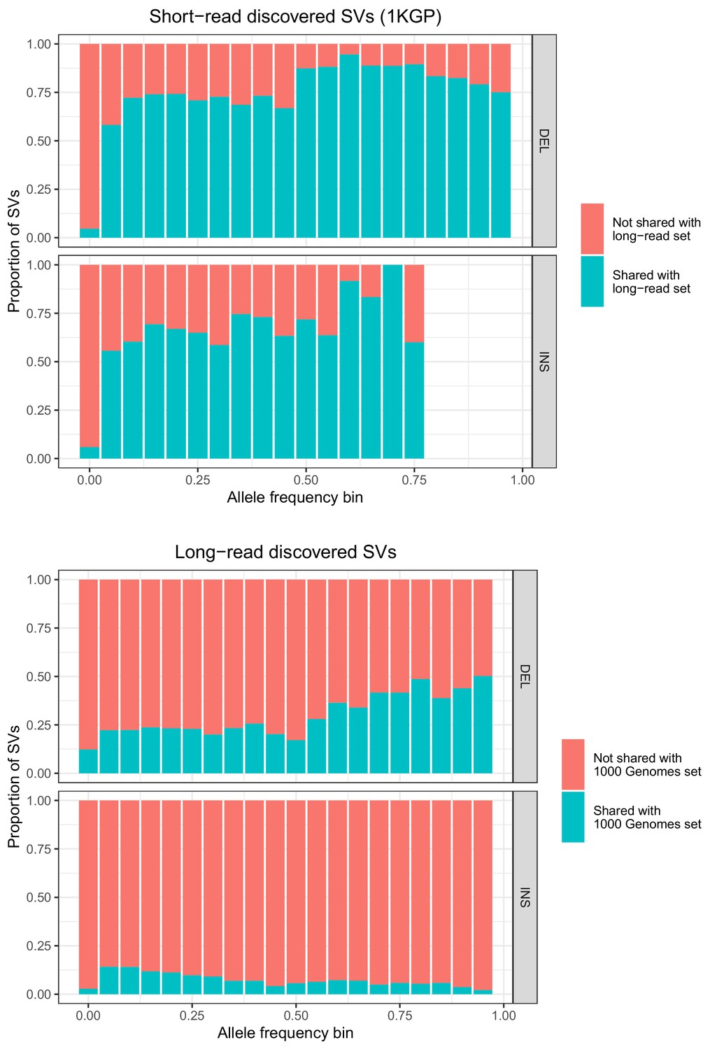
Allele frequencies (AFs) of SVs discovered in 2504 short-read sequenced samples from 1KGP and in 15 long-read sequenced individuals.
SVs are grouped by SV type (deletion, insertion) and then by allele frequency. AFs of the long-read discovered SVs are calculated from their genotypes in 1KGP.
Figure 1—figure supplement 3
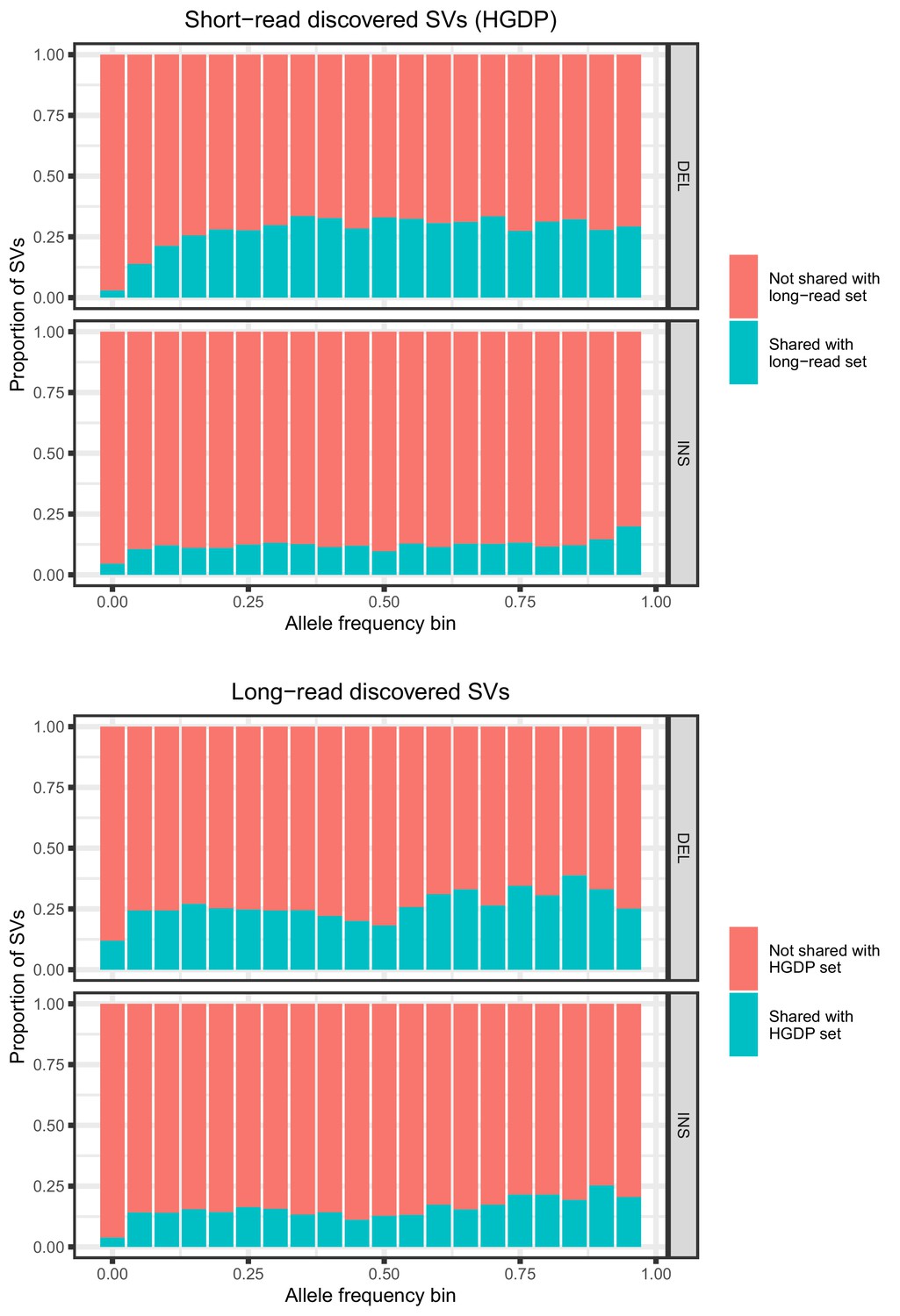
Allele frequencies (AFs) of SVs discovered in 929 short-read sequenced samples from the Human Genome Diversity Project (HGDP) and in 15 long-read sequenced individuals.
SVs are grouped by SV type (deletion, insertion) and then by allele frequency. AFs of the long-read discovered SVs are calculated from their genotypes in 1KGP.
Figure 1—figure supplement 4
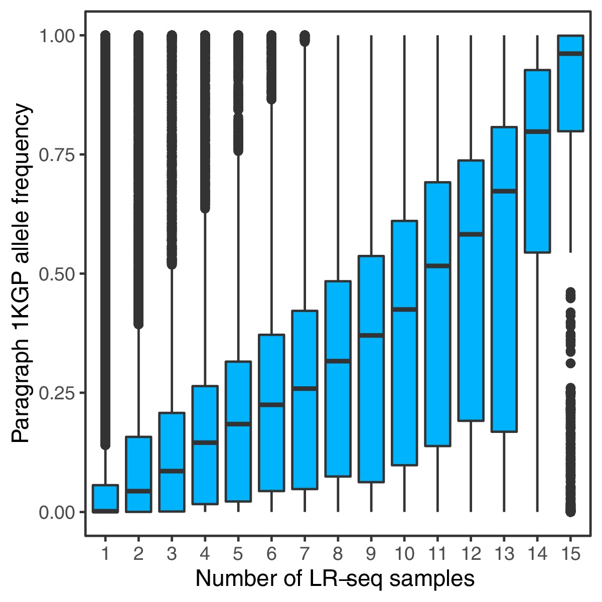
Allele frequencies of SVs genotyped with Paragraph in short-read sequenced samples from 1KGP, compared to the number of PacBio long-read sequenced samples in which the SVs were originally discovered (Audano et al., 2019).
Figure 1—figure supplement 5
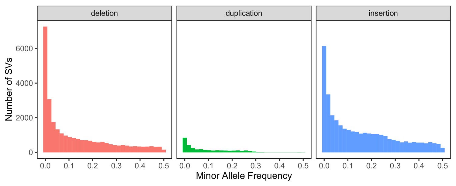
Global minor allele frequency spectrum, stratified by SV type.
Variants with a frequency of 0 are excluded from the histograms for consistency with the comparison in the main text regarding segregating variation.
Figure 1—figure supplement 6
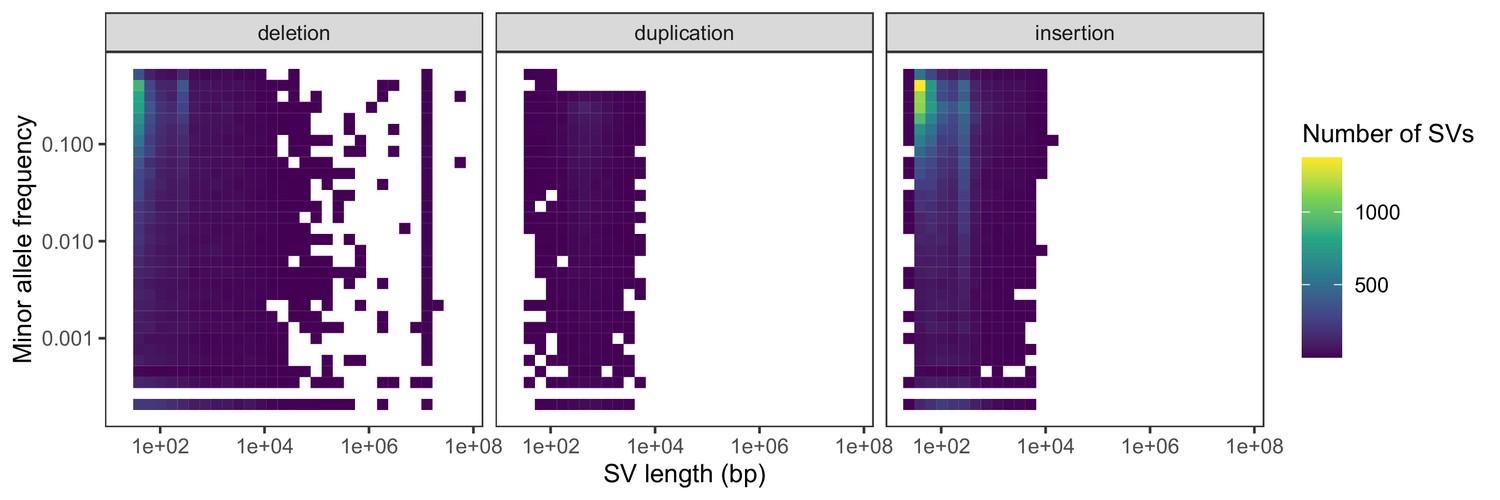
Negative relationships between SV length and global minor allele frequency, stratified by SV type.
Variants with a frequency of 0 are excluded from the heatmaps for consistency with the comparison in the main text regarding segregating variation.
Figure 1—figure supplement 7
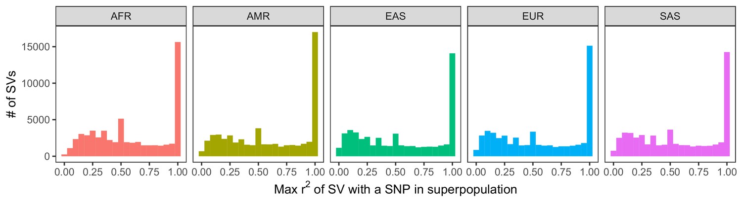
Histogram of LD between SVs and neighboring SNPs and short indels.
LD was calculated within each of the 26 populations of 1KGP. We then determined the maximum LD of every SV with any of the nearest 100 variants, stratifying by superpopulation. The observed peaks at ~0.5, ~0.33, ~0.25, etc. are caused by the mathematical properties of r2, which has maximum values that depend on the allele frequencies of each variant in the tested pair (VanLiere and Rosenberg, 2008; see Materials and methods).
Figure 2 with 2 supplements
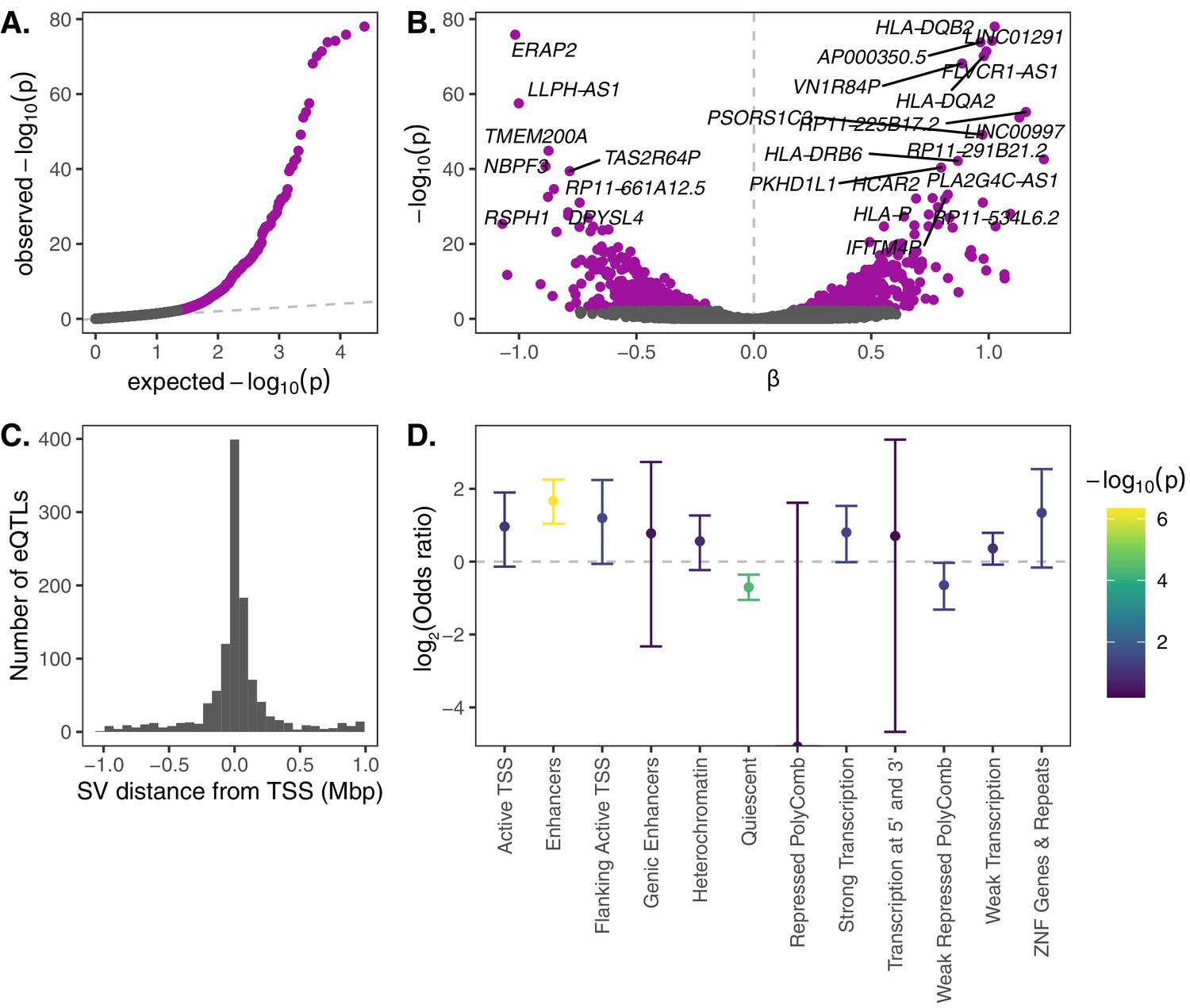
eQTL mapping of SVs.
We used RNA-seq data from the Geuvadis Consortium (Lappalainen et al., 2013), obtained from LCLs derived from individuals from four European and one African population of the 1KGP dataset, to test for associations between SV genotypes and gene expression. SV-eQTL pairs that were significant at a 10% FDR are depicted in purple. (A) Q–Q plot of permutation p-values for all SV-gene pairs tested. (B) Volcano plot of eQTLs and the estimated effect of the alternative allele on expression (β). (C) Distribution of the distance of significant SV eQTLs from the transcription start site (TSS) of their associated genes. (D) Enrichment or depletion of expression associations for SVs that overlap various ChromHMM chromatin state annotations from the Roadmap Epigenomics Project (GM12878 Lymphoblastoid Cells). Chromatin states with ≤0.1% genome-wide representation were omitted for visual clarity.
-
Figure 2—source data 1
Summarized eQTL data underlying Figure 2.
SV IDs, gene IDs and names, distance to the TSS, slopes, p-values, and q-values are provided.
- https://cdn.elifesciences.org/articles/67615/elife-67615-fig2-data1-v3.txt
Figure 2—figure supplement 1
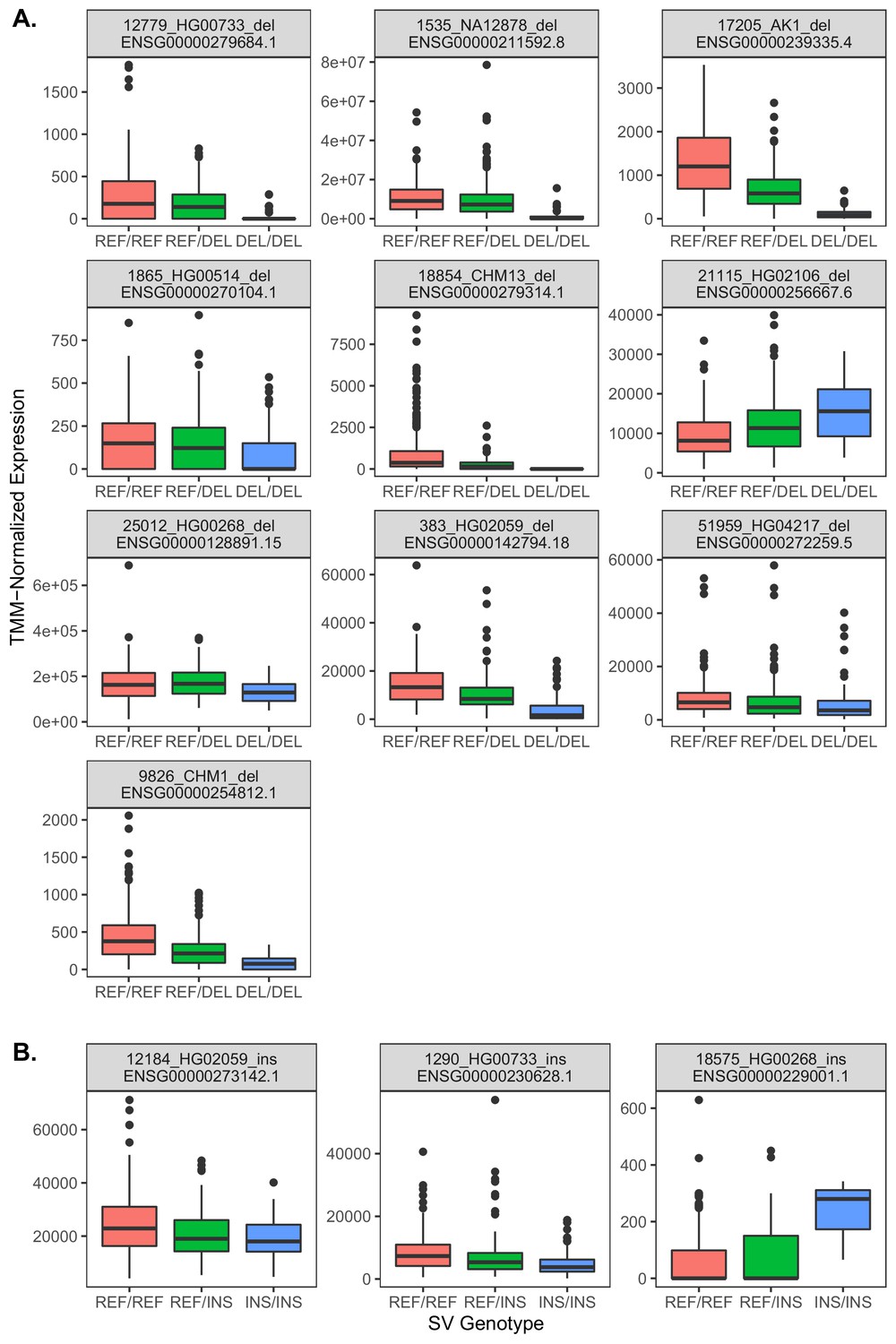
Relationships between gene expression and genotype for 13 exon-intersecting SV eQTLs.
(A) Results for deletions, which in eight of nine cases exhibit negative relationships with expression, consistent with direct dosage effects. (B) Results for insertions, which in two cases exhibit negative relationships, but one case exhibits a positive relationship.
Figure 2—figure supplement 2
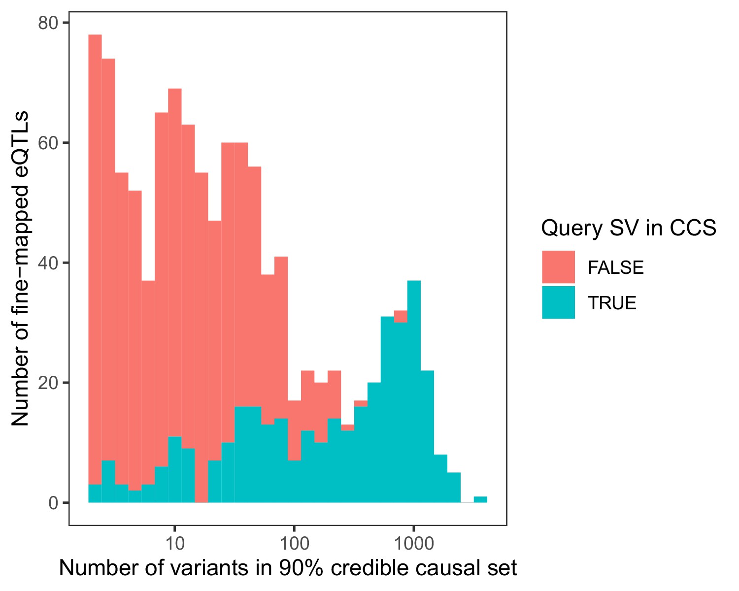
Stacked histogram of the number of variants in each 90% credible causal set based on fine-mapping of 1121 significant SV eQTLs with CAVIAR (Hormozdiari et al., 2014).
Loci are colored based on whether the originally associated SV itself occurred within the 90% credible causal set (CCS).
Figure 3 with 3 supplements
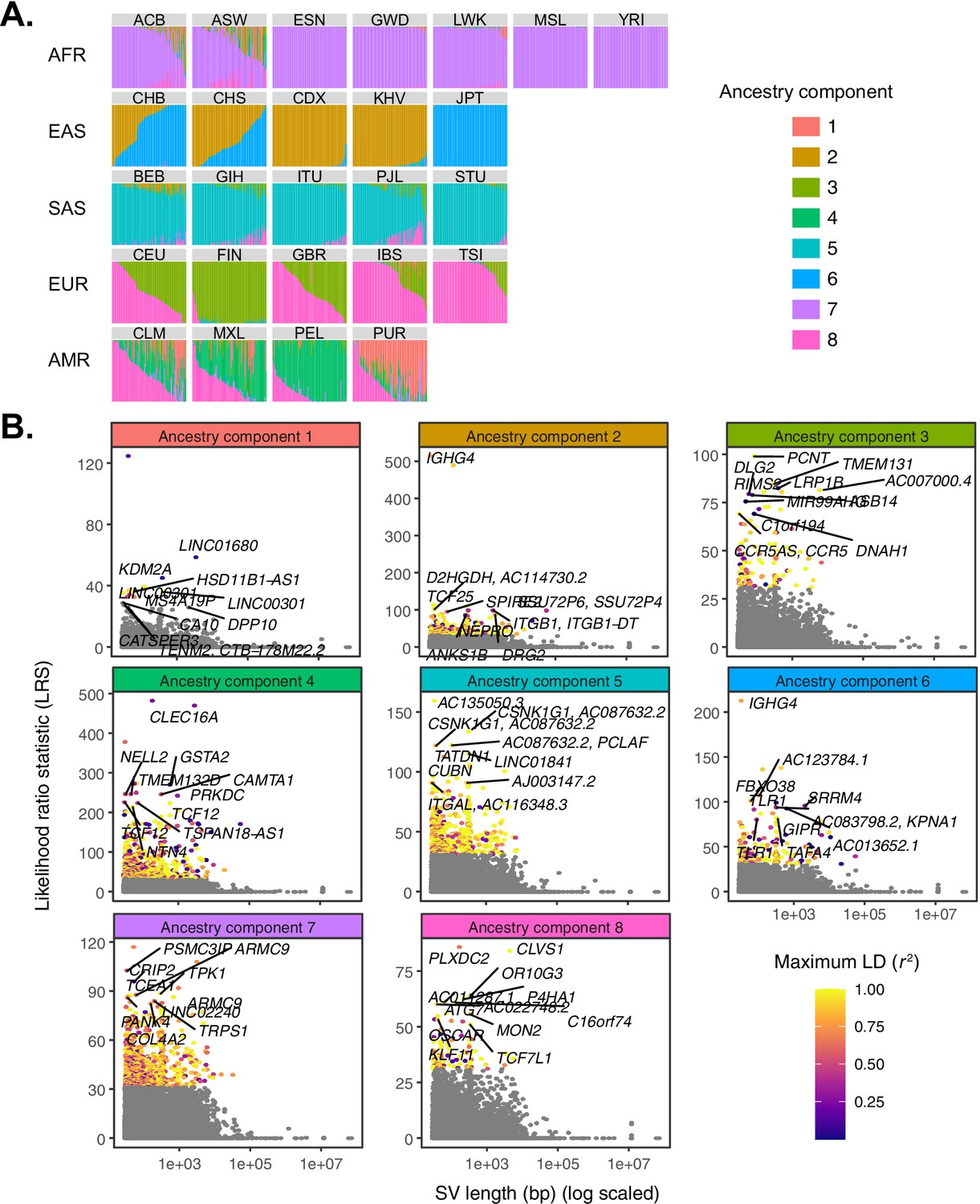
Quantifying allele frequency differentiation among ancestry components.
(A) To conduct an admixture-aware scan for local adaptation, we used Ohana (Cheng et al., 2017; Ilardo et al., 2018) to infer genome-wide patterns of ancestry in the 1KGP samples. This method models each individual as a combination of k ancestry components and then searches for evidence of local adaptation on these component lineages. Admixture proportions (k = 8) for all samples in the 1KGP dataset, grouped by population. Vertical bars represent individual genomes. (B) Using Ohana, we searched for evidence of local adaptation by testing whether the allele frequencies of individual variants were better explained by the genome-wide covariance matrix, or by an alternative covariance matrix where allele frequencies were allowed to vary in one ancestry component. The likelihood ratio statistic (LRS) reflects the relative support for the latter selection hypothesis. For each ancestry component, SVs with LRS > 32 are colored by their maximum linkage disequilibrium (r2) with any known SNP in the corresponding 1KGP superpopulation.
-
Figure 3—source data 1
Ancestry component results underlying Figure 3A.
Ancestry proportions for each individual are provided, along with that individual’s 1KGP population code.
- https://cdn.elifesciences.org/articles/67615/elife-67615-fig3-data1-v3.txt
Figure 3—figure supplement 1
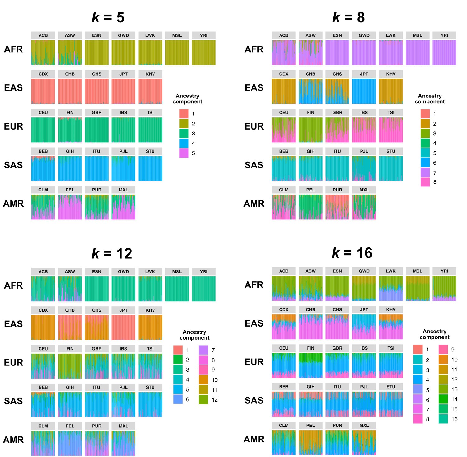
Comparison of admixture proportions inferred by Ohana for samples in the 1KGP dataset.
Admixture was inferred with k = 5, 8 (used in our study), 10, and 16 ancestry components. Vertical bars represent individual samples and are grouped by population.
Figure 3—figure supplement 2
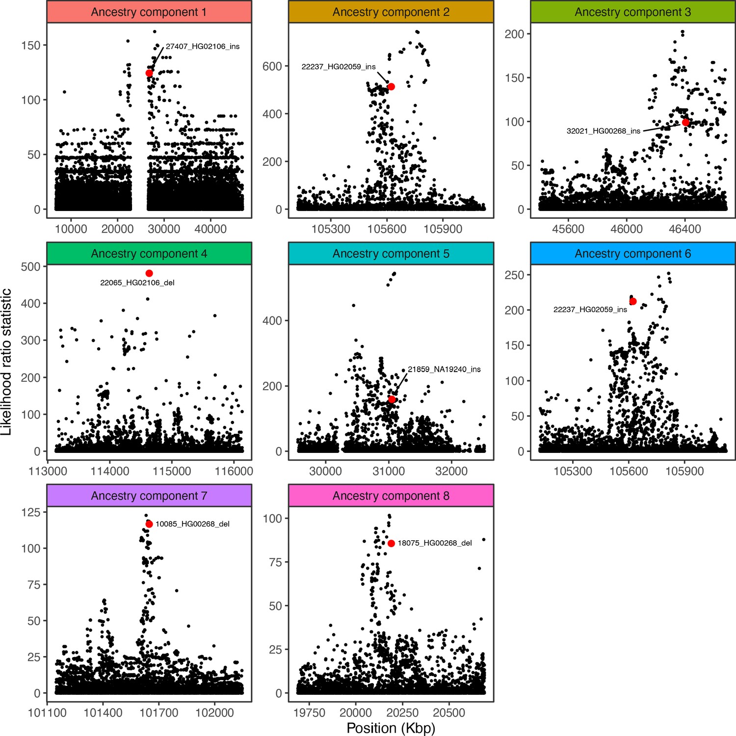
Visualization of the likelihood ratio statistic for SNPs and short indels in the genomic vicinity of the top SV hit for each ancestry component.
SNPs and short indels are colored in black, while SVs are indicated with red.
Figure 3—figure supplement 3
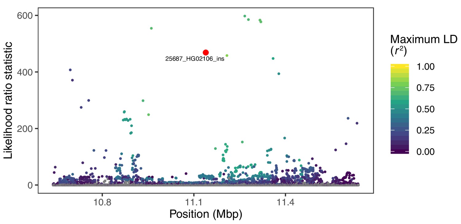
Visualization of the likelihood ratio statistic for SNPs and short indels in the genomic vicinity of a 2.8 kb insertion in the gene CLEC16A.
This SV reaches high allele frequencies in ancestry component 4, corresponding to the Peruvian (PEL), Mexican (MXL), and Colombian (CLM) populations of 1KGP. SNPs and short indels are colored based on their maximum pairwise LD with the target SV among the PEL, MXL, and CLM populations, while the target SV itself is indicated with red.
Figure 4 with 8 supplements
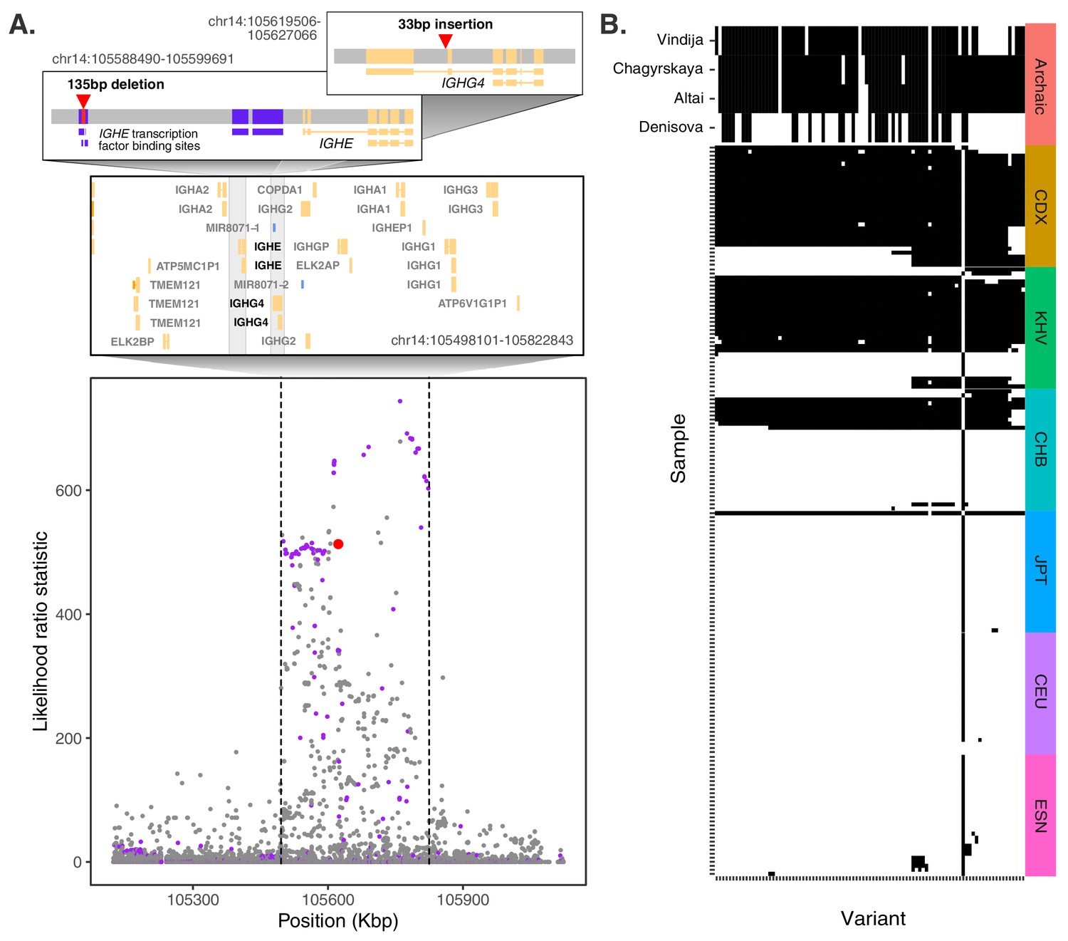
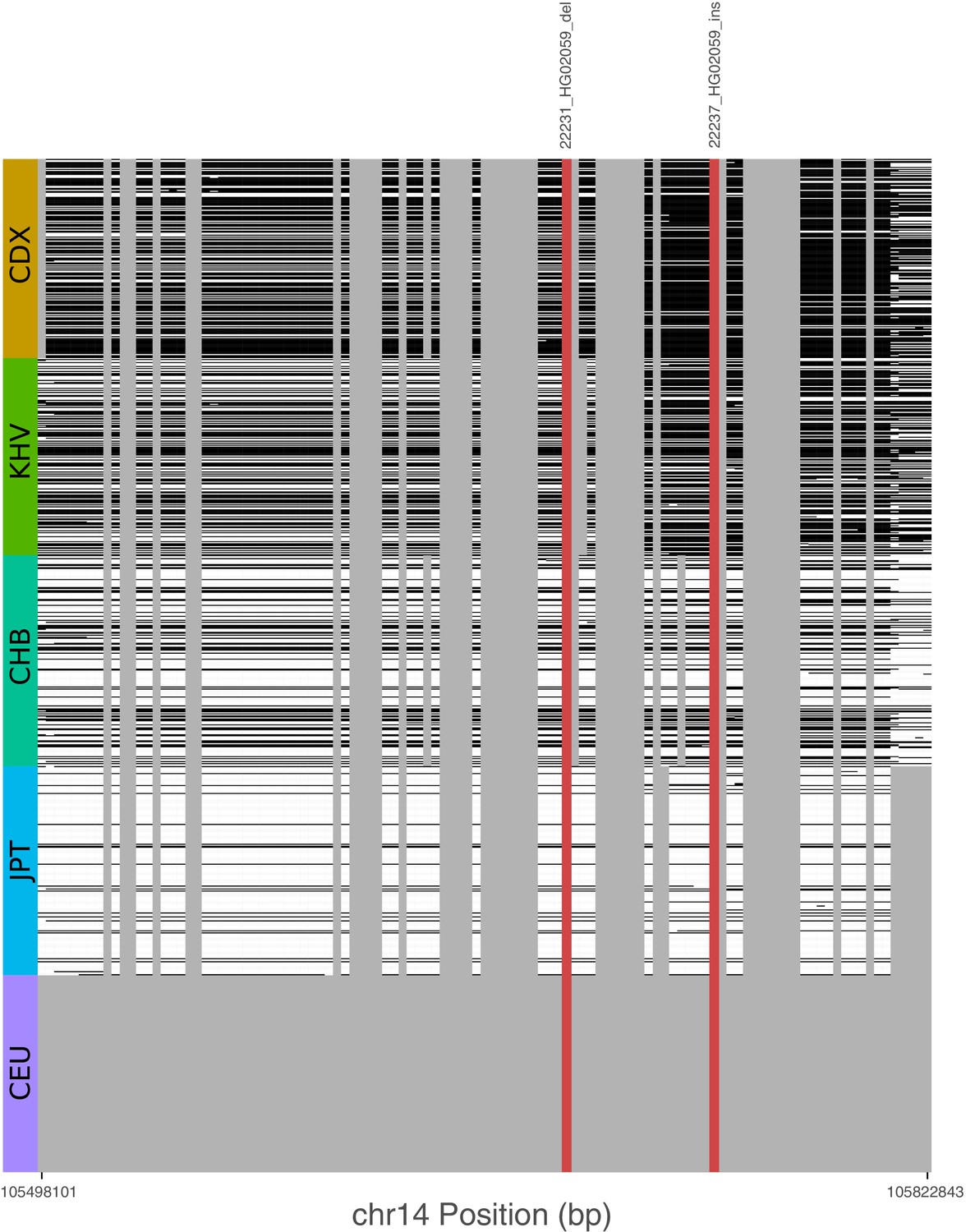
Evidence for Neanderthal introgression of the adaptive IGH haplotype.
(A) Local analysis of likelihood ratio statistics (LRS) in the region near the 33 bp insertion (red point) reveals a 325 kb haplotype encompassing 94 SNPs with strong allele frequency differentiation within ancestry component 2. Points where the alternative allele matches an allele observed in the Chagryskaya Neanderthal genome but at a frequency of 1% or less in African populations are highlighted in purple. (B) Individual haplotypes defined by the highly differentiated SNPs (LRS > 450). Four archaic hominin genomes are plotted at the top, while 30 randomly sampled haplotypes from each of 6 populations from 1KGP are plotted below. Archaic hominins samples are colored according to whether they possess more than one aligned read supporting the alternative allele at a given site. ESN refers to the Esan in Nigeria population of 1KGP. Other 1KGP population codes are provided in the main text.
Figure 4—figure supplement 1
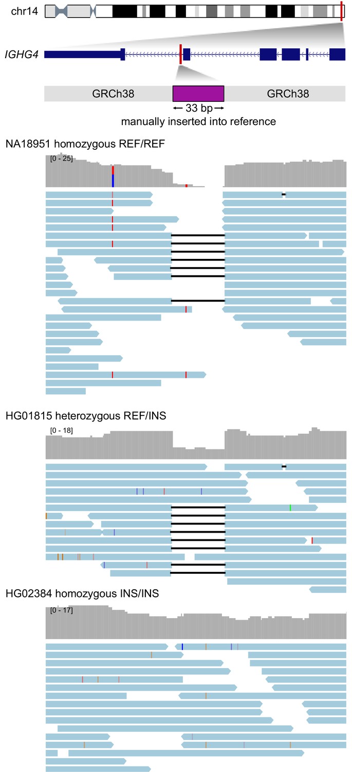
Visualization of read alignments to a modified version of the reference genome at the IGHG4 locus including the intronic 33 bp insertion sequence.
Three samples are depicted as representative of each genotype class (homozygous reference, heterozygous, homozygous alternative). Depth of coverage is plotted in upper tracks, while corresponding read alignments are plotted below. Soft-clipped portions of reads were removed to assist visualization.
Figure 4—figure supplement 2
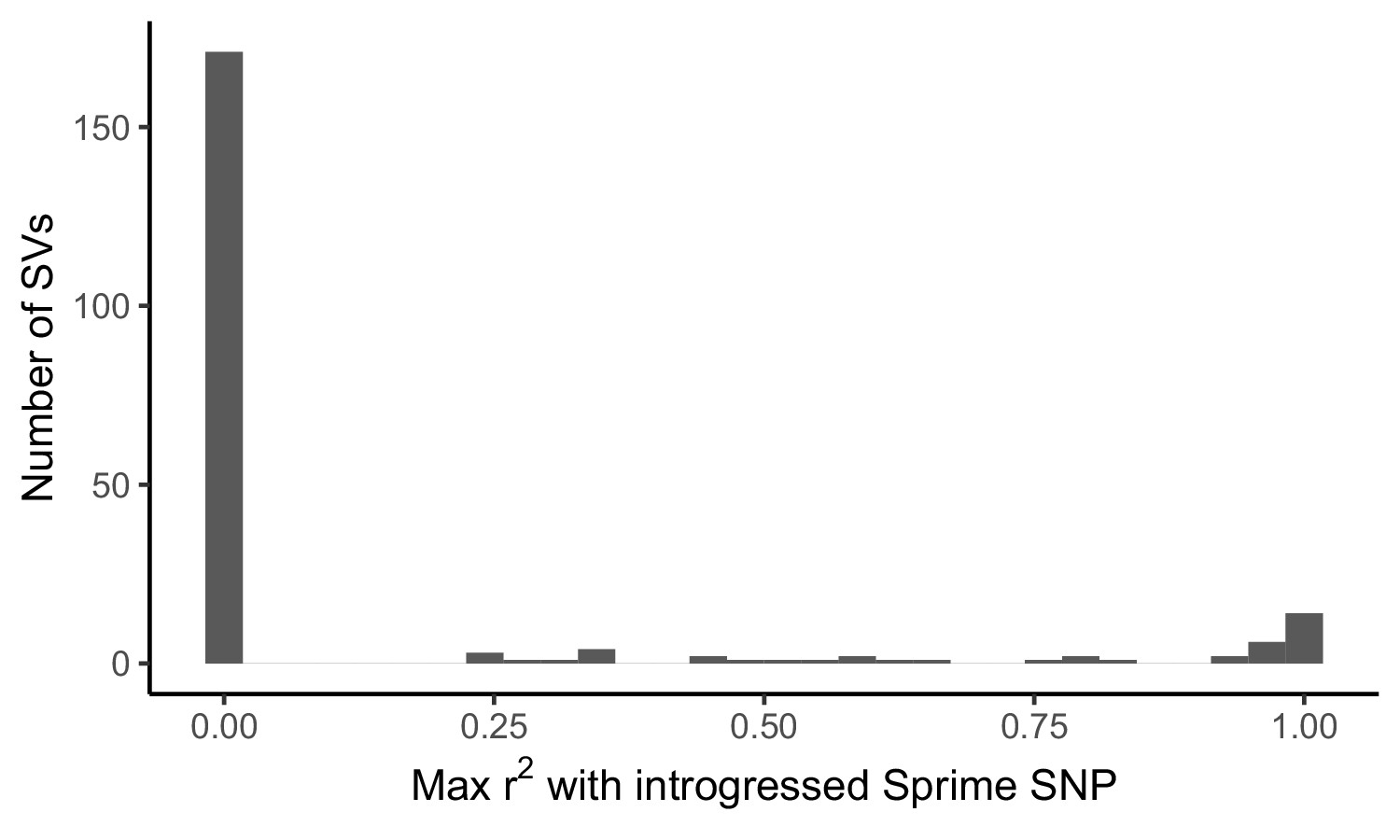
Distribution of LD between adaptive SVs and introgressed SNPs called by Sprime.
For the 215 most frequency differentiated SVs in our dataset, we calculated LD between the SV and SNPs defining introgressed haplotypes called by Sprime. LD calculations for each SV were restricted to one 1KGP population, chosen based on the ancestry component where the SV was found to exhibit branch-specific differentiation. We identified 26 candidate adaptively introgressed SVs, which had r2 > 0.5 with an introgressed SNP and were at low frequency (AF < 0.01) within African populations (excluding admixed ASW and ACB populations).
Figure 4—figure supplement 3
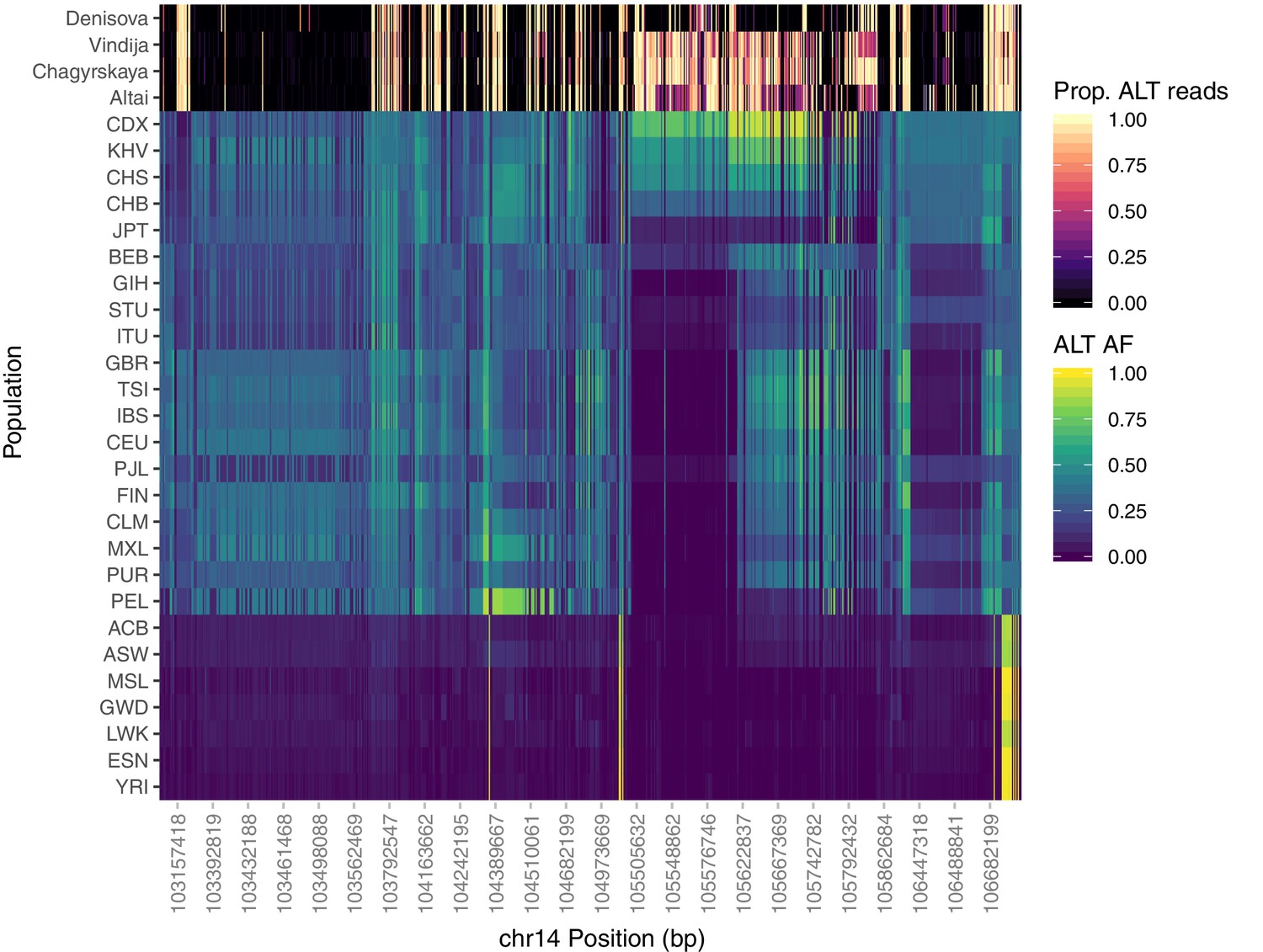
Population-specific allele frequencies in the broader IGH region.
The top four rows depict the proportion of aligned reads supporting the alternative allele at each SNP queried for the archaic aDNA samples. The remainder of rows depict the alternate allele frequency of each SNP within each of the 26 populations of 1KGP. Analysis was restricted to SNPs that are rare (MAF < 0.05) among African populations, but common within one or more Eurasian populations (MAF > 0.3).
Figure 4—figure supplement 4
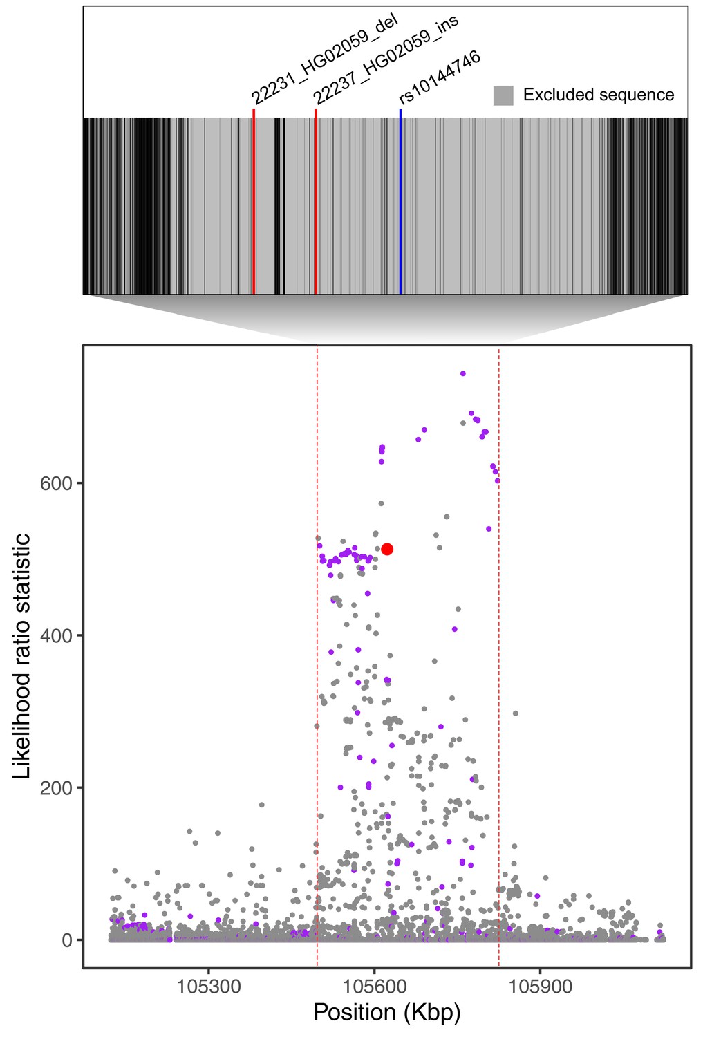
Filtering of Neanderthal-introgressed alleles at the IGH locus.
The bottom plot, identical to Figure 4A, shows likelihood ratio statistics (LRS) in the adaptive haplotype around the 33 bp IGHG4 insertion (red dot). The top inset shows the Altai Neanderthal mask (gray), used by Browning et al., 2018 to filter out sites with low-coverage or mapping quality. Positions of the two outlier SVs we identify in this region are represented by red lines. An introgressed SNP highlighted by Browning et al., 2018 is represented by the blue line.
Figure 4—figure supplement 5
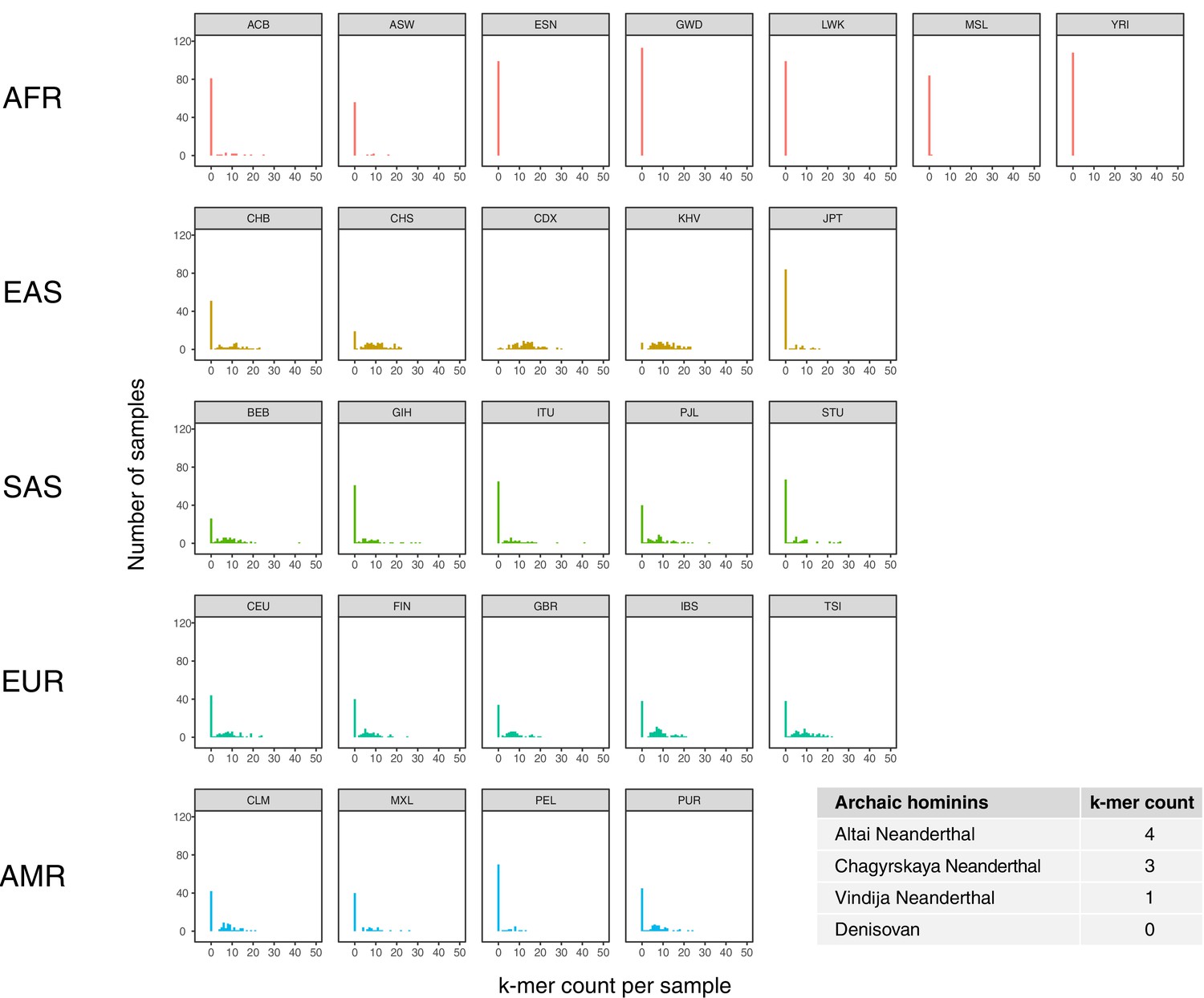
Population distribution of IGHG4 insertion using a diagnostic sequence.
Histograms show counts of a 48 bp sequence that is diagnostic of the 33 bp IGHG4 insertion per individual across the 1KGP dataset, stratified by population. Inset table depicts the counts of the diagnostic sequence in three high-coverage Neanderthal genomes and a high-coverage Denisovan genome.
Figure 4—figure supplement 6
Signatures of archaic introgression based on calls from Sprime.
For all variants with likelihood ratio statistic (LRS) > 450 at the IGH locus, we determined whether these variants fell on Sprime-inferred introgressed haplotypes in individuals of each of five 1KGP populations. Gray bars represent variants that were not identified by Sprime as introgressed, including short indels that were not included in the analysis by Browning et al., 2018. Cells are shaded black if the haplotype possesses the putative archaic allele at that variant, and white otherwise. The red bars represent two SVs with the highest LRS in the study.
Figure 4—figure supplement 7
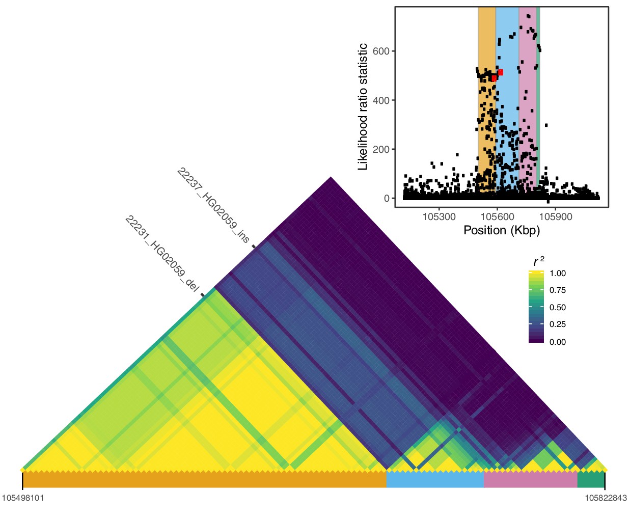
Local LD at the IGH locus.
We calculated pairwise LD between all variants with likelihood ratio statistic (LRS) >450 at the IGH locus, including the two SVs with the highest LRS in our study (22231_HG02059_del, 22237_HG02059_ins; red dots in the inset plot). Visualization of this LD matrix revealed at least four distinct blocks of LD, represented as colored rectangles below the LD heatmap and in the inset plot.
Figure 4—figure supplement 8
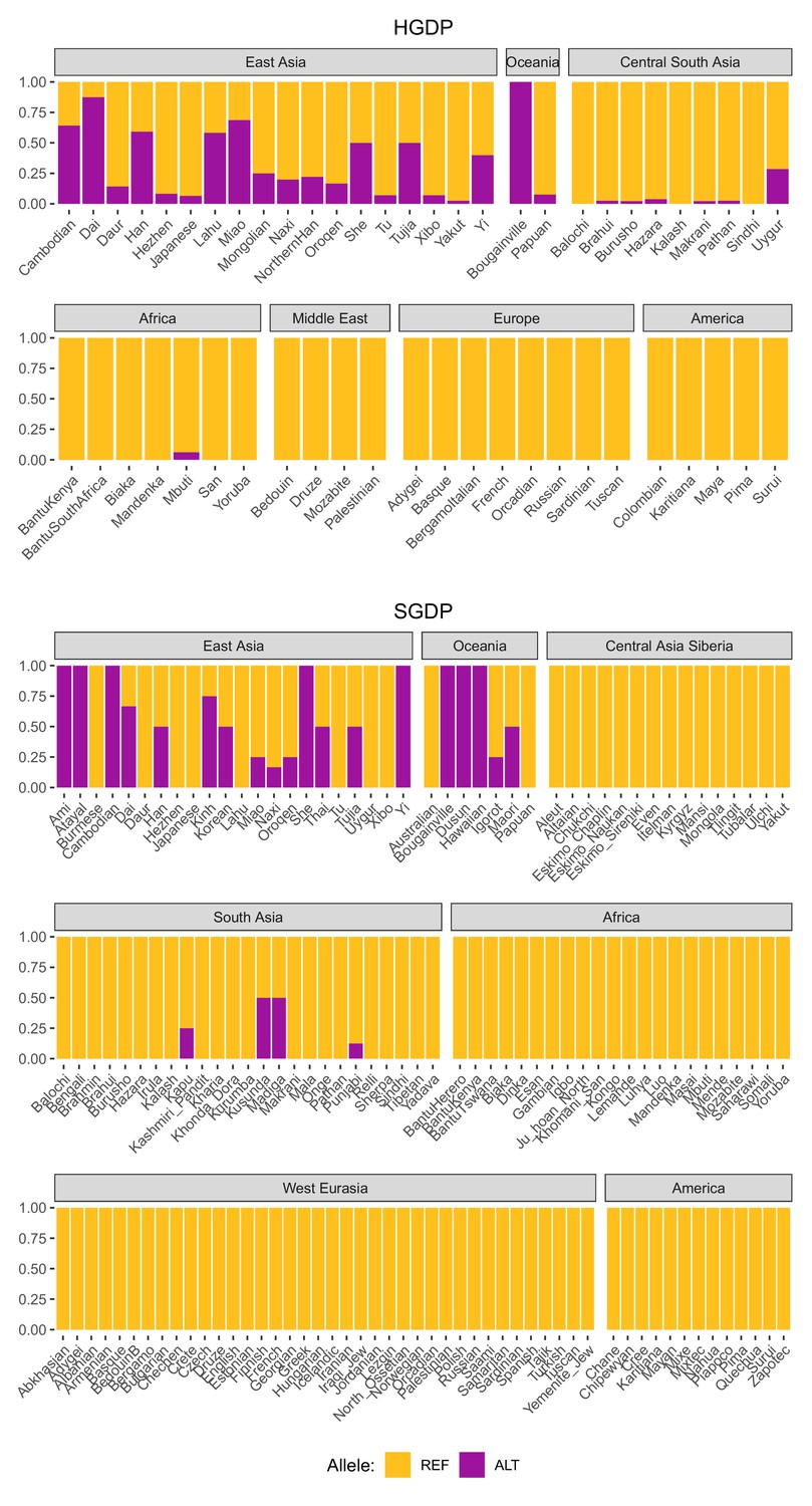
Global allele frequencies of the introgressed IGH haplotype.
Allele frequencies of rs150526114, a SNP that tags the IGH haplotype and IGHG4 insertion, based on data from the Human Genome Diversity Project (HGDP) and the Simons Genome Diversity Project (SGDP).
Figure 5 with 2 supplements
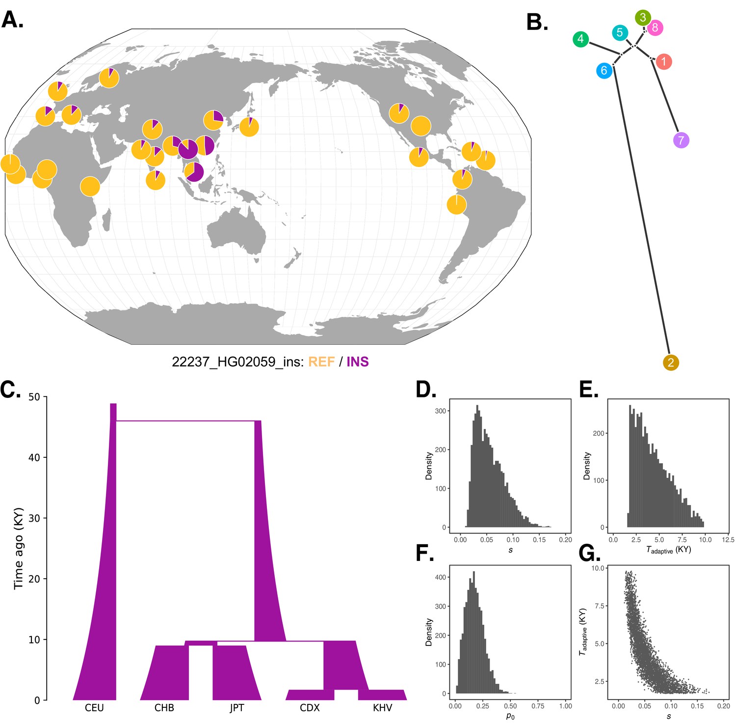
Local adaptation at the IGH locus.
(A) Population-specific frequencies of the putative Neanderthal-introgressed insertion allele in each of the 1KGP populations, in the style of the Geography of Genetic Variants browser (Marcus and Novembre, 2017). (B) Tree representation of the best-fit selection hypothesis for Neanderthal-introgressed haplotype tagged by the IGHG4 insertion polymorphism, as computed by Ohana. (C) Five-population demographic model used for simulation and parameter inference via approximate Bayesian computation (ABC). Population sizes and split times are further described in Materials and methods. (D) Posterior distribution of the selection coefficient (s). (E) Posterior distribution of the timing of the onset of selection (Tadaptive). (F) Posterior distribution of the initial allele frequency at the beginning of the simulation (p0). (G) Negative relationship between s and Tadaptive for simulations retained by ABC.
-
Figure 5—source data 1
Parameters and summary statistics for the simulations retained in the ABC analysis, underlying Figure 5D–G.
Simulation parameters are provided in the first three columns. Population-specific allele frequencies output by the simulation are provided in the last five columns, labeled by their corresponding 1KGP population codes.
- https://cdn.elifesciences.org/articles/67615/elife-67615-fig5-data1-v3.txt
Figure 5—figure supplement 1
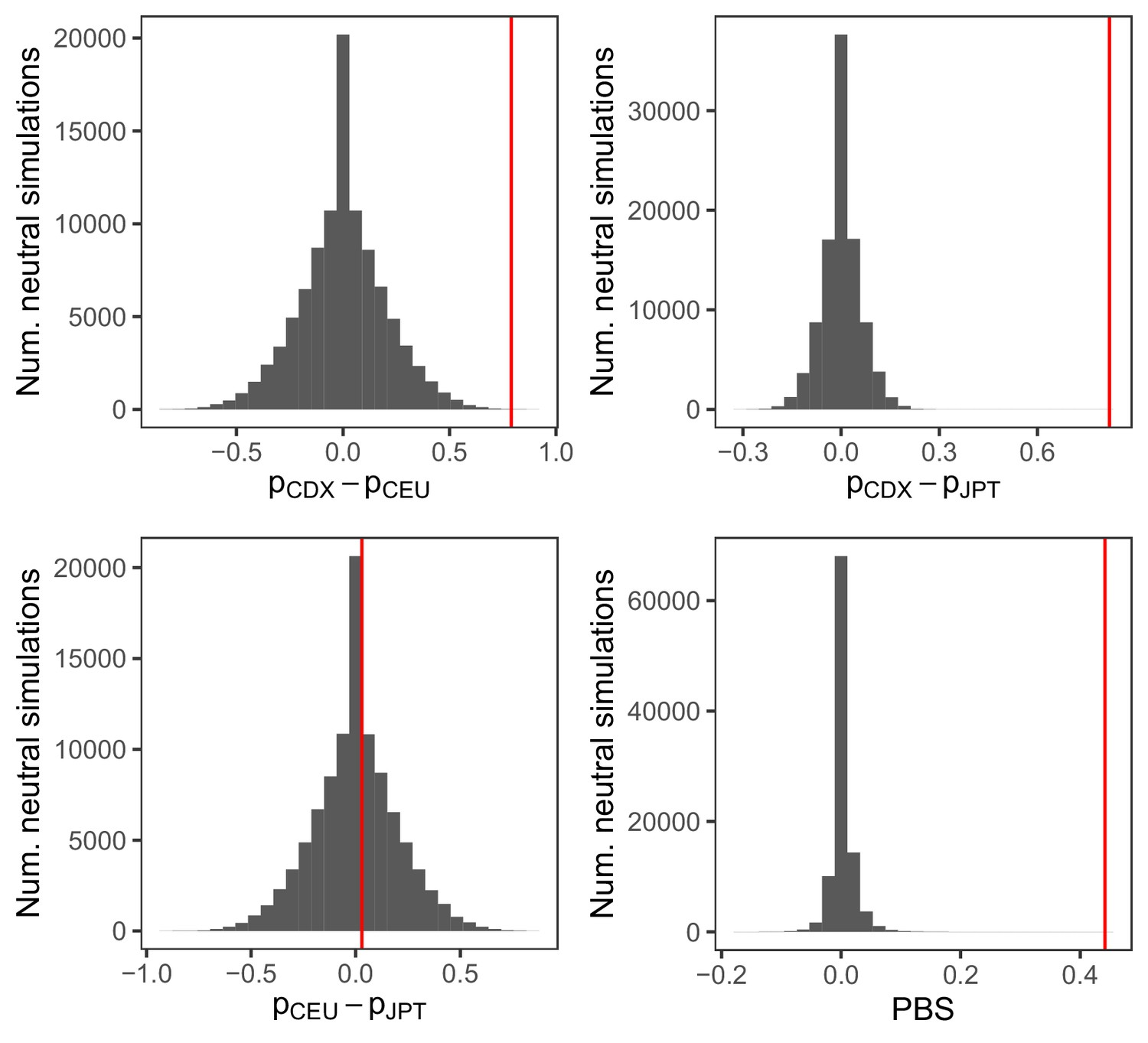
Distribution of FST and population branch statistic (PBS) for the IGHG4 insertion from 100,000 neutral simulations.
PBS was calculated between the Chinese Dai (CDX), Northern Europeans from Utah (CEU), and Japanese (JPT) populations, as . The red vertical lines represent the observed pairwise allele frequency differences and PBS for the insertion allele.
Figure 5—figure supplement 2
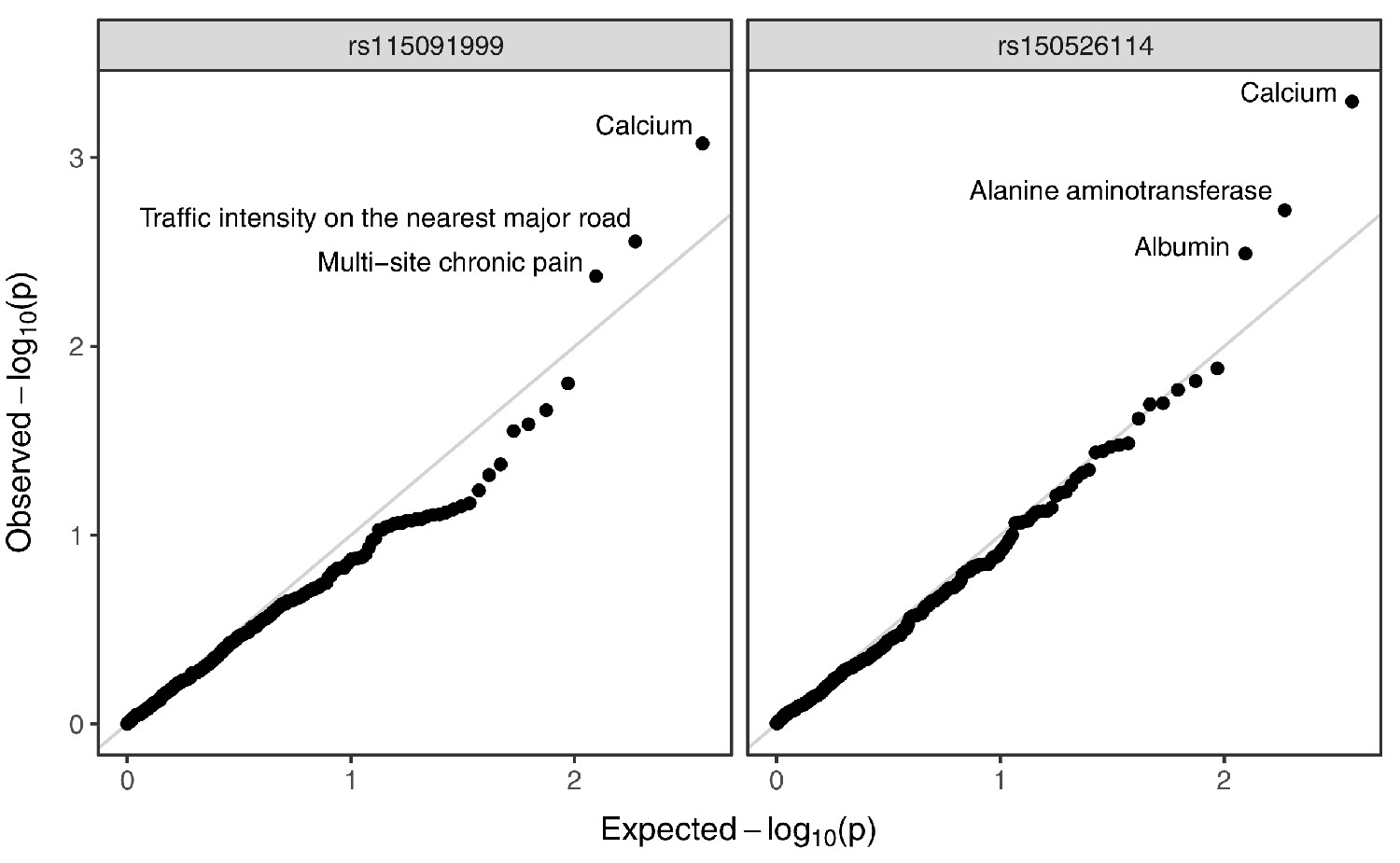
Annotated Q–Q plot from a phenome-wide association analysis of putative Neanderthal-introgressed variants at the IGH locus, using summary statistics from East Asian individuals from the pan-ancestry GWAS of the UK Biobank dataset.
SNP rs115091999 (left panel) tags 22231_HG02059_del, while rs150526114 (right panel) tags 22237_HG02059_ins within the CDX population. No phenotype association is significant after multiple testing correction (Bonferroni-adjusted p-value > 0.05).
Additional files
-
Supplementary file 1
Highly differentiated SV loci across ancestry components.
The top three SVs per ancestry component are reported. The IGH insertion and deletion are highlighted in bold text.
- https://cdn.elifesciences.org/articles/67615/elife-67615-supp1-v3.docx
-
Supplementary file 2
Highly differentiated SVs that are also significant eQTLs.
- https://cdn.elifesciences.org/articles/67615/elife-67615-supp2-v3.docx
-
Supplementary file 3
Highly differentiated SVs in LD (r2 >0.5) with putative archaic introgressed haplotypes called by Sprime.
The IGH insertion and deletion are highlighted in bold text.
- https://cdn.elifesciences.org/articles/67615/elife-67615-supp3-v3.docx
-
Transparent reporting form
- https://cdn.elifesciences.org/articles/67615/elife-67615-transrepform1-v3.docx
Download links
A two-part list of links to download the article, or parts of the article, in various formats.
Downloads (link to download the article as PDF)
Open citations (links to open the citations from this article in various online reference manager services)
Cite this article (links to download the citations from this article in formats compatible with various reference manager tools)
Local adaptation and archaic introgression shape global diversity at human structural variant loci
eLife 10:e67615.
https://doi.org/10.7554/eLife.67615


