In silico-labeled ghost cytometry
- Thinkcyte Inc, Japan
- Center for Advanced Intelligence Project, RIKEN, Japan
- The University of Tokyo, Japan
- BioResource Research Center, RIKEN, Japan
- Sysmex Corporation, Japan
- Juntendo University, Japan
- PRESTO, Japan Science and Technology Agency, Japan
Figures
Figure 1 with 3 supplements
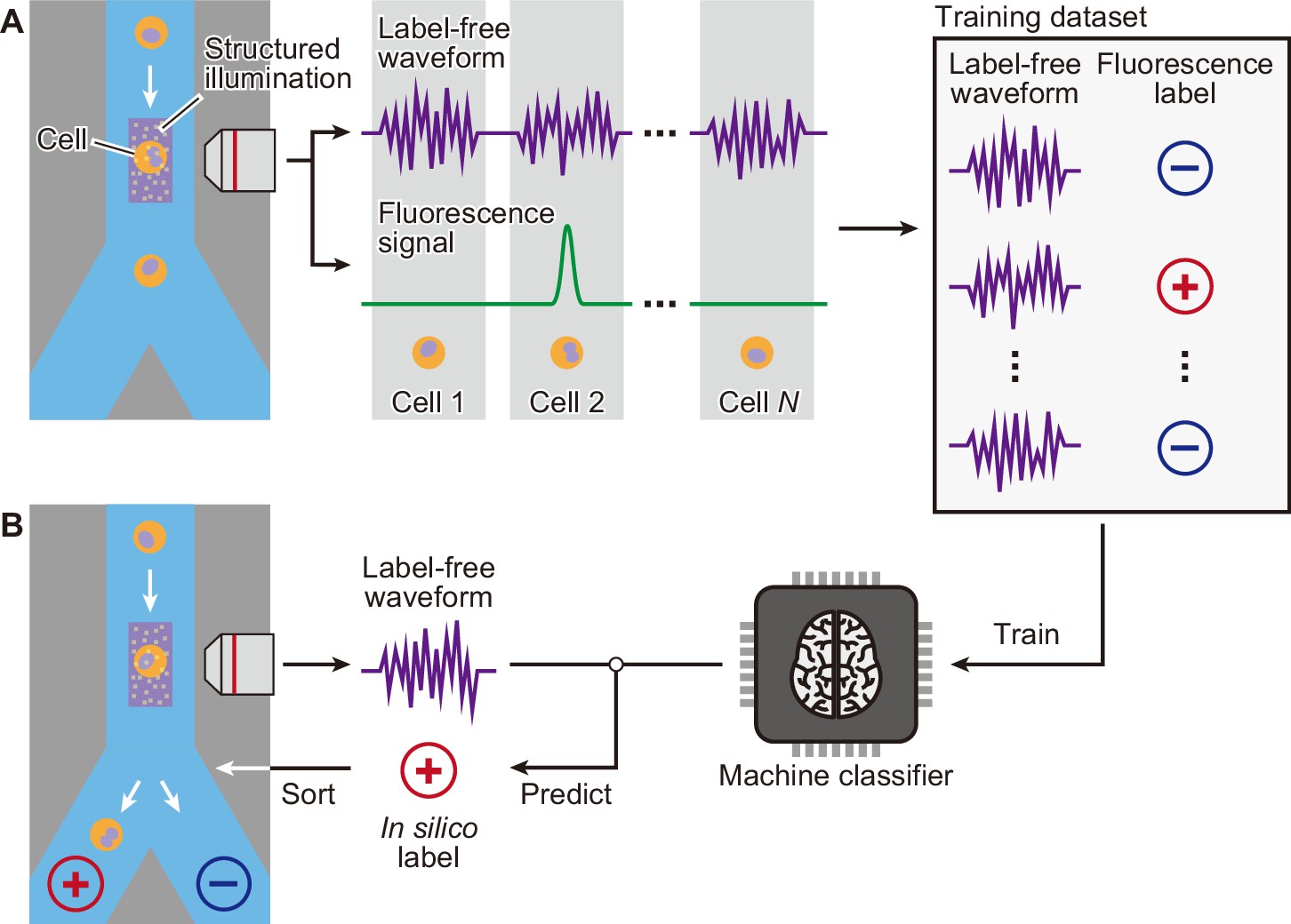
Schematic of iSGC to analyze and sort cells based on machine-predicted labels.
(A) First, the training data set is prepared by simultaneously acquiring the stain-free waveform and the fluorescence signal from each cell. Using the fluorescence intensity obtained from the fluorescence signal, each cell is labeled as positive or negative according to a defined threshold of the fluorescence intensity. The machine classifier is trained using this data set comprised of stain-free waveforms and fluorescence labels. (B) Once trained, in turn, the classifier can predict the fluorescence label in silico from the stain-free waveforms and sort the cells upon this prediction in real time. iSGC, in silico-labeled ghost cytometry.
Figure 1—figure supplement 1
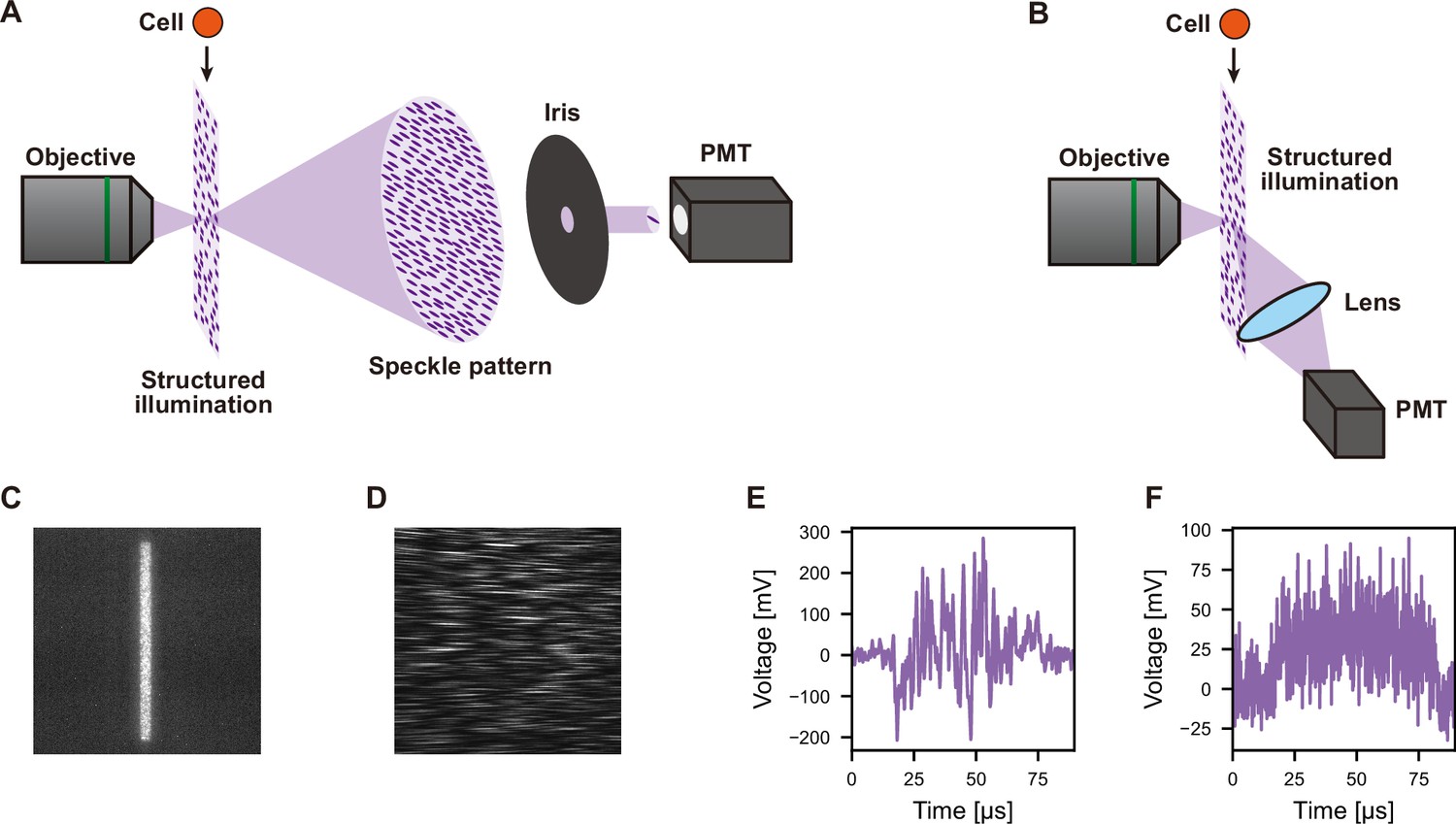
Principle of dGMI and ssGMI.
(A) Schematic of dGMI. A structured illumination is created using a coherent light at the focus of an objective. After the focus, the coherent light spreads out and creates a speckle pattern due to diffraction. At a substantial length away from the focus, the speckle pattern is large enough so that with an iris, a single to a few fringe patterns can be obtained while the rest is blocked. This small portion of the original speckle pattern is detected with a PMT. When a cell passes through the structured illumination, the phase and intensity changes in the transmitted light result in a change in the speckle pattern. This leads to a change in the intensity of the light detected at the PMT. Therefore, from the modulation of the detected signal, the phase and intensity information of the cell can be obtained. (B) Schematic of ssGMI. A structured illumination is created using a coherent light at the focus of an objective. Similar to the fluorescence in previously reported ghost cytometry (Ota et al., 2018), when the cell passes through the structured illumination, the side scatter resulting from the overlap of the cell with the structured illumination is directed orthogonal to the illumination light path. This is collected with a lens and detected by a PMT (see also Figure 1—figure supplement 3). In the case of bsGMI, the scattered light is collected behind the objective using a knife-edge mirror to separate from the illumination path (Figure 1—figure supplement 2). (C) Image of a structured illumination used for dGMI and ssGMI, obtained using a fluorescence film and a camera. (D) Image of a speckle pattern for dGMI, obtained using a camera. (E, F) Actual signal waveform of dGMI (E) and ssGMI (F). In both cases, the image of the cell cannot be obtained from the signal because the information from the cell is reduced for high throughput. bsGMI, back scatter ghost motion imaging; dGMI, diffractive ghost motion imaging, PMT, photomultiplier tube; ssGMI,side scatter ghost motion imaging.
Figure 1—figure supplement 2
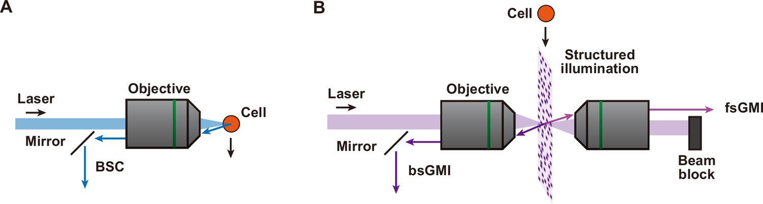
Principle of BSC, bsGMI, and fsGMI.
(A) Schematic of BSC. An illumination laser is focused onto a cell in flow. The BSC from a cell is obtained from the same side of the sample as the illumination. A mirror is used to separate the illumination laser and the BSC light. A BSC signal is similar to SSC, and BSC is used in place of SSC when it is difficult to position a collecting lens next to the channel and orthogonal to the illumination light, for instance, when using a microfluidic device. (B) Schematic of bsGMI and fsGMI. For bsGMI and fsGMI, a similar concept to BSC and FSC, respectively, is used except the illumination is a structured illumination. A bsGMI signal is similar to ssGMI, and bsGMI is used in place of ssGMI for the same reason as BSC. BSC, back scatter; bcGMI, XXX; FSC, forward scatter; fsGMi, XXX; SSC, side scatter.
Figure 1—figure supplement 3
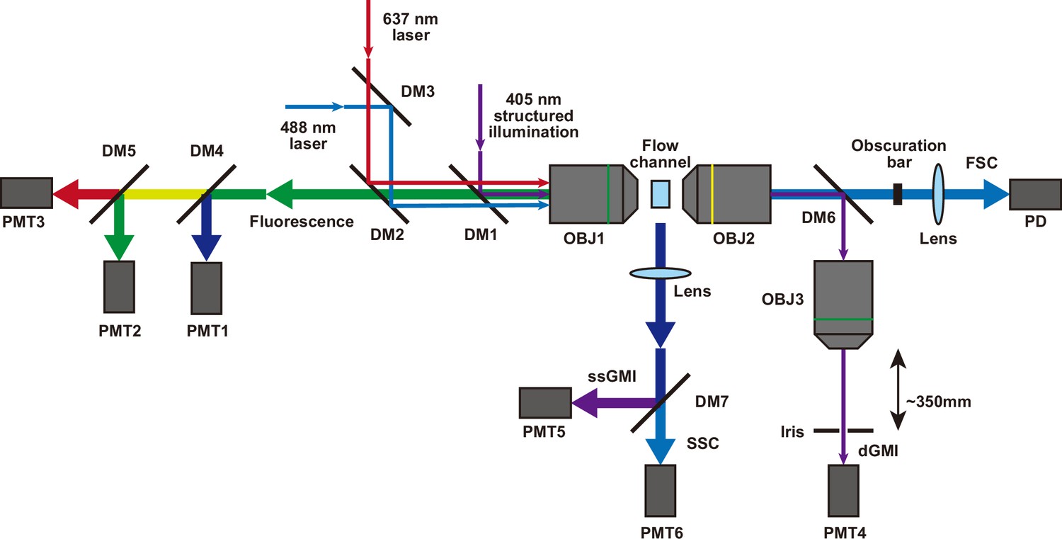
Optical system for iSGC.
dGMI was measured using a structured illumination created with a 405 nm laser source (Stradus 405-250, Vortran). The structured illumination was combined with other light sources using a dichroic mirror (DM1, ZT405rdc, Chroma) and focused on the flow channel using a 20× objective (OBJ1, UPLSAPO 20×, Olympus). The transmitted structured illumination was collected with a 10× objective (OBJ2, UPLFLN 10×, Olympus) and separated from other transmitted light using a dichroic mirror (DM6, ZT405rdc, Chroma). This was further passed through a 20× objective (OBJ3, UPLSAPO 20×), and in front of the objective at a distance of ~350 mm, an iris was put at an aperture size of ~3 mm. The light that entered the iris was detected with a PMT (PMT4) with a bandpass filter (405 nm, ET405/10×, Chroma) in front of it. ssGMI was measured using the same structured illumination as dGMI. However, instead of collecting the transmitted light, the scattered light from the flow channel orthogonal to the illumination light was collected using a plano-convex lens (f=50 mm, Thorlabs). Then it was separated from other scattered light using a dichroic mirror (DM7, ZT405rdc, Chroma) and detected with a PMT (PMT5) with a bandpass filter (ET405/10×, Chroma) in front of it. Fluorescence labels for training and validation were measured with either the 405 nm structured illumination, a 488 nm laser (Cobolt), or a 635 nm laser (Stradus 637-140, Vortran). The 488 nm laser and 637 nm laser were combined with a dichroic mirror (DM3, ZT488rdc), reflected with another dichroic mirror (DM2, ZT405/488/635rpc) for separating the returning fluorescence light, and combined with the 405 nm structured illumination with DM1. The three light sources were focused on the flow channel using OBJ1. The fluorescence was collected using the same objective and passed through DM1 and DM2. This was further separated into different colors with dichroic mirrors DM4 and DM5 and detected using PMTs (PMT1, PMT2, and PMT3) with different bandpass filters (ET440/40×, ET525/50m, ET675/50m, respectively, all from Chroma) in front of them. In the case of WBC differential classification, a similar setup for four-color detection using three dichroic mirrors and four PMTs was used. Forward scatter (FSC) and side scatter (SSC) for triggering acquisition and initial cell population gating were measured using the 488 nm laser or the 637 nm laser. The figure is depicted for the case of the 488 nm laser. For the FSC, from the flow channel, the transmitted 488 nm light was collected with OBJ2 and passed through DM6. Then the main transmitted beam was blocked with an obscuration bar, and the scattered light that came around the obscuration bar was collected with a lens and detected with a photodetector (PDA100A, Thorlabs) with a bandpass filter (ZET488/10×, Chroma) in front of it. For the SSC, the scattered light from the flow orthogonal to the illumination light was collected using a plano-convex lens (f=50 mm, Thorlabs). Then it was passed through DM7 and collected with a PMT (PMT6) with a bandpass filter (ZET488/10×, Chroma) in front of it. dGMI, diffractive ghost motion imaging; iSGC, in silico-labeled ghost cytometry; PMT, photomultiplier tube; ssGMI, XXX.
Figure 2 with 2 supplements

Label prediction and cell sorting with iSGC using cell line samples.
(A) Histogram of FSC for HeLa S3 (blue) and MIA PaCa-2 (red) cells. The intensity of FSC reflects the size of cells. There is a large overlap of the two cell-line populations, showing that the two cell lines are similar in size. (B) Fluorescence intensity evaluation of HeLa S3 and MIA PaCa-2 cells before sorting. The population with lower green fluorescence intensity corresponds to HeLa S3 cells while the population with higher fluorescence intensity corresponds to MIA PaCa-2 cells. (C) SVM score histogram for the classification of HeLa S3 and MIA PaCa-2 cells obtained by iSGC as in silico-predicted labels during sorting. Blue and red colors assigned in the histogram correspond to the cells labeled as HeLa S3 and MIA PaCa-2 cells, respectively, derived from the green fluorescence obtained simultaneously for validation. The dashed line shows the decision boundary by the SVM. (D) A receiver operating characteristic curve for the classification of HeLa S3 and MIA PaCa-2 cells using dGMI during sorting. The AUC for the classification with dGMI was 0.963, showing a high classification ability. (E) Fluorescence intensity evaluation of HeLa S3 and MIA PaCa-2 cells after sorting. The concentration of MIA PaCa-2 cells was enriched from 60.3% (B) to 97.3% (E). dGMI, diffractive ghost motion imaging; FSC, forward scatter; iSGC, in silico-labeled ghost cytometry; SVM, support vector machine.
Figure 2—figure supplement 1
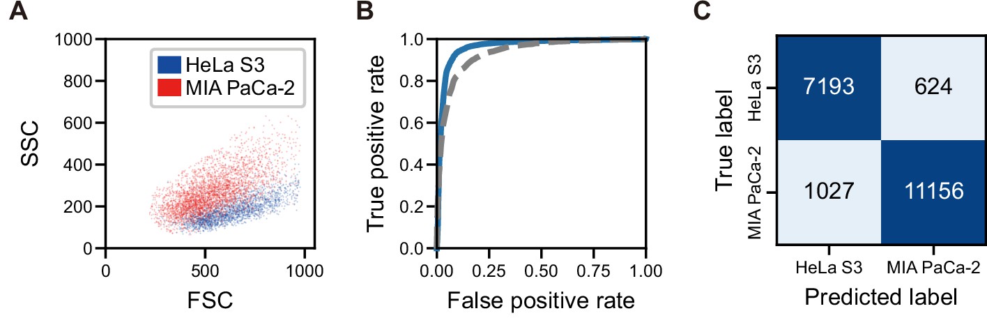
Comparison with FSC and SSC and confusion matrix for the sorting of HeLa S3 and MIAPaCa-2 cells with iSGC.
(A) Scatter plot of FSC and SSC for HeLa S3 (blue) and MIA PaCa-2 (red) cells. (B) ROC curve for the SVM-based classification of HeLa S3 and MIA PaCa-2 cells using dGMI during sorting (blue solid line) and FSC and SSC intensities (gray dashed line). The AUC for the classification with dGMI was 0.963, showing a high classification ability, whereas the AUC for the classification with FSC and SSC intensities was 0.936±0.005, showing limited performance. (C) Confusion matrix for the classification of HeLa S3 and MIA PaCa-2 cells during sorting. The classification accuracy is 0.917, and the purity of MIA PaCa-2 cells derived from only the classification is 94.7%. We assume that the purity of the sorted cells (97.3%) slightly deviates from this due to sorting errors and statistical errors. dGMI, diffractive ghost motion imaging; FSC, forward scatter; iSGC, in silico-labeled ghost cytometry; ROC, receiver operating characteristic; SSC, side scatter; SVM, support vector machine.
Figure 2—figure supplement 2
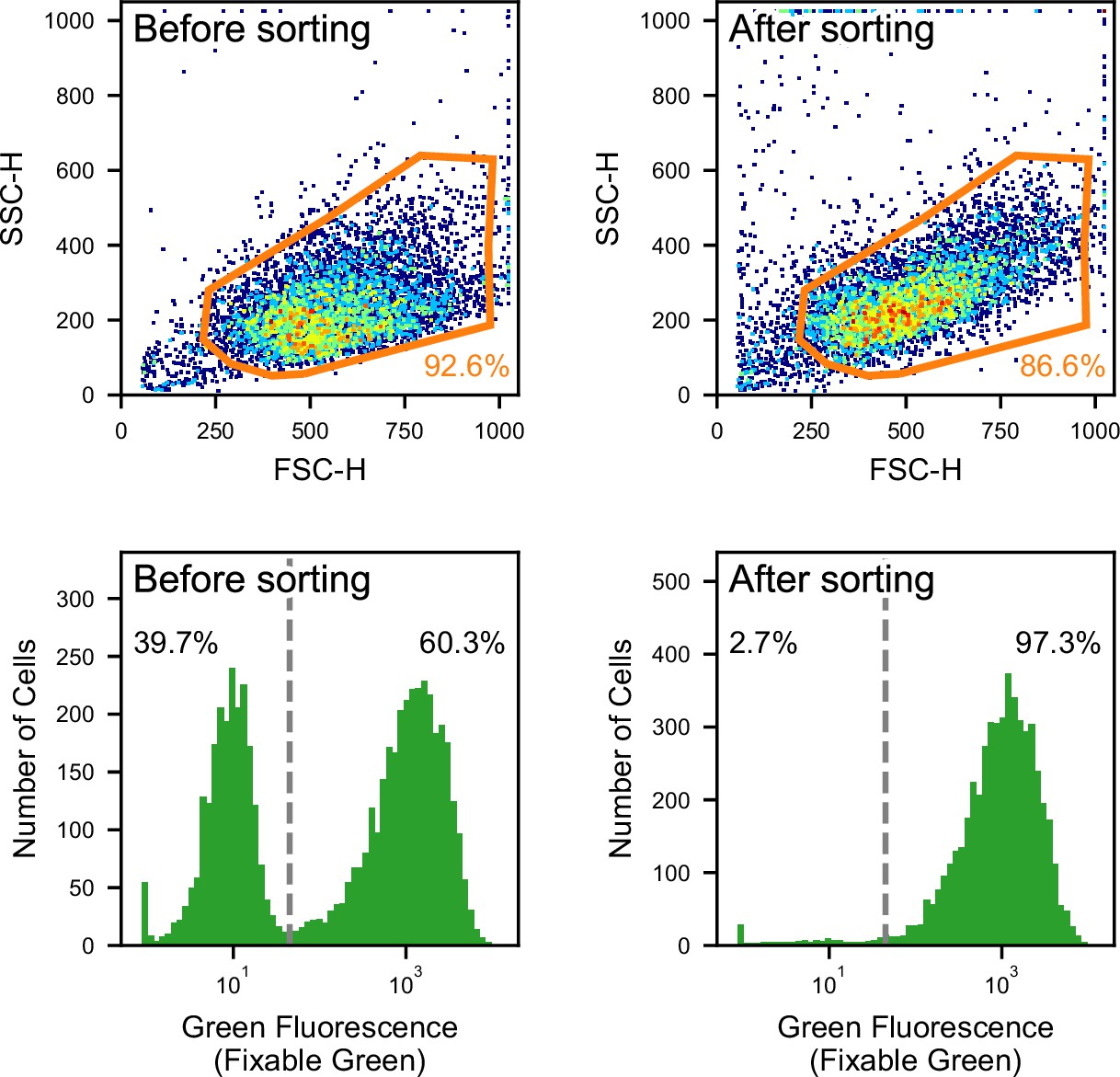
Gating for the flow cytometry analysis in the classification and sorting of HeLa S3 cells and MIA PaCa-2 cells.
FSC/SSC scatter plots used for removing debris and doublets (top panels) and fluorescence histogram for Fixable Green used for labeling positive (right) and negative (left) cells (bottom panels) before sorting and after sorting.
Figure 3 with 2 supplements

Classification of live, dead, and apoptotic iPSCs with iSGC.
(A). Scatter plot of PI and Annexin V for iPSCs. The population within the blue, red, and orange regions were labeled as live, dead, and apoptotic cells, respectively. (B). Scatter plot of FSC and BSC for iPSCs without exclusion of debris and doublets. (C). Scatter plot of FSC and BSC for each labeled iPSC populations. The blue, red, and orange dots each correspond to live, dead, and apoptotic cells, respectively. All populations, which are previously shown in (B), are gated prior to labeling for removing debris and doublets (Figure 3—figure supplement 1A and Figure 3—figure supplement 2). In the plot, the live and dead populations have distinct separation, but the live and apoptotic populations overlap. (D–F) SVM score histograms for the iSGC-based classification of dead cells from live cells (D), apoptotic cells from live cells (E), and apoptotic cells from live cells within the red region in the scatter plot (B, F). The colors correspond to the labels in (A). All histograms are the best result of 10 times random sampling. The AUCs for each classification were 0.999 (D), 0.885 (E), and 0.904 (F). The mean and standard deviation of AUCs for the 10 trials in each condition were 0.998±0.002, 0.877±0.007, and 0.891±0.012, respectively (Figure 3—figure supplement 1, D, E, and F). BSC, back scatter; FSC, forward scatter; iPSC, induced pluripotent stem cell; iSGC, in silico-labeled ghost cytometry; PI, propidium iodide; SVM, support vector machine.
Figure 3—figure supplement 1

Scatter plot, confusion matrices, and SVM score histograms for the classification of live, dead, and apoptotic cells using iPSCs with iSGC.
(A) Scatter plot of FSC and BSC intensities. Orange dashed line corresponds to the region used to label the cells in Figure 3A. Red solid line is the same region as the red line in Figure 3B. (B, C) Confusion matrices for the SVM-based classification of live, dead and apoptotic cells using dGMI and ssGMI (B) and FSC and SSC (C), derived by the sum of all trials from 10 times random sampling. The macro-average F1-scores were 0.842±0.006 (B) and 0.759±0.006 (C). (D–F). ROC curves for the classification of live versus dead cells (D), live versus apoptotic cells (E), and live versus apoptotic cells within the region of red line in (A). (F) Blue solid lines correspond to the SVM-based classification with dGMI and bsGMI, and gray dashed lines correspond to the SVM-based classification with FSC and BSC. Each line represents the mean, and the shaded area around each line represents the standard deviation for 10 trials. The AUCs of the blue solid line and the gray dashed line are 0.997±0.002 and 0.974±0.007, respectively, in (D), 0.878±0.007 and 0.779±0.011, respectively, in (E), and 0.892±0.012 and 0.777±0.012, respectively, in (F). BSC, back scatter; bsGMI, XXX; dGMI, diffractive ghost motion imaging; FSC, forward scatter; iPSC, induced pluripotent stem cell; iSGC, in silico-labeled ghost cytometry; ROC, receiver operating characteristic; ssGMI, XXX; SVM, support vector machine.
Figure 3—figure supplement 2
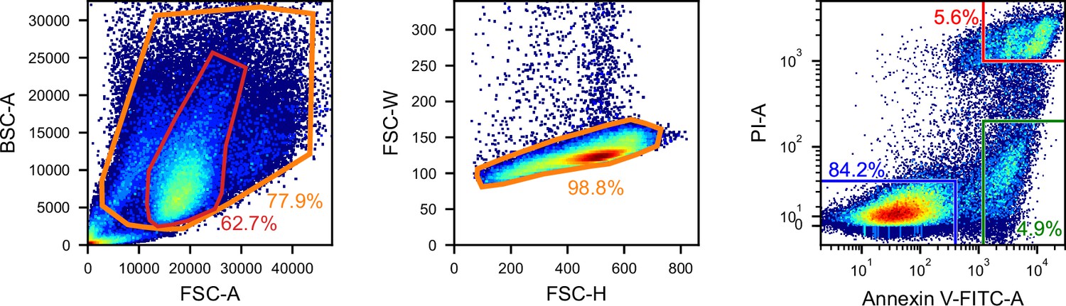
Gating for the iSGC analysis in the classification of live, dead, and apoptotic iPSCs.
FSC/BSC (left panel) and FSC height/width (middle panel) scatter plots used for removing debris and doublets, and fluorescence scatter plot of Annexin V-FITC and PI (right panel) for labeling live (blue), dead (red), and apoptotic (green) cells. The region in the red line is the same region as the red line in Figure 3B and Figure 3—figure supplement 1. BSC, back scatter; FSC, forward scatter; iSGC, in silico-labeled ghost cytometry; iPSC, induced pluripotent stem cell; PI, propidium iodide.
Figure 4 with 4 supplements
Actual fluorescence labels and predicted labels by iSGC for the classification of undifferentiated and cancer cells from iPSC-derived cells.
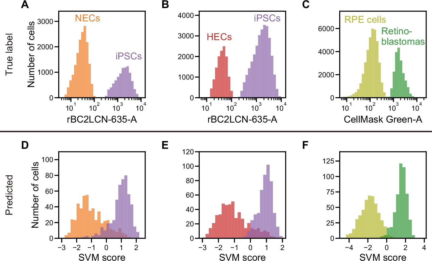
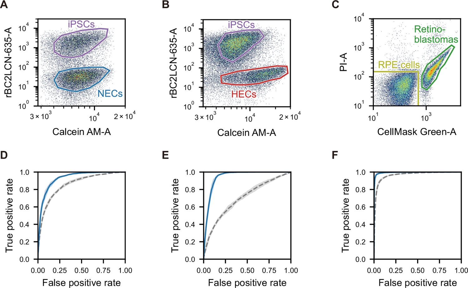
(A–C). Histograms of rBC2LCN-635 fluorescence intensity for a mixture of NECs (orange) and iPSCs (violet) (A), a mixture of HECs (red) and iPSCs (violet) (B), and a histogram of CellMask Green intensity for a mixture of RPE cells (light green) and retinoblastoma (green) (C). These markers were used for discriminating cells in a training data set. (D–F). SVM score histogram for the iSGC-based classification of NECs and iPSCs (D), HECs and iPSCs (E), and RPE cells and retinoblastoma (F) with dGMI and ssGMI. The colors correspond to the labels in (A), (B), and (C) used for validation. All histograms are the best result of 10 times random sampling. The AUCs for each classification were 0.943 (D), 0.951 (E), and 0.998 (F). The mean and standard deviation of AUCs for the 10 trials in each condition were 0.929±0.008, 0.942±0.007, and 0.994±0.002, respectively (Figure 4—figure supplement 1, D, E, and F). dGMI, diffractive ghost motion imaging; HEC, hepatic endodermal cell; iPSC, induced pluripotent stem cell; iSGC, in silico-labeled ghost cytometry; NEC, neuroectodermal cell; RPE, retinal pigment epithelium; ssGMI, side scatter ghost motion imaging; SVM, support vector machine.
Figure 4—figure supplement 1
Scatter plot gating and ROC curves for the classification of undifferentiated or cancer cells and iPSC-derived cells.
(A–C) Scatter plots of fluorescence intensity of Calcein AM and rBC2LCN-635 for the mixture of iPSCs and NECs (A) and iPSCs and HECs (B), and scatter plot of fluorescence intensity of CellMask Green and PI for mixture of RPE cells and retinoblastomas (C). The region in each plot is the actual gating used to label each type of cells and to exclude dead cells. (D–F) ROC curve for the classification of iPSCs and NECs (D), iPSCs and HECs (E), and RPE cells and retinoblastomas (F). Blue solid lines indicate the SVM-based classification using dGMI and ssGMI, and gray dashed lines indicate the SVM-based classification using FSC and SSC intensities. All ROC curves are means of 10 times random sampling. Each line represents the mean, and the shaded area around each line represents the standard deviation for 10 trials. The AUCs of the blue solid line and the gray dashed line are 0.929±0.008 and 0.857±0.009, respectively, in (D), 0.943±0.007 and 0.698±0.016, respectively, in (E), and 0.994±0.002 and 0.966±0.004, respectively, in (F). dGMI, diffractive ghost motion imaging; HEC, hepatic endodermal cell; iPSC, induced pluripotent stem cell; iSGC, in silico-labeled ghost cytometry; NEC, neuroectodermal cell; PI, propidium iodide; ROC, receiver operating characteristic; RPE, retinal pigment epithelium; ssGMI, XXX; SVM, support vector machine.
Figure 4—figure supplement 2
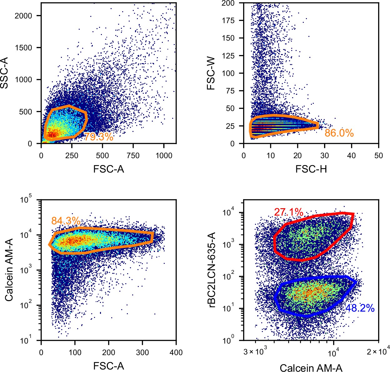
Gating for the iSGC analysis in the classification of iPSCs and NECs.
FSC/SSC (top-left panel) and FSC height/width (top-right panel) scatter plots used for removing debris and doublets, FSC and Calcein AM fluorescence scatter plot (bottom-left panel) for removing dead cells, and fluorescence scatter plot of Calcein AM and rBC2LCN-635 (bottom-right panel) for labeling undifferentiated (red) and differentiated (blue) cells. FSC, forward scatter; iPSC, induced pluripotent stem cell; iSGC, in silico-labeled ghost cytometry; NEC, neuroectodermal cell; SSC, side scatter.
Figure 4—figure supplement 3
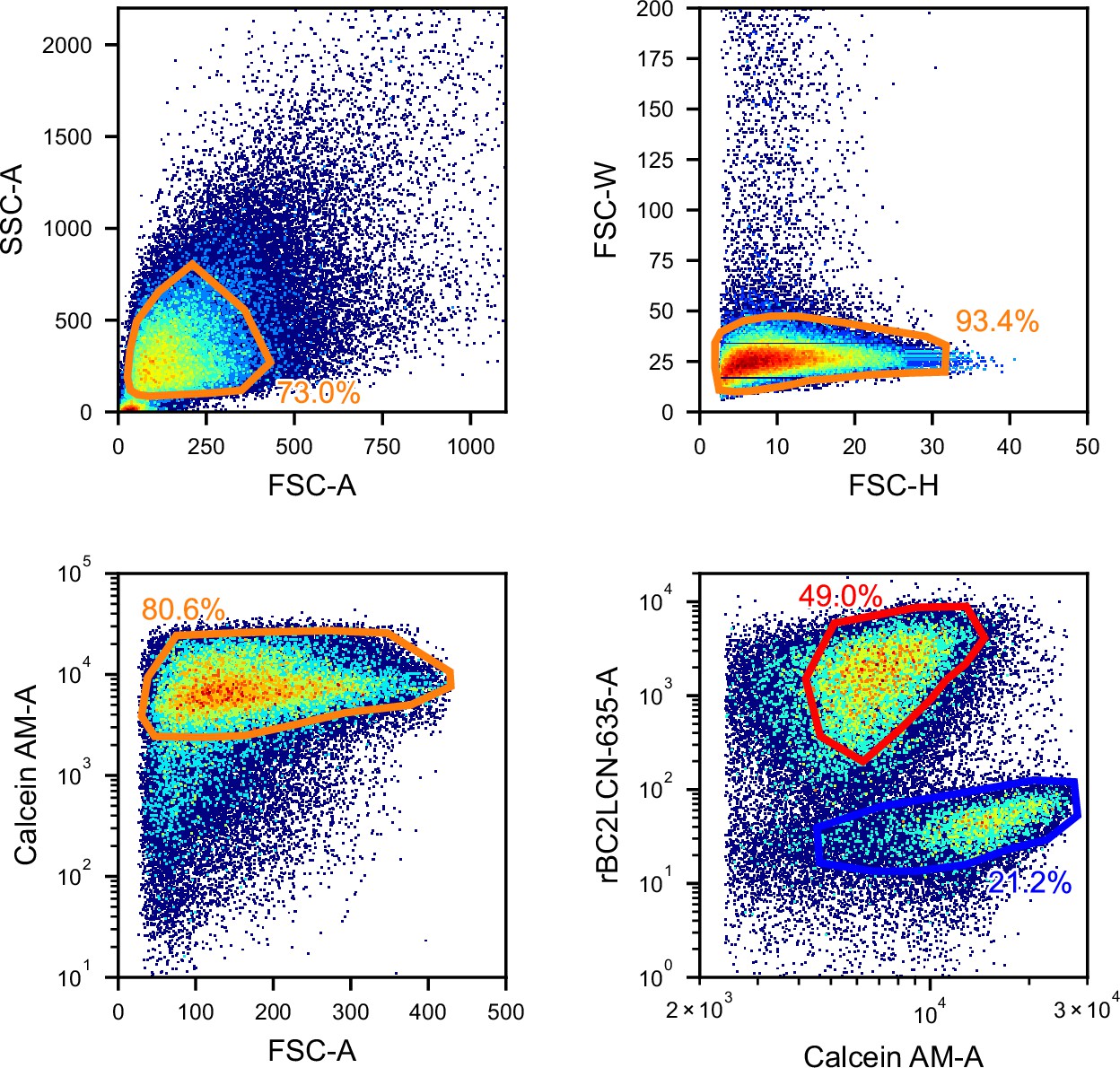
Gating for the iSGC analysis in the classification of iPSCs and HECs.
FSC/SSC (top-left panel) and FSC height/width (top-right panel) scatter plots used for removing debris and doublets, FSC and Calcein AM fluorescence scatter plot (bottom-left panel) for removing dead cells, and fluorescence scatter plot of Calcein AM and rBC2LCN-635 (bottom-right panel) for labeling undifferentiated (red) and differentiated (blue) cells. FSC, forward scatter; HEC, hepatic endodermal cell; iPSC, induced pluripotent stem cell; iSGC, in silico-labeled ghost cytometry; SSC, side scatter.
Figure 4—figure supplement 4
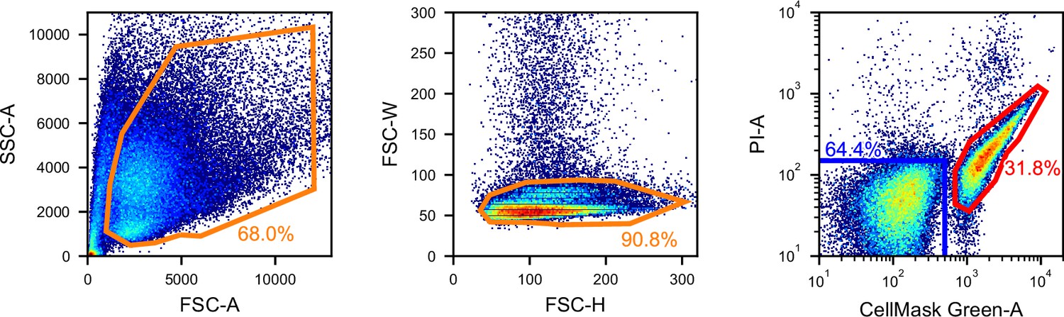
Gating for the iSGC analysis in the classification of RPE cells and retinoblastomas.
FSC/SSC (left panel) and FSC height/width (middle panel) scatter plots used for removing debris and doublets and fluorescence scatter plot of CellMask Green and PI (right panel) for simultaneously removing dead cells and labeling RPE cells (blue) and retinoblastomas (red). FSC, forward scatter; iSGC, in silico-labeled ghost cytometry; PI, propidium iodide; RPE, retinal pigment epithelium; SSC, side scatter.
Figure 5 with 3 supplements
Peripheral WBC differential classification with iSGC.
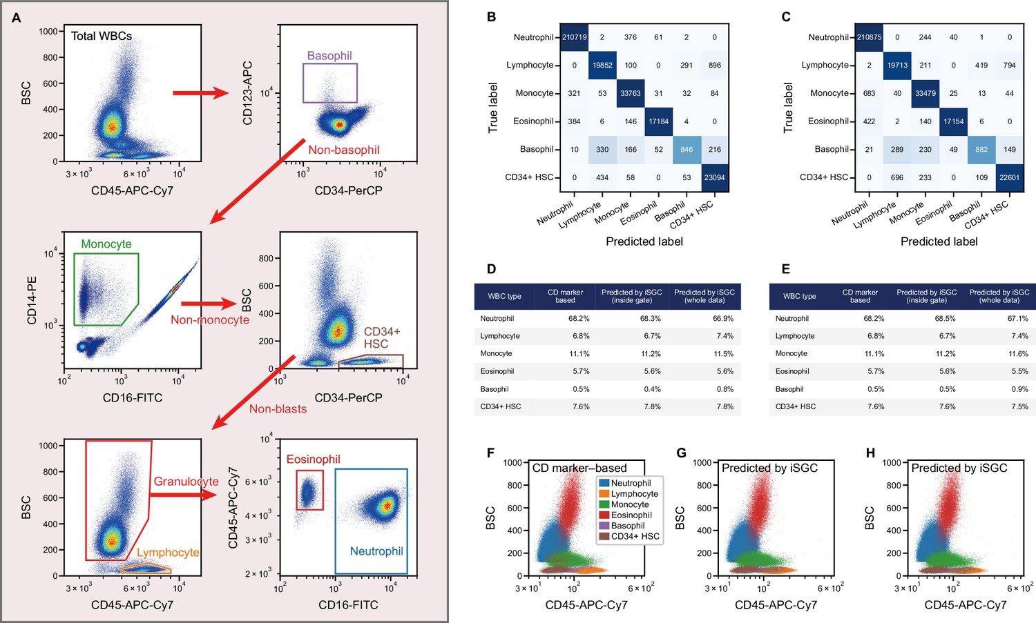
(A) Flow-cytometry scatter plots used for gating and labeling WBCs. (B, C) Confusion matrix for the classification of peripheral WBCs. The training and classification were performed using a sample from the same donor (intra-donor) for (B) and samples from different donors (inter-donor) for (C). The macro-average F1-scores were 0.911 and 0.904 for (B) and (C), respectively. (D, E) Proportion of each cell type by CD-marker-based labels, iSGC-predicted labels for cells that were gated and given the ground truth labels in (A), and iSGC-predicted labels for all cells including those that were not gated in (A). Similar to (B) and (C), the training and classification were performed in an intra-donor manner for (D) and an inter-donor manner for (E). (F–H). Scatter plot of CD45 and BSC for all WBC. The colors in each plot correspond to CD-marker-based labels (F), iSGC-predicted labels trained, and predicted in an intra-donor manner (G), and iSGC-predicted labels trained and predicted in an inter-donor manner (H). The colors in (G) and (H) correspond to the same labels as (F). BSC, back scatter; iSGC, in silico-labeled ghost cytometry; WBC, white blood cell.
Figure 5—figure supplement 1
Confusion matrix and proportion of cell types for WBC differential classification performed for a different donor sample.
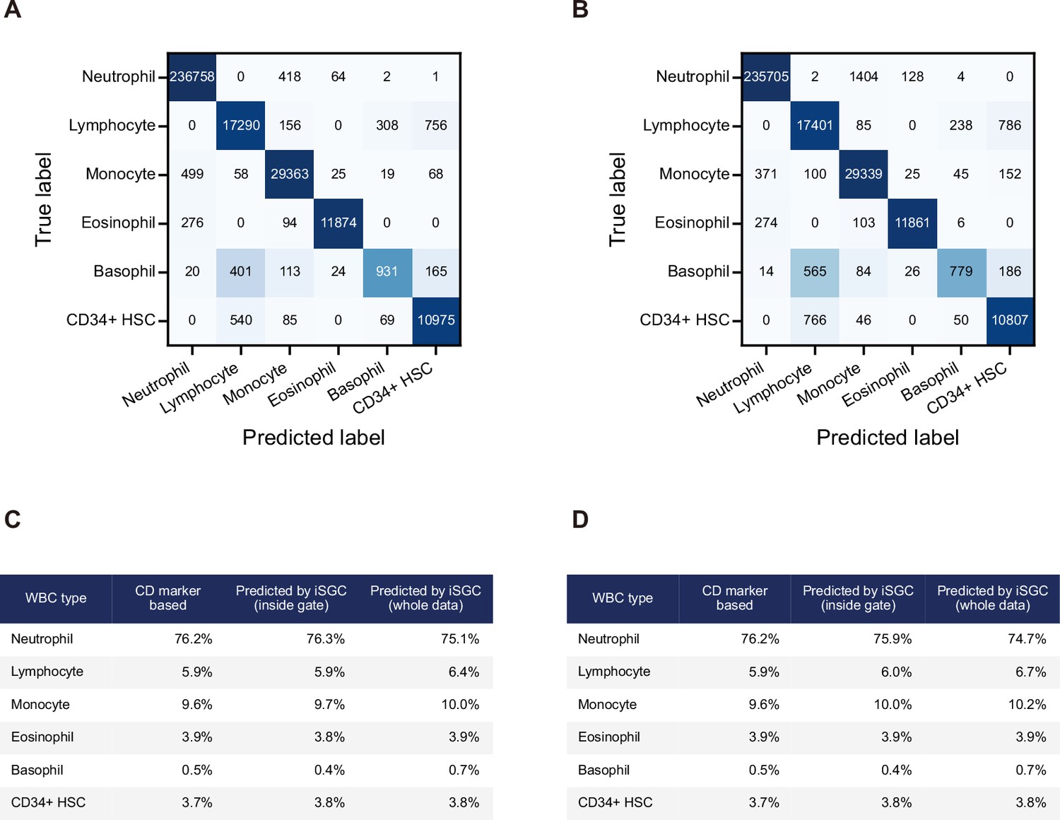
(A, B) Confusion matrix for the classification of peripheral WBCs performed on the donor blood sample used for training in Figure 5C and E. The training and classification were performed in an intra-donor manner for (A) and in an inter-donor manner for (B). The macro-average F1-scores were 0.907 and 0.890 for (A) and (B), respectively. These values are in close correspondence with those in Figure 5B and C. (C, D) Proportion of each cell type by CD-marker-based labels and iSGC-predicted labels for cells that were gated and given the ground truth labels, and iSGC-predicted labels for all cells including those that were not gated. Similar to (A) and (B), the training and classification were performed in an intra-donor manner for (C) and an inter-donor manner for (D). iSGC, in silico-labeled ghost cytometry; WBC, white blood cell.
Figure 5—figure supplement 2
Gating for a single run of blood cells obtained from a single donor used for providing the ground truth and performing intra-donor learning for the iSGC analysis in WBC differential classification.
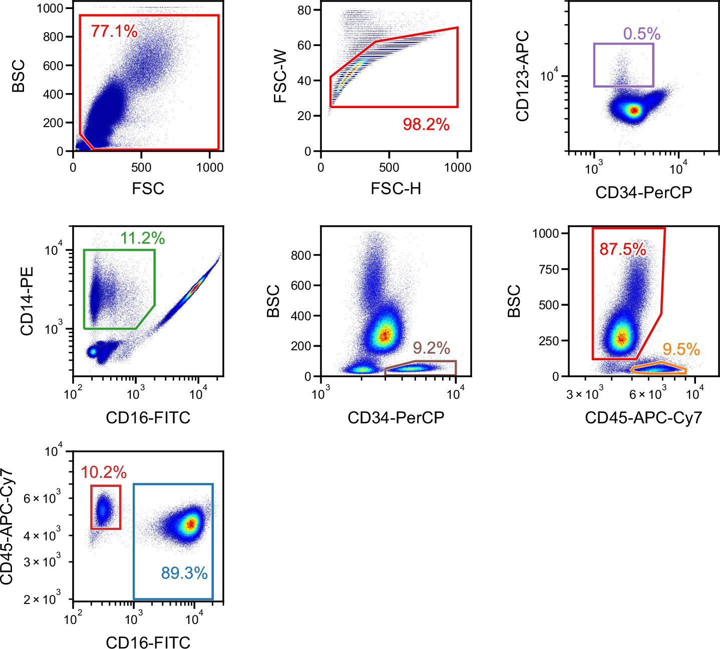
FSC/BSC (top-left panel) and FSC width/height (top-middle panel) scatter plots were used for removing debris and doublets. The rest of the panels correspond to the scatter plots in Figure 5A. First, CD34-PerCP/CD123-APC (top-right panel) was used to gate basophils. The non-basophils were then plotted on a CD16-FITC/CD14-PE scatter plot (second row, left panel) to gate monocytes. The non-monocytes were then plotted on a CD34-PerCP/BSC scatter plot (second row, middle panel) to gate the CD34+ hematopoietic stem cells (HSCs). The non-HSCs were then plotted on a CD45-APC-Cy7-H/BSC scatter plot (second row, right panel) to gate lymphocytes (lower right gate) and granulocytes (upper-left gate). The granulocytes were then plotted on a CD16-FITC/CD45-APC-Cy7-A plot (bottom-left panel) to gate eosinophils (upper-left gate) and neutrophils (lower-right gate). BSC, back scatter; FSC, forward scatter; iSGC, in silico-labeled ghost cytometry; WBC, white blood cell.
Figure 5—figure supplement 3
Gating for a single run of blood cells obtained from a different donor used for performing inter-donor learning for the iSGC analysis in WBC differential classification.
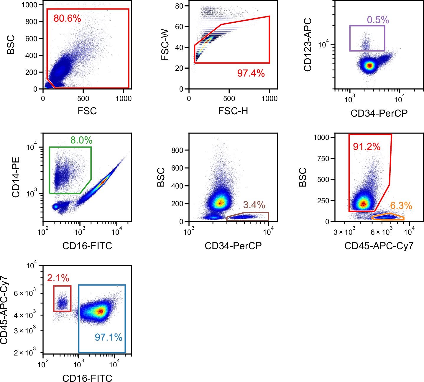
FSC/BSC (top-left panel) and FSC width/height (top-middle panel) scatter plots were used for removing debris and doublets. The rest of the panels correspond to the scatter plots in Figure 5A. First, CD34-PerCP/CD123-APC (top-right panel) was used to gate basophils. The non-basophils were then plotted on a CD16-FITC/CD14-PE scatter plot (second row, left panel) to gate monocytes. The non-monocytes were then plotted on a CD34-PerCP/BSC scatter plot (second row, middle panel) to gate the CD34+ hematopoietic stem cells (HSCs). The non-HSCs were then plotted on a CD45-APC-Cy7-H/BSC scatter plot (second row, right panel) to gate lymphocytes (lower right gate) and granulocytes (upper-left gate). The granulocytes were then plotted on a CD16-FITC/CD45-APC-Cy7-A plot (bottom-left panel) to gate eosinophils (upper-left gate) and neutrophils (lower-right gate). BSC, back scatter; FSC, forward scatter; iSGC, in silico-labeled ghost cytometry; WBC, white blood cell.
Additional files
Download links
A two-part list of links to download the article, or parts of the article, in various formats.
Downloads (link to download the article as PDF)
Open citations (links to open the citations from this article in various online reference manager services)
Cite this article (links to download the citations from this article in formats compatible with various reference manager tools)
In silico-labeled ghost cytometry
eLife 10:e67660.
https://doi.org/10.7554/eLife.67660


