Unifying the known and unknown microbial coding sequence space
- Microbial Genomics and Bioinformatics Research G, Max Planck Institute for Marine Microbiology, Germany
- Jacobs University Bremen, Germany
- Department of Medicine, University of Chicago, United States
- Department of Marine Biology and Oceanography, Institut de Ciències del Mar (CSIC), Spain
- Department of Environmental Science, University of Arizona, United States
- Alfred Wegener Institute, Helmholtz Centre for Polar and Marine Research, Alfred Wegener Institute, Germany
- Center for Advanced Studies of Blanes CEAB-CSIC, Spanish Council for Research, Spain
- Génomique Métabolique, Genoscope, Institut François Jacob, CEA, CNRS, Univ Evry, Université Paris-Saclay, France
- Red Sea Research Centre and Computational Bioscience Research Center, King Abdullah University of Science and Technology, Saudi Arabia
- Josephine Bay Paul Center, Marine Biological Laboratory, United States
- European Molecular Biology Laboratory, European Bioinformatics Institute (EMBL-EBI), Wellcome Genome Campus, United Kingdom
- Section for Evolutionary Genomics, The GLOBE Institute, University of Copenhagen, Denmark
- School of Biological Sciences, Seoul National University, Republic of Korea
- Institute of Molecular Biology and Genetics, Seoul National University, Republic of Korea
- University of Bremen and Life Sciences and Chemistry, Germany
- Computing Center, Helmholtz Center for Polar and Marine Research, Germany
- Lundbeck Foundation GeoGenetics Centre, GLOBE Institute, University of Copenhagen, Denmark
Figures
Figure 1
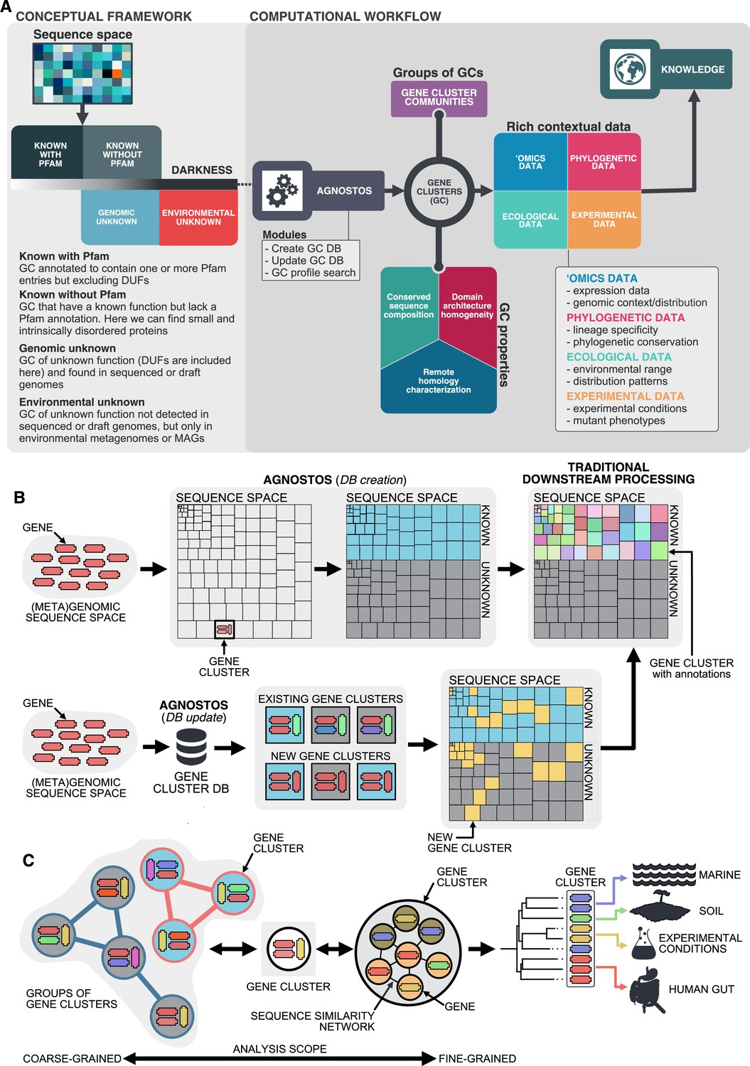
Conceptual framework to unify the known and unknown sequence space and integration of the framework in the current analytical workflows.
(A) Link between the conceptual framework and the computational workflow to partition the sequence space in the four conceptual categories. AGNOSTOS infers, validates and refines the GCs and combines them in gene cluster communities (GCCs). Then, it classifies them in one of the four conceptual categories based on their level of ‘darkness’. Finally, we add context to each GC based on several sources of information, providing a robust framework for generating hypotheses that can be used to augment experimental data. (B) The computational workflow provides two mechanisms to structure sequence space using GCs, de novo creation of the GCs (DB creation), or integrating the dataset in an existing GC database (DB update). The structured sequence space can then be plugged into traditional analytical workflows to annotate the genes within each GC of the known fraction. With AGNOSTOS, we provide the opportunity to integrate the unknown fraction into microbiome analyses easily. (C) The versatility of the GCs enables analyses at different scales depending on the scope of our experiments. We can group GCs in gene cluster communities based on their shared homologies to perform coarse-grained analyses. On the other hand, we can design fine-grained analyses using the relationships between the genes in a GC, that is detecting network modules in the GC inner sequence similarity network. Additionally, given that GCs are conserved across environments, organisms and experimental conditions give us access to an unprecedented amount of information to design and interpret experimental data.
Figure 2

Overview and validation of the workflow to aggregate GCs in communities.
(A) We inferred a gene cluster homology network using the results of an all-vs-all HMM gene cluster comparison with HHBLITS. The edges of the network are based on the HHblits-score/Aligned-columns. Communities are identified by an iterative screening of different MCL inflation parameters and evaluated using five different metrics that consider the inter- and intra-community properties. (B) Comparison of the number of GCs and GCCs for each of the functional categories. (C) Validation of the GCCs inference based on the environmental genes annotated as proteorhodopsins. Ribbons in the alluvial plot are genes, and each stacked bar corresponds (from left to right) to the (1) gene taxonomic classification at the domain level, (2) GC membership, (3) GCC membership and (4) MicRhoDE operational classification. (D) Validation of the GCCs inference based on ribosomal proteins based on standard and high-quality GCs.
Figure 3
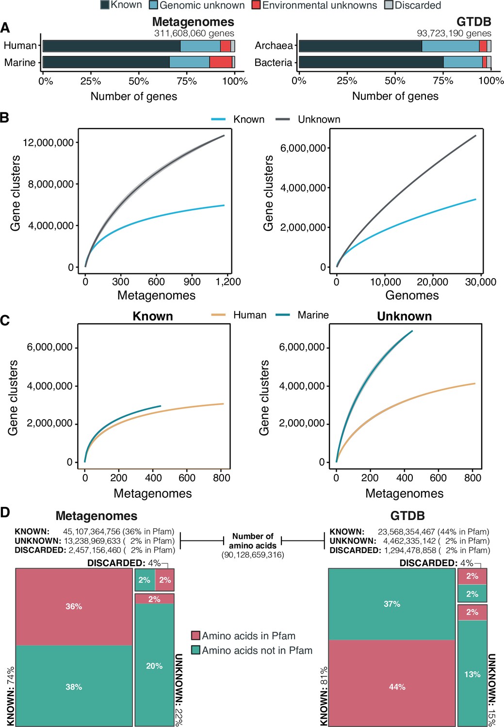
The extent of the known and unknown sequence space.
(A) Proportion of genes in the known and unknown. (B) Accumulation curves for the known and unknown sequence space at the GC- level for the metagenomic and genomic data. from TARA, MALASPINA, OSD2014 and HMP-I/II projects. (C) Collector curves comparing the human and marine biomes. Colored lines represented the mean of 1000 permutations and shaded in gray the standard deviation. Non-abundant singleton clusters were excluded from the accumulation curves calculation. (D) Amino acid distribution in the known and unknown sequence space. In all cases, the four categories have been simplified as known (K, KWP) and unknown (GU, EU).
Figure 4
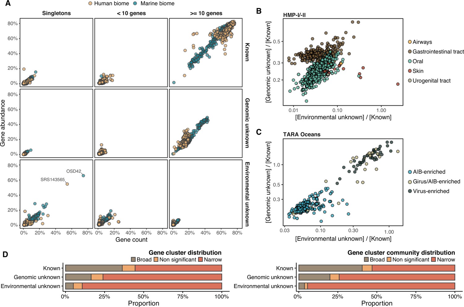
Distribution of the unknown sequence space in the human and marine metagenomes.
(A) Ratio between the proportion of the number of genes and their estimated abundances per cluster category and biome. Columns represented in the facet depicts three cluster categories based on the size of the clusters. (B) Relationship between the ratio of Genomic unknowns and Environmental unknowns in the HMP-I/II metagenomes. Gastrointestinal tract metagenomes are enriched in Genomic unknown sequences compared to the other body sites. (C) Relationship between the ratio of Genomic unknowns and Environmental unknowns in the TARA Oceans metagenomes. Girus- and virus-enriched metagenomes show a higher proportion of both unknown sequences (genomic and environmental) than the Archaea|Bacteria enriched fractions. (D) Environmental distribution of GCs and GCCs based on Levin’s niche breadth index. We obtained the significance values after generating 100 null gene cluster abundance matrices using the quasiswap algorithm.
Figure 5

Phylogenomic exploration of the unknown sequence space.
(A) Distribution of the lineage-specific GCs by taxonomic level. Lineage-specific unknown GCs are more abundant in the lower taxonomic levels (genus, species). (B) Phylogenetic conservation of the known and unknown sequence space in 27,372 bacterial genomes from GTDB_r86. We observe differences in the conservation between the known and the unknown sequence space for lineage- and non-lineage specific GCs (paired Wilcoxon rank-sum test; all p-values < 0.0001). (C) The majority of the lineage-specific clusters are part of the unknown sequence space, and only a small proportion was found in prophages present in the GTDB_r86 genomes. (D) Known and unknown sequence space of the 27,732 GTDB_r86 bacterial genomes grouped by bacterial phyla. Phyla are partitioned based on the ratio of known to unknown GCs and vice versa. Phyla enriched in MAGs have higher proportions in GCs of unknown function. Phyla with a high proportion of non-classified clusters (NC; discarded during the validation steps) tend to contain a small number of genomes. (E) The alluvial plot’s left side shows the uncharacterized (OM-RGC v2 GC) and characterized (OM-RGC v2) fraction of the gene catalog. The functional annotation is based on the eggNOG annotations provided by Salazar et al., 2019. The right side of the alluvial plot shows the new organization of the OM-RGC v2 sequence space based on the approach described in this study. The treemap in the right links the metagenomic and genomic space adding context to the unknown fraction of the OM-RGC v2.
Figure 6
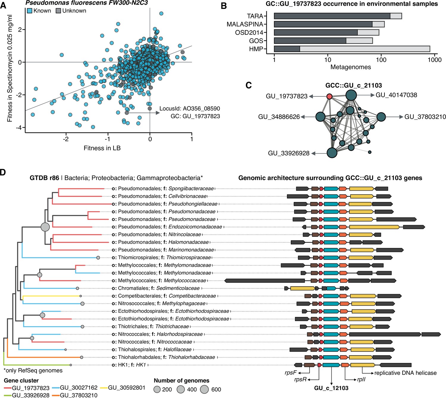
Augmenting experimental data with GCs of unknown function.
(A) We used the fitness values from the experiments from Price et al., 2018 to identify genes of unknown function that are important for fitness under certain experimental conditions. The selected gene belongs to the genomic unknown GC GU_19737823 and presents a strong phenotype (fitness = –3.1; t = –9.1) (B) Occurrence of GU_19737823 in the metagenomes used in this study. Darker bars depict the number of metagenomes where the GC is found. (C) GU_19737823 is a member of the GCC GU_c_21103. The network shows the relationships between the different GCs members of the gene cluster community GU_c_21103. The size of the node corresponds to the node degree of each GC. Edge thickness corresponds to the bitscore/column metric. Highlighted in red is GU_19737823. (D) We identified all the genes in the GTDB_r86 genomes that belong to the GCC GU_c_21103 and explored their genomic neighborhoods. GU_c_21103 members were constrained to the class Gammaproteobacteria, and GU_19737823 is mostly exclusive to the order Pseudomonadales. The gene order in the different genomes analyzed is highly conserved, finding GU_19737823 after the rpsF::rpsR operon and before rpll. rpsF and rpsR encode for the 30 S ribosomal protein S6 and 30 S ribosomal protein S18, respectively. The GTDB_r86 subtree only shows RefSeq genomes. Branch colors correspond to the different GCs found in GU_c_21103. The bubble plot depicts the number of genomes with a gene that belongs to GU_c_21103.
Appendix 1—figure 1
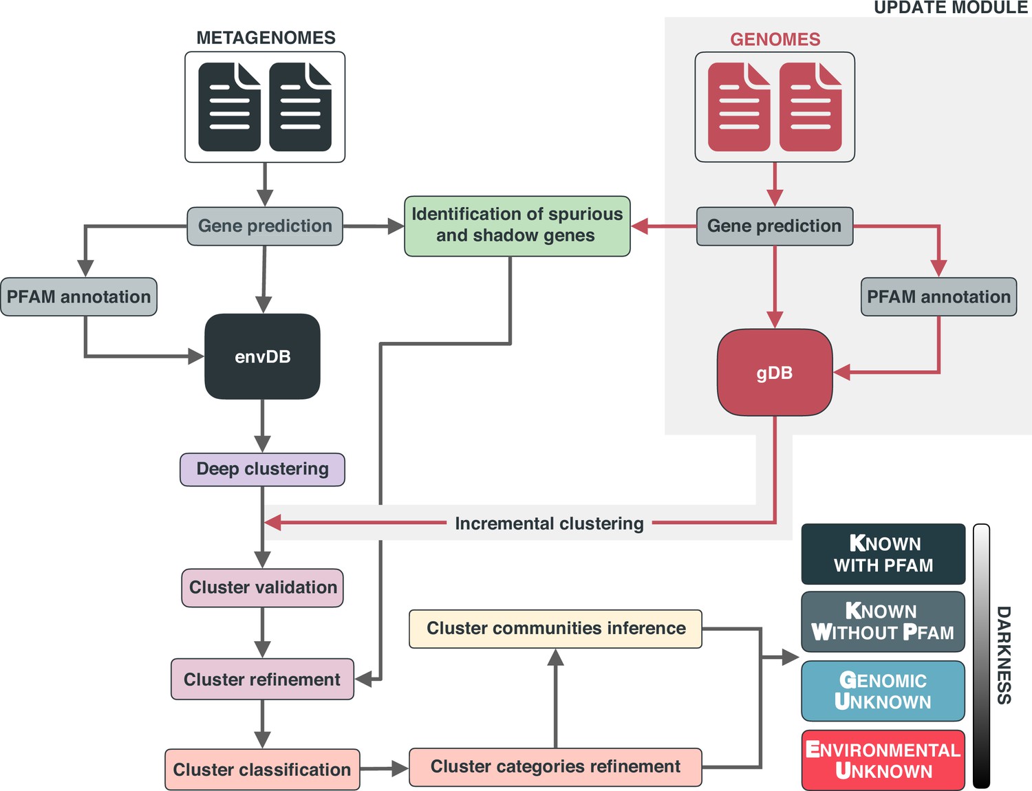
Overview of the workflow to partition the genomic and metagenomic sequence space between known and unknown.
The workflow performs gene prediction, gene clustering, gene clustering validation and refinement, GCC inference, and partitions the sequence space in the different known and unknown categories.
Appendix 1—figure 2

The diagram shows a schematic description of the number of genes and GCs that have been kept or discarded.
(A) We analyzed a dataset of 1749 metagenomes from marine and human environments and 28,941 genomes from the GTDB_r86 summing up to 415,971,742 genes. The composition of the genomic box ‘Other’ is described in Appendix Note 5. (B) GC overlap between the environmental and genomic datasets.
Appendix 1—figure 3
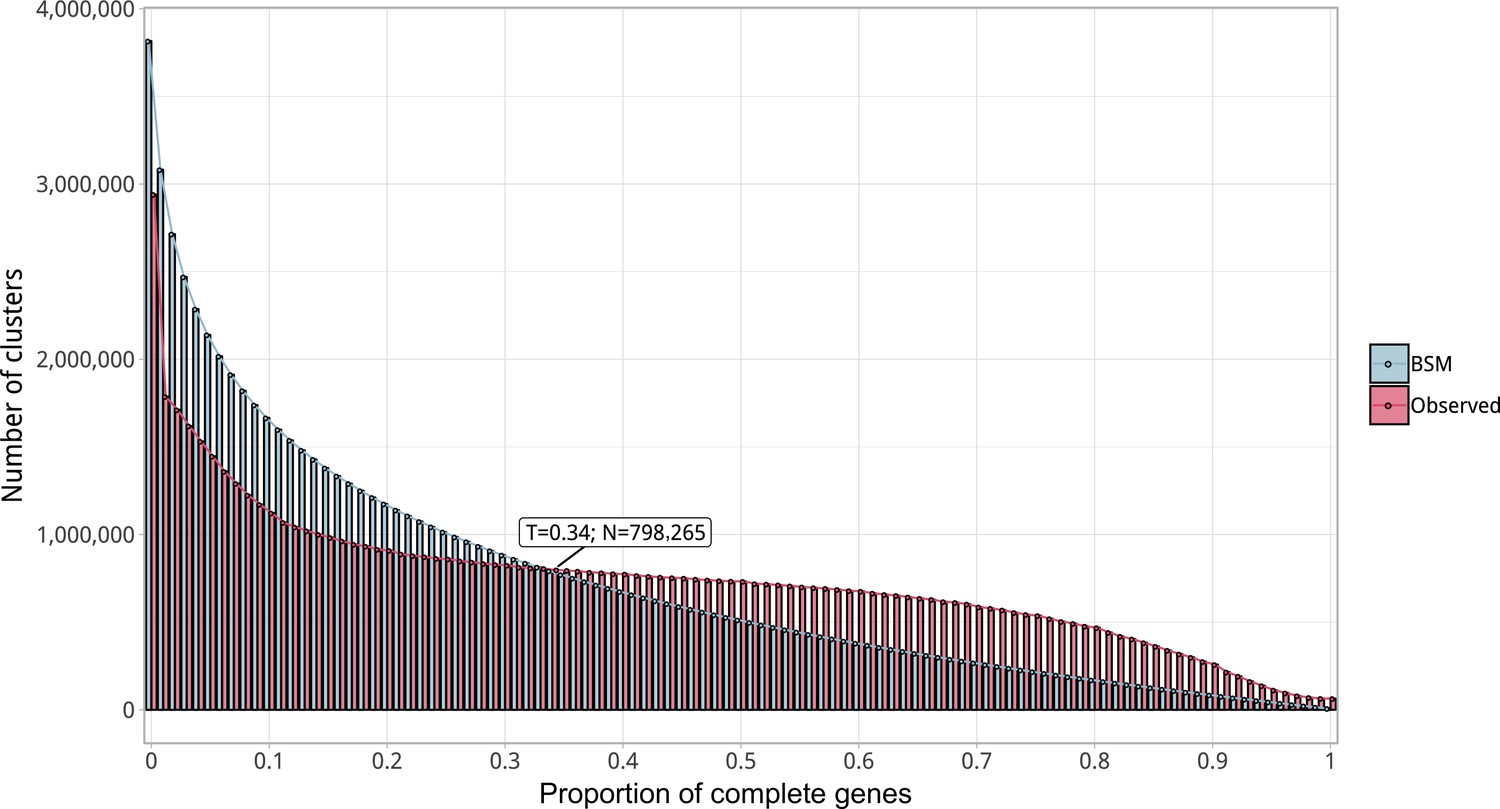
Proportion of complete genes per cluster.
Distribution of observed values compared with those generated by the Broken-stick model. The cut-off was determined at 34% complete genes per cluster.
Appendix 1—figure 4
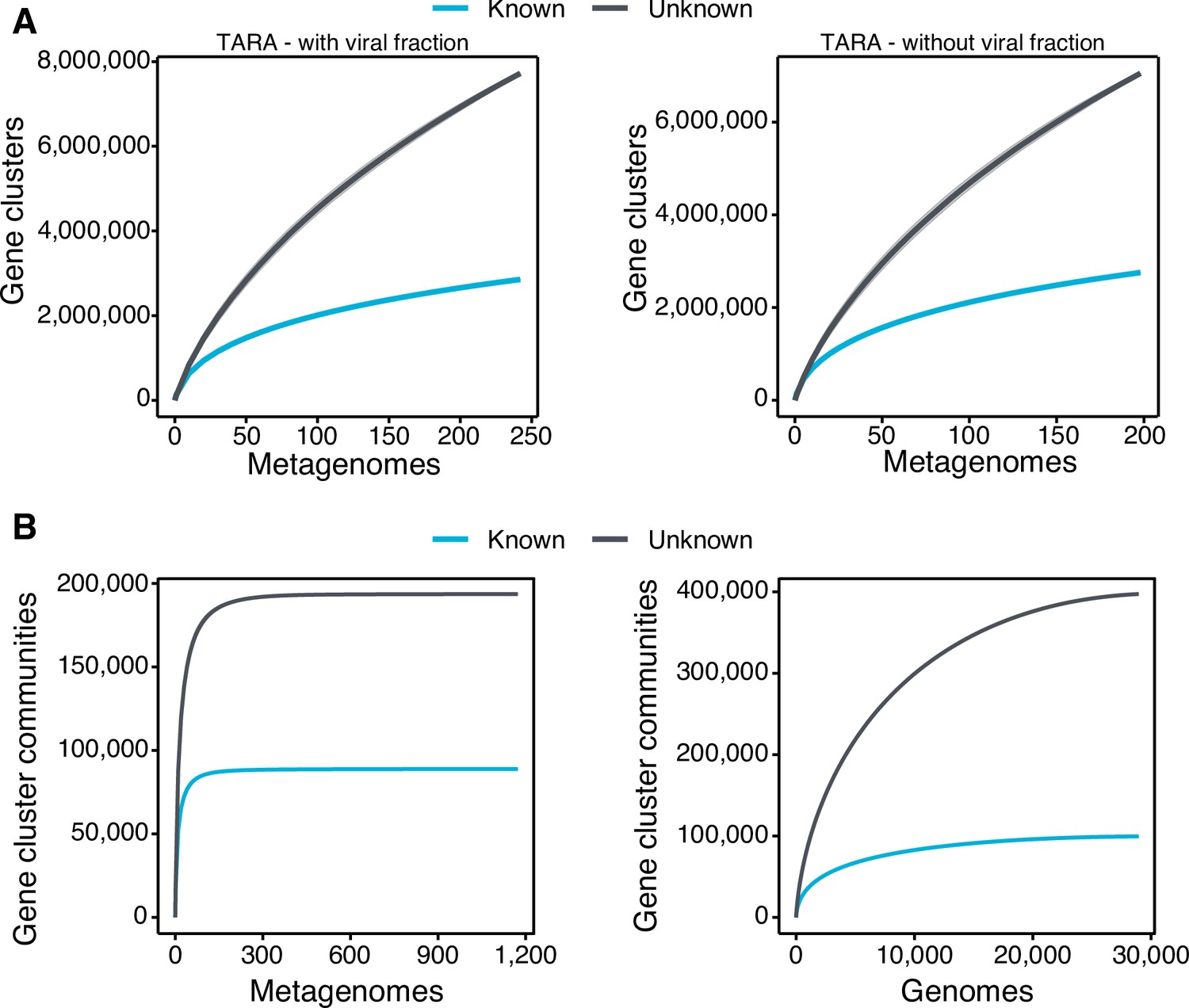
Collector curves for the known and unknown sequence space.
(A) Collector curves at the gene cluster level, for the TARA metagenomes, including the viral fraction (left) and excluding it (right) from the analysis. (B) Collector curves at gene cluster community level for the metagenomes from TARA, MALASPINA, and HMP-I/II projects (left) and the 28,941 GTDB genomes (right).
Appendix 1—figure 5

Collector curves for the known and unknown sequence space at the gene cluster level for (A) the metagenomes from TARA, MALASPINA and HMP-I/II projects, and for (B) the 28,941 GTDB genomes.
Singletons were excluded from the calculations.
Appendix 1—figure 6
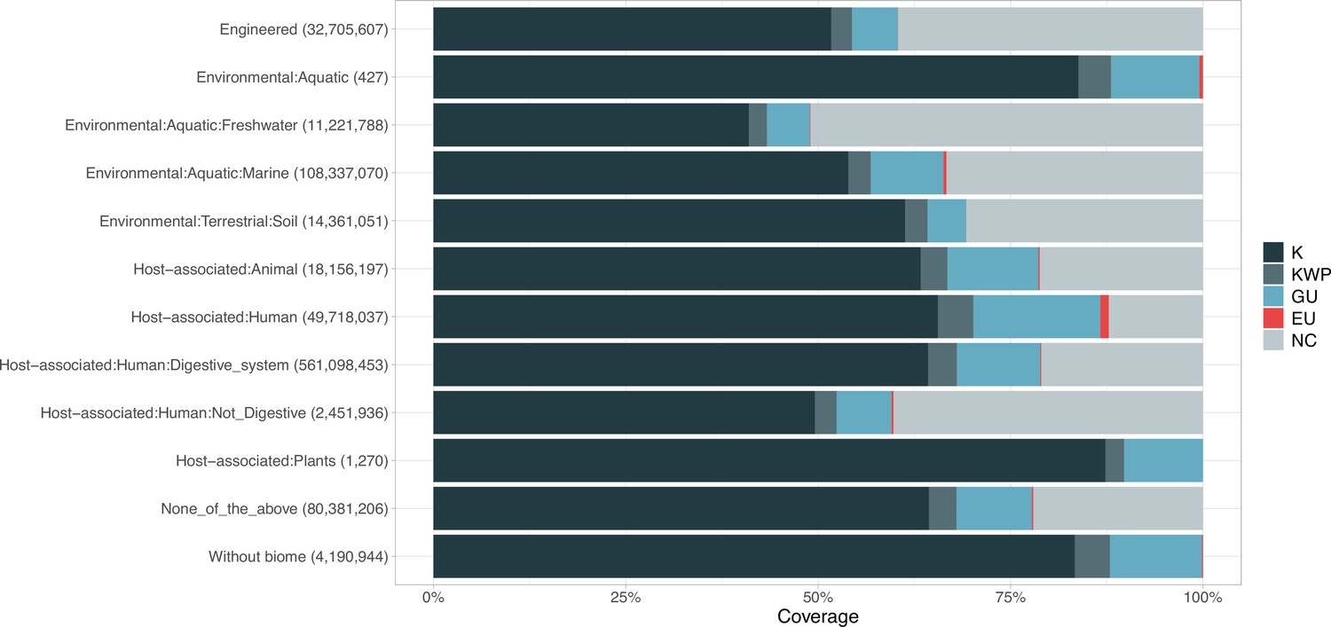
Proportion of gene cluster categories per biome.
On the y-axis are reported the 11 main biome categories indicated by MGnify and in parenthesis the total number of genes in each biome. The gray fraction represents the pool of genes from MGnify that were not found in our dataset.
Appendix 1—figure 7
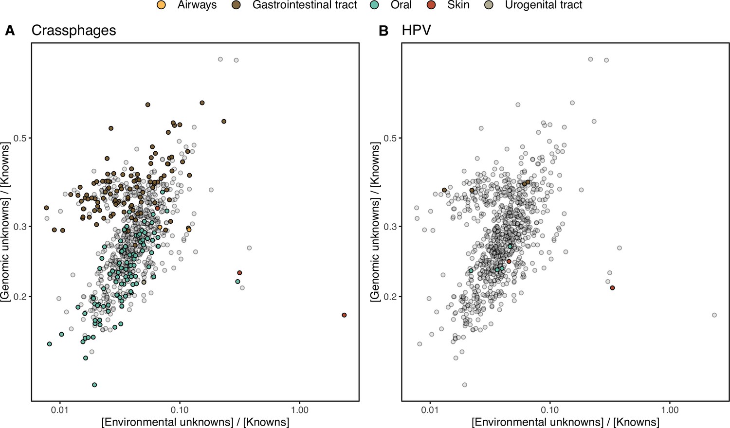
HMP outlier samples enriched in (A) crAssphages, and (B) papillomaviruses (HPV).
Appendix 1—figure 8

EggNOG annotations entropy within the GCs (A) and the GCCs (B).
The entropy was calculated using the function entropy.empirical() from the R package ‘entropy’, which estimates the Shannon entropy values based on the value empirical frequencies.
Appendix 3—figure 1
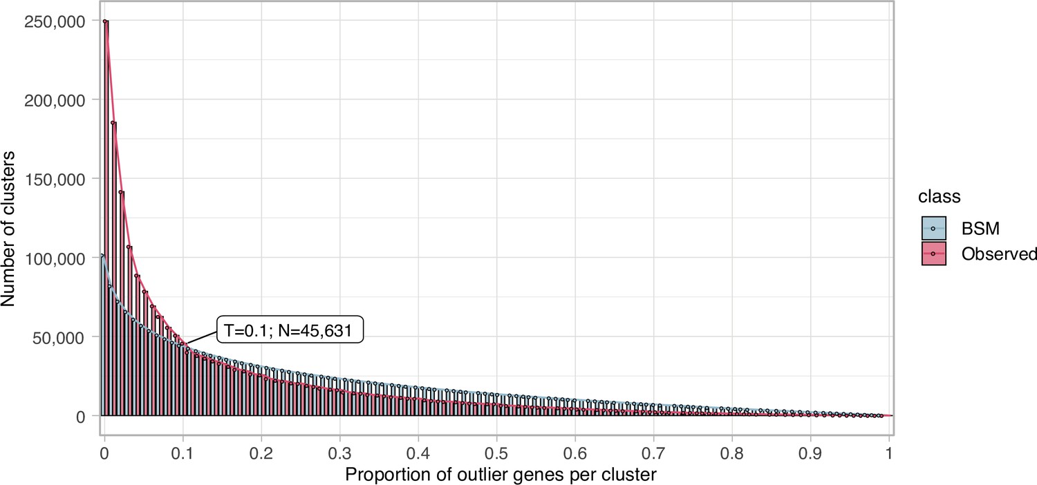
Proportion of outlier genes detected within each cluster MSA.
Distribution of observed values compared with those generated by the Broken-stick model. The cut-off was determined at 10% outlier genes per cluster.
Appendix 5—figure 1
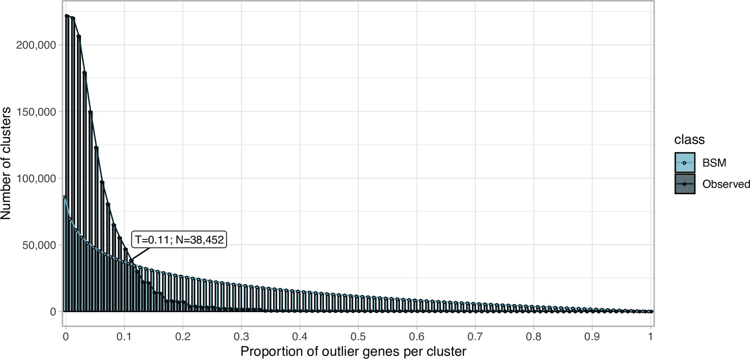
Proportion of outlier genomic genes identified within each cluster MSA.
Distribution of observed values compared with those of the Broken-stick model.
Appendix 5—figure 2
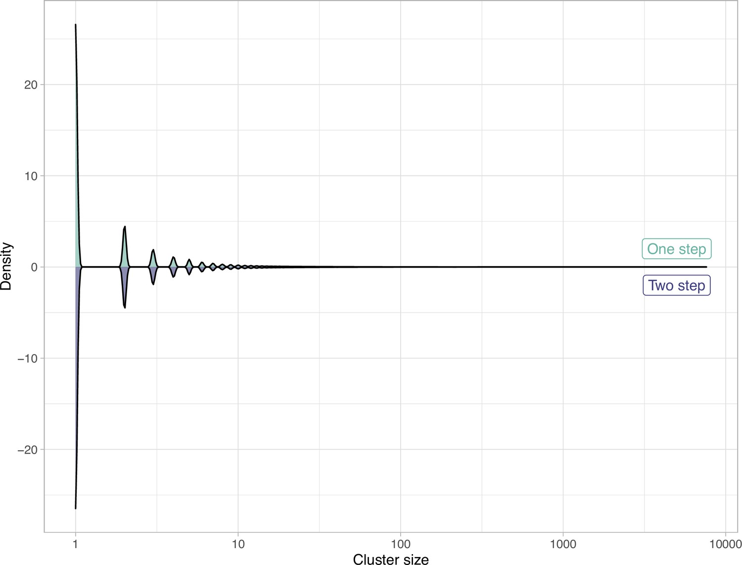
Comparison of the clustering results obtained with the one-step and two-step approach in terms of cluster composition.
Appendix 7—figure 1
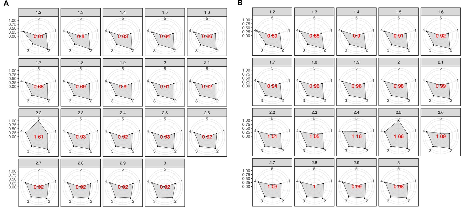
Radar plots used to determine the best MCL inflation value for the partitioning of the K into cluster components.
The plots were built using a combination of five variables: 1 = proportion of clusters with one component and 2 = proportion of clusters with more than one member, 3 = clan entropy (proportion of clusters with entropy = 0), 4 = intra HHblits-Score/Aligned-columns (normalized by the maximum value), and 5 = number of clusters (related to the non-redundant set of DAs). (A) Metagenomic dataset. (B) Genomic dataset.
Appendix 7—figure 2
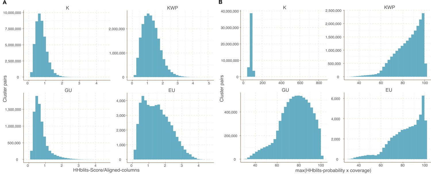
Cluster pairs distribution based on the metrics used to weight the gene cluster HMM-HMM homology network.
(A) HHblits-Score/Aligned-columns (Vanni et al., 2021). (B) maximum(HHblits-probability x coverage) (Méheust et al.).
Appendix 7—figure 3
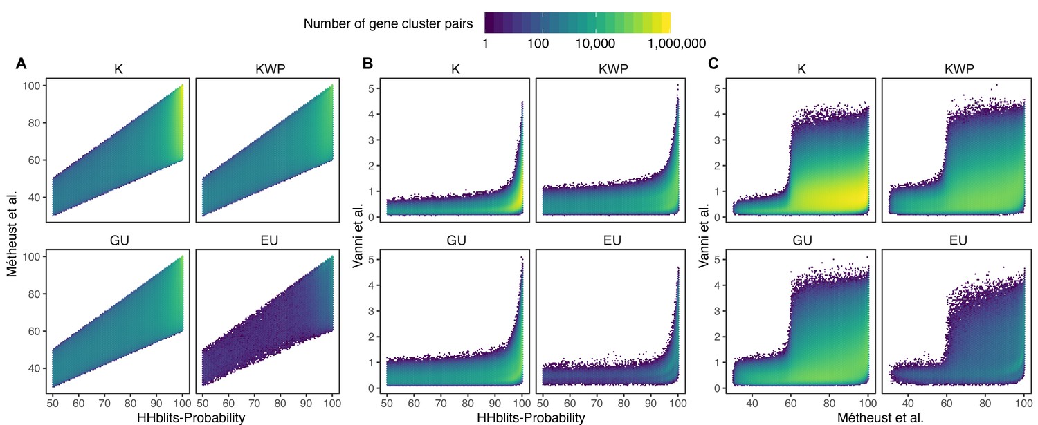
Determination of the edge-weight metrics for the GC HMM-HMM homology network.
We tested the metrics used in Méheust et al. and this paper (Vanni et al.). The correlations between metrics are shown per functional category. The metric used by Méheust et al. corresponds to the maximum(HHblits-probability x coverage). The metric applied in this manuscript is HHblits-Score/Aligned-columns. (A) Comparison between the metric of Méheust et al. and the HHblits-Probability. (B) Comparison between the metric used in this manuscript and the HHblits-Probability. (C) Comparison between the metric used in this manuscript and the metric of Méheust et al.
Appendix 7—figure 4

Agreement between the number of communities within ribosomal protein families between our approach and the one described in Méheust et al.
Appendix 9—figure 1
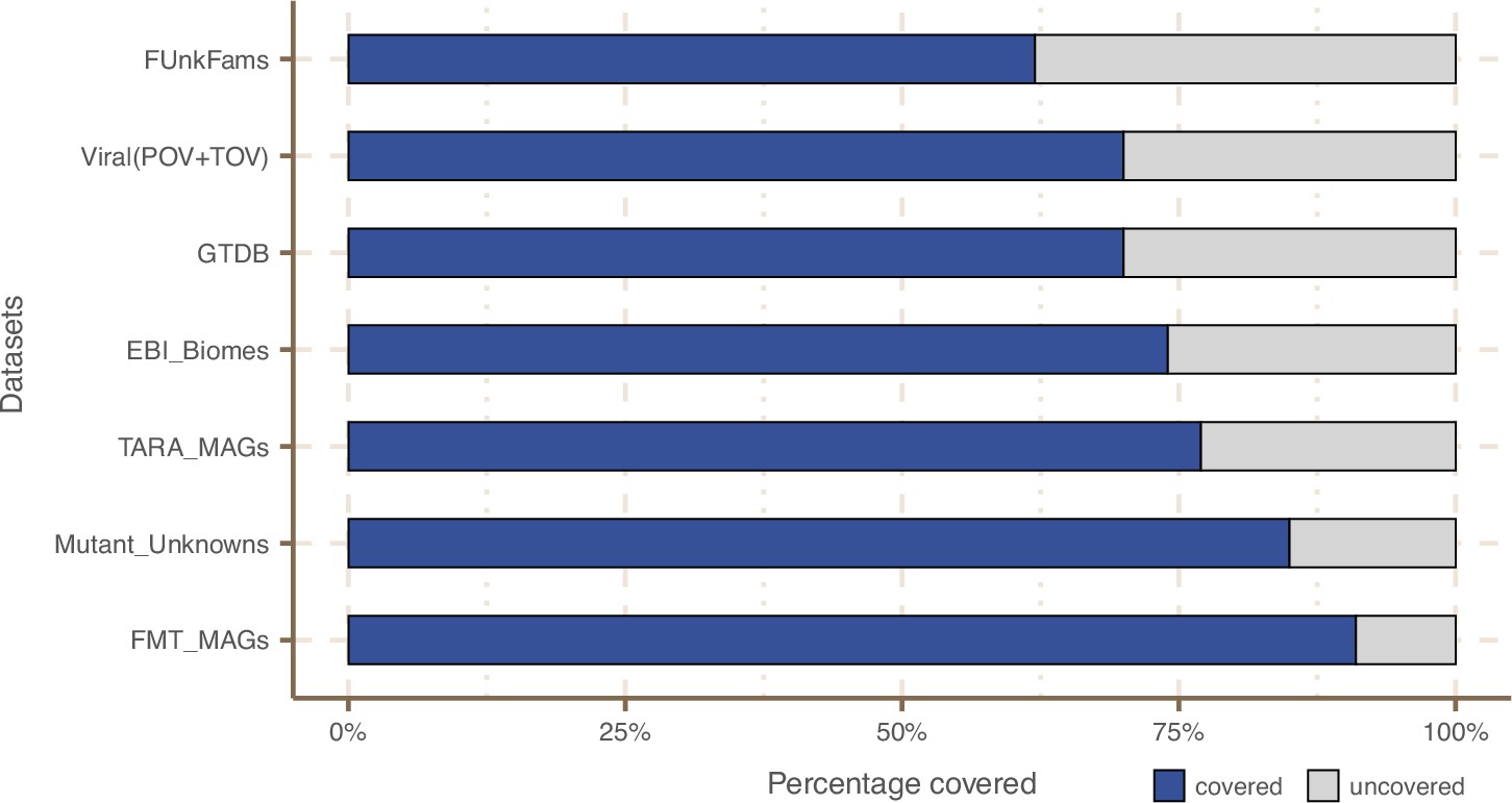
Coverage of external datasets.
The bar plot is showing the proportion of covered genes in each of the seven datasets that were screened against the metagenomic set of clusters’ HMM profiles.
Appendix 10—figure 1
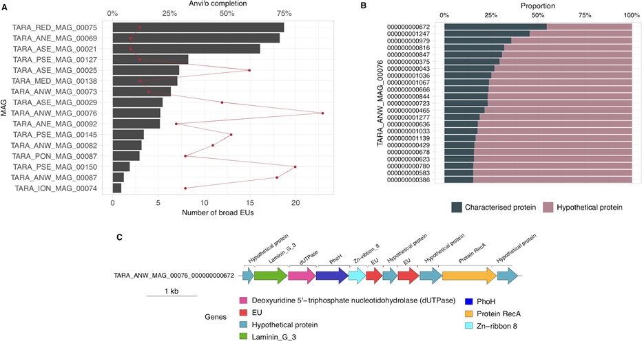
Broadly distributed EU mapping on TARA MAGs results.
(A) . Histogram of TARA MAG percent completeness (checkM). The red line represents the number of EU found in the MAGs. (B) Contigs from TARA MAGs TARA_ANW_MAG_00076 in descending order of highest proportion of non-hypothetical gene content. (C) EU communities in the context of a MAG contig. Contig genomic neighborhood around two potential EU communities.
Appendix 11—figure 1

Phylogenomic exploration of the unknown sequence space in Archaea.
(A) Distribution of the lineage-specific gene clusters by taxonomic level. Lineage-specific unknown gene clusters are more abundant at the lower taxonomic levels (genus, species). (B) Phylogenetic conservation of the known and unknown sequence space in 1,569 archaeal genomes from GTDB. We calculated the mean trait depth (add symbol D) with the consenTRAIT algorithm and the lineage specificity using the F1-score approach from Mendler et al., 2019. We observe differences in the conservation between the known and the unknown sequence space for lineage- and non-lineage-specific gene clusters (paired Wilcoxon rank-sum test; all P-values < 0.0001). (C) The majority of the lineage-specific clusters are part of the unknown sequence space, being a small proportion found in prophages present in the GTDB genomes. (D) Known and unknown sequence space of the 1,569 GTDB archaeal genomes grouped by archaeal phyla. Phyla are partitioned based on the ratio of known to unknown gene clusters and vice versa from the set of genomes. Phyla enriched in Metagenomic assembled genomes (MAGs) have a higher proportion in gene clusters of unknown function.
Appendix 12—figure 1
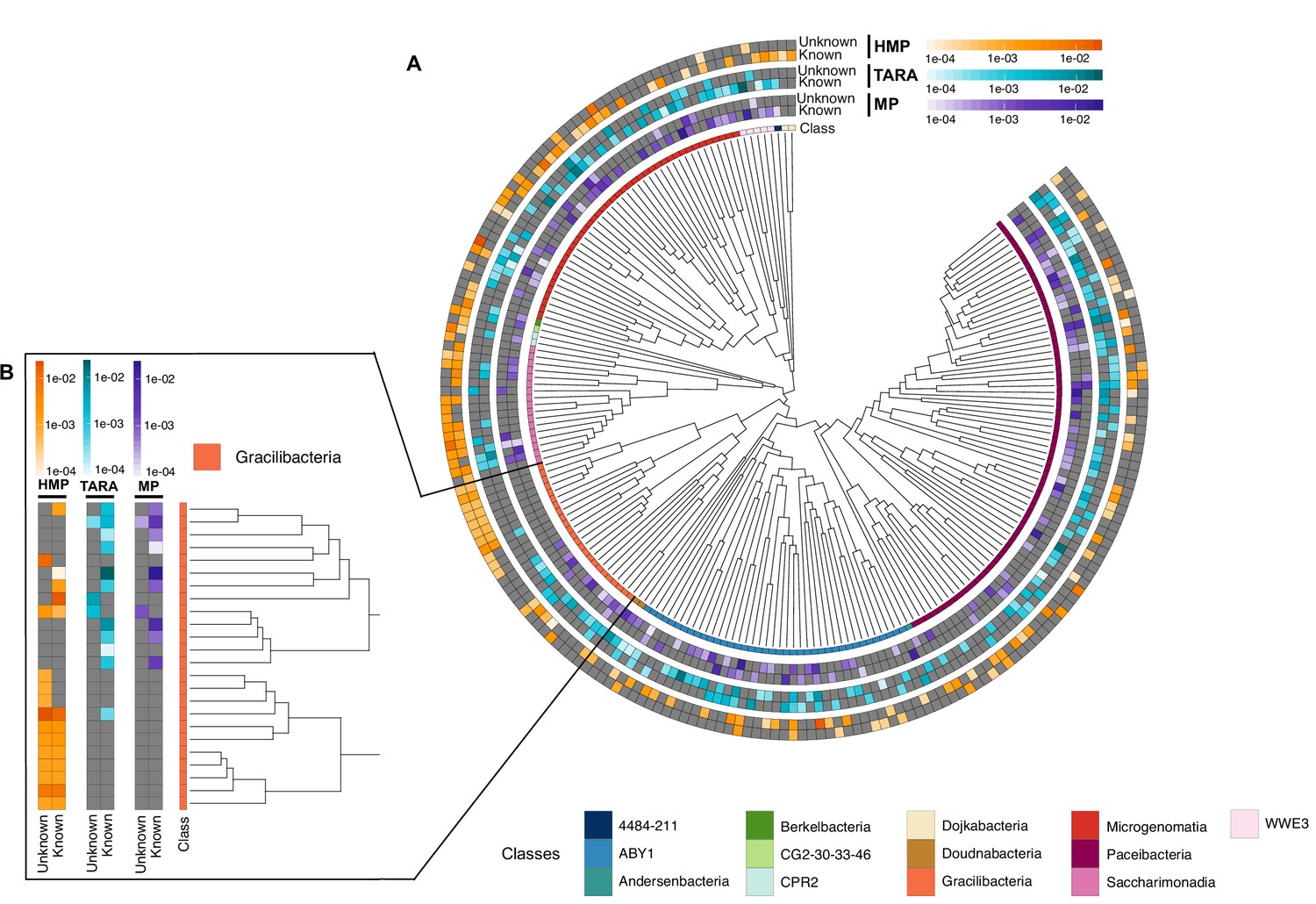
Cand Patescibacteria metagenomic lineage-specific clusters.
(A) Phylogenetic tree of Cand. Patescibacteria genera, colored by classes. The heatmaps around the tree show the proportion of lineage-specific gene clusters of knowns and unknowns in the metagenomes from TARA, Malaspina and the HMP. (B) Metagenomic lineage-specific clusters in the class of Gracilibacteria.
Tables
Key resources table
| Reagent type (species) or resource | Designation | Source or reference | Identifiers | Additional information |
|---|---|---|---|---|
| Software, algorithm | Snakemake | Snakemake | RRID: SCR_003475 | Workflow manager |
| Software, algorithm | Prodigal | Prodigal | RRID: SCR_021246 | Gene prediction |
| Software, algorithm | MMseqs2 | MMseqs2 | RRID: SCR_010277 | Sequence clustering and search |
| Software, algorithm | HHMER | HMMER | RRID: SCR_005305 | Sequence-Profile search |
| Software, algorithm | HHblits | HHblits | RRID: SCR_010277 | Profile-Profile search |
| Software, algorithm | PARASAIL | PARASAIL | RRID:SCR_021805 | Sequence alignment |
| Software, algorithm | FAMSA | FAMSA | RRID:SCR_021804 | Sequence alignment |
| Software, algorithm | LEON-BIS | LEON-BIS | RRID:SCR_021803 | Sequence alignment evaluation |
| Software, algorithm | OD-SEQ | OD-SEQ | Sequence alignment http://www.bioinf.ucd.ie/download/od-seq.tar.gz | |
| Software, algorithm | SEQKIT | SEQKIT | RRID: SCR_018926 | Fasta file manipulation |
| Software, algorithm | R | R | RRID: SCR_002394 | |
| Software, algorithm | HH-SUITE | HH-SUITE | RRID: SCR_016133 | |
| Software, algorithm | RAXML | RAXML | RRID: SCR_006086 | Phylogeny |
| Software, algorithm | PPLACER | PPLACER | RRID: SCR_004737 | Phylogeny |
| Software, algorithm | PAPARA | PAPARA | Sequence alignment https://cme.hits.org/exelixis/resource/download/software/papara_nt-2.5-static_x86_64.tar.gz | |
| Software, algorithm | Anvi’o | Anvi’o | RRID:SCR_021802 | Omics analysis and visualization https://merenlab.org/software/anvio |
| Software, algorithm | BWA mapper | BWA mapper | RRID: SCR_010910 | Sequence alignment |
| Software, algorithm | BEDTOOLS | BEDTOOLS | RRID: SCR_006646 | |
| Software, algorithm | PhageBoost | PhageBoost | https://github.com/ku-cbd/PhageBoost | |
| Software, algorithm | EGGNOG-mapper | EGGNOG-mapper | RRID: SCR_021165 |
Appendix 1—table 1
Number of metagenomic clusters and genes after the validation and refinement steps.
| Good-quality | Bad-quality | Total | |
|---|---|---|---|
| Clusters | 2,940,257 | 63,640 | 32,465,074 |
| Genes | 260,142,354 | 8,325,409 | 322,248,552 |
Appendix 1—table 2
MG +GTDB high-quality (HQ) subset of gene clusters (GCs).
| Category | HQ GCs | HQ genes | pHQ GCs | pHQ genes |
|---|---|---|---|---|
| K | 76,718 | 40,710,936 | 0.0145 | 0.120 |
| KWP | 16,922 | 1,733,599 | 0.00320 | 0.005132 |
| GU | 95,370 | 9,908,630 | 0.0180 | 0.0293 |
| EU | 14,207 | 477,625 | 0.00269 | 0.00141 |
| Total | 203,217 | 52,830,790 | 0.0384 | 0.1562 |
Appendix 1—table 3
Mean proportion of complete genes per cluster in the four functional categories.
| K | KWP | GU | EU | |
|---|---|---|---|---|
| Mean percentage of complete genes | 0.50 | 0.22 | 0.68 | 0.70 |
Appendix 1—table 4
KWP high-quality gene clusters (GCs) distribution in the COG groups.
(Full table in Supplementary file 1A).
| COG group | Number of GCs | Proportion of GCs |
|---|---|---|
| CELLULAR PROCESSES AND SIGNALING | 2292 | 0.135 |
| INFORMATION STORAGE AND PROCESSING | 1582 | 0.0935 |
| METABOLISM | 1679 | 0.0992 |
| POORLY CHARACTERIZED | 2899 | 0.171 |
| NC | 8470 | 0.501 |
Appendix 1—table 5
Environmental (metagenomic) dataset description.
| (A) Number of samples and sites per metagenomic project. | ||||
|---|---|---|---|---|
| Dataset | Reference | Samples | Sites | Contigs |
| TARA | Sunagawa et al., 2015 | 242 | 141 | 62,404,654 |
| Malaspina | Duarte, 2015 | 116 | 30 | 9,330,293 |
| OSD | Kopf et al., 2015 | 145 | 139 | 4,127,095 |
| HMP | Lloyd-Price et al., 2017 | 1,246 | 18 | 80,560,927 |
| Dataset | Reference | Samples | Sites | Reads |
| GOS | Rusch et al., 2007 | 80 | 70 | 12,672,518 |
| (B) Number of predicted genes per completeness category. | ||||
| Total | "00" | "10" | "01" | "11" |
| 322,248,552 | 118,717,690 | 106,031,163 | 102,966,482 | 75,694,123 |
-
Note: "00" = complete, both start and stop codon identified. "01" = right boundary incomplete. "10" = left boundary incomplete. "11" = both left and right edges incomplete.
Appendix 1—table 6
Summary of the number of EU clusters based on their presence in MAGs and their environmental distribution, obtained with the Levin’s Niche Breadth index.
| Total clusters | Broad | Narrow | Non-significant | |
|---|---|---|---|---|
| Total EU | 204,031 | 471 | 8421 | 195,079 |
| EU in MAGs | 55,520 | 88 | 316 | 55,116 |
| EU not in MAGs | 148,511 (73%) | 383 (81%) | 8105 (96%) | 140,023 (72%) |
Appendix 1—table 7
Number of lineage-specific gene clusters of unknown function at different taxonomic levels within the Cand.
Patescibacteria phylum.
| Taxonomic level | Number of clusters |
|---|---|
| Phylum | 2 |
| Class | 6 |
| Order | 104 |
| Family | 1456 |
| Genus | 6987 |
| Species | 45,788 |
Appendix 1—table 8
Shannon entropy values for the eggNOG annotations within the gene clusters.
| Min. | 1st qu. | Median | Mean | 3rd qu. | Max. | |
|---|---|---|---|---|---|---|
| Entropy per GC | 0.000 | 0.000 | 0.000 | 0.105 | 0.000 | 3.729 |
Appendix 1—table 9
Shannon entropy values for the eggNOG annotations within the gene clusters communities.
| Min. | 1st qu. | Median | Mean | 3rd qu. | Max. | |
|---|---|---|---|---|---|---|
| Entropy per GCC | 0.000 | 0.000 | 0.000 | 0.285 | 0.400 | 3.721 |
Appendix 2—table 1
Singletons and small GCs Pfam annotations.
| Total | Annotated | Not annotated | |
|---|---|---|---|
| Singletons | 19,911,324 | 934,548 | 18,976,776 |
| Small GCs | 9,549,853 | 1,028,076 | 8,521,777 |
Appendix 2—table 2
Number of singletons and small GCs per functional category.
| K | KWP | GU | EU | |
|---|---|---|---|---|
| Singletons | 852,413 | 3,505,161 | 2,763,476 | 12,790,274 |
| Small GCs | 946,112 | 2,213,654 | 2,744,262 | 3,645,825 |
Appendix 3—table 1
Number of spurious, shadow and outlier genes in the metagenomic clusters.
| Gene category | Clusters ≥ 10 genes | Clusters < 10 genes | Singletons |
|---|---|---|---|
| Spurious | 44,205 | 6784 | 2,335 |
| Shadow | 289,258 | 144,571 | 177,126 |
| Outliers | 3,118,850 | - | - |
Appendix 3—table 2
Metagenomic gene cluster validation results.
| (A) Evaluation of cluster sequence composition. | |||
|---|---|---|---|
| Pre-Compos. validation | good quality | bad quality | |
| Clusters | 3,003,897 | 2,958,266 | 45,631 |
| Genes | 268,467,763 | 266,268,638 | 2,199,125 |
| (B) Evaluation of cluster Pfam functional annotations. | |||
| Pre-Funct. validation | Funct. good | Funct. bad | |
| Clusters | 1,015,924 | 1,004,166 | 11,758 |
| Genes | 181,433,541 | 178,167,583 | 3,246,002 |
Appendix 3—table 3
Steps: Step I - Removing of the "bad clusters".
Step II - Removing of the "shadow clusters". Step III - Removing single spurious, shadow or outlier genes.
| (A) Number of clusters in each step of the cluster refinement. | ||||
|---|---|---|---|---|
| Step I | Step II | Step III | Refined | |
| Clusters | 3,003,897 | 2,946,845 | 2,940,593 | 2,940,257 |
| Removed | –57,052 | –6,252 | –336 | |
| (B) Number of genes in each step of the cluster refinement. | ||||
| Step I | Step II | Step III | Refined | |
| Genes | 268,467,763 | 263,022,636 | 262,851,348 | 260,142,354 |
| Removed | –5,445,127 | –171,288 | –2,708,994 | |
Appendix 4—table 1
Metagenomic gene clusters classification steps.
| (A) Results from the search against the UniRef90 database | ||
|---|---|---|
| Search vs UniRef90 | Hits | No-hits |
| Initial clusters:1,946,737 | 1,581,115 | 365,622 |
| Characterized | Hypothetical | |
| 749,439 | 831,676 | |
| (B) Results from the search against the and the NCBI nr databases | ||
| Search vs NCBI nr | Hits | No-hits |
| Initial clusters: 365,622 | 20,277 | 345,345 |
| Characterized | Hypothetical | |
| 4,279 | 15,998 | |
| (C) Classification of the Pfam annotated GCs based on the consensus DAs. | ||
| Consensus DA analysis | Annotated to DKF DAs | Annotated to DUF DAs |
| Initial clusters: 993,520 | 912,551 | 80,969 |
Appendix 4—table 2
Metagenomic GC remote homology refinement steps.
| K | KWP | GU | EU | |
|---|---|---|---|---|
| Initial GCs | 912,551 | 753,718 | 928,643 | 345,345 |
| EU refinement | - | + 38,333 | + 171,183 | –209,516 |
| Post-EU refinement | 912,551 | 792,051 | 1,099,826 | 135,829 |
| KWP refinement | + 137,615 | –159,598 | + 21,983 | - |
| Refined GCs | 1,050,166 | 632,453 | 1,121,809 | 135,829 |
Appendix 5—table 1
GTDB integration in the metagenomic dataset.
| Metagenomic | Shared | Genomic | Total | |
|---|---|---|---|---|
| GCs | 30,301,693 | 2,163,381 | 7,958,475 | 40,423,549 |
| Genes | 199,693,614 | 190,001,314 | 26,276,814 | 415,971,742 |
Appendix 5—table 2
Genomic GC validation results.
| (A) Evaluation of cluster sequence composition. | |||
|---|---|---|---|
| Pre-Compos. validation | good quality | bad quality | |
| GCs | 2,400,037 | 2,361,585 | 38,452 |
| Genes | 20,718,376 | 20,364,454 | 353,922 |
| (B) Evaluation of Pfam functional annotations. | |||
| Pre-Funct. validation | good quality | bad quality | |
| GCs | 556,834 | 542,410 | 14,424 |
| Genes | 10,091,203 | 9,865,550 | 225,653 |
| (C) Combined cluster validation results. | |||
| Pre-validation | good quality | bad quality | |
| GCs | 2,400,037 | 2,347,502 | 52,535 |
| Genes | 20,718,376 | 20,141,636 | 576,740 |
Appendix 5—table 3
Spurious, shadow, and outlier genes in the genomic GCs.
| Gene category | GCs ≥ 2 genes | Singletons |
|---|---|---|
| Spurious | 3,252 | 1,312 |
| Shadow | 223,535 | 125,262 |
| Outliers | 449,080 | - |
Appendix 5—table 4
Non-annotated genomic GC classification.
| (A) Results from the search against the UniRef90 database. | |||
|---|---|---|---|
| Search vs UniRef90 | Hits | No-hits | |
| Initial GCs: 1,816,999 | 1,570,094 | 246,905 | |
| Characterized | Hypothetical | ||
| 304,004 | 1,266,090 | ||
| (B) Results from the search against the NCBI nr database. | |||
| Search vs NCBI nr | Hits | No-hits | |
| Initial GCs: 246,905 | 28,704 | 218,201 | |
| Characterized | Hypothetical | ||
| 1,280 | 27,424 | ||
| (C) Classification of the Pfam annotated GCs based on the consensus DAs. | |||
| Consensus DA analysis | DKF DAs | DUF DAs | |
| Initial GCs: 993,520 | 912,551 | 65,688 | |
Appendix 5—table 5
Genomic GC remote homology refinement and final genomic GC dataset.
| (A) Remote-homology refinement steps. | |||||
|---|---|---|---|---|---|
| K | KWP | GU | EU | ||
| Initial GCs | 464,815 | 305,284 | 1,359,202 | 218,201 | |
| EU refinement | - | + 5,704 | + 144,295 | –149,999 | |
| Post-EU refinement | 464,815 | 310,988 | 1,503,497 | 68,202 | |
| KWP refinement | + 152,529 | –174,582 | + 22,053 | - | |
| Refined GCs | 617,344 | 136,406 | 1,525,550 | 68,202 | |
| (B) Genomic GC refined dataset. | |||||
| K | KWP | GU | EU | Total | |
| Genes | 9,997,529 | 663,107 | 9,305,621 | 175,379 | 20,141,636 |
| GCs | 617,344 | 136,406 | 1,525,550 | 68,202 | 2,347,502 |
Appendix 5—table 6
Genomic high quality (HQ) GCs.
| Category | HQ GCs | HQ genes | pHQ GCs | pHQ genes |
|---|---|---|---|---|
| K | 12,202 | 25,105,156 | 0.0198 | 0.0096 |
| KWP | 4,019 | 1,349,165 | 0.0295 | 0.0214 |
| GU | 12,699 | 8,403,393 | 0.0083 | 0.0062 |
| EU | 438 | 471,820 | 0.0064 | 0.0074 |
Appendix 5—table 7
MG +GTDB seed database.
Integrated number of genes and GCs per category.
| K | KWP | GU | EU | Total | |
|---|---|---|---|---|---|
| Genes | 230,641,76 | 32,754,365 | 68,509,335 | 3,534,207 | 335,439,673 |
| GCs | 1,667,510 | 768,859 | 2,647,359 | 204,031 | 5,287,759 |
Appendix 5—table 8
Overview of genomic genes found homologous to metagenomic genes.
| Total | In MG good-quality GCs | In MG small GCs | In MG singletons | In MG bad-quality GCs | |
|---|---|---|---|---|---|
| Genes | 67,446,376 | 55,155,683 | 7,010,987 | 3,700,844 | 1,578,862 |
Appendix 5—table 9
Comparison of one-step and two-step clustering results in numbers.
| Approach | Total number of gene clusters | Of which singletons |
|---|---|---|
| One-step | 5,430,780 | 3,770,230 |
| Two-step | 5,462,006 | 3,779,961 |
Appendix 6—table 1
Number of MG +GTDB GCs annotated to the DPD per functional category.
| K | KWP | GU | EU |
|---|---|---|---|
| 374,555 | 8,874 | 22,135 | 0 |
Appendix 7—table 1
Number of gene clusters, cluster communities, and reduction rate shown by functional category.
| (A) Metagenomic dataset (MG) | |||||
|---|---|---|---|---|---|
| K | KWP | GU | EU | Total | |
| Clusters | 1,050,166 | 632,453 | 1,121,809 | 135,829 | 2,940,257 |
| Communities | 24,181 | 64,938 | 146,100 | 48,095 | 283,314 |
| Reduction (%) | 97.7 | 89.73 | 86.98 | 64.59 | 90.36 |
| (B) Genomic dataset (GTDB) | |||||
| K | KWP | GU | EU | Total | |
| Clusters | 617,344 | 136,406 | 1,525,550 | 68,202 | 2,347,502 |
| Communities | 52,360 | 47,203 | 339,468 | 57,899 | 496,930 |
| Reduction (%) | 91.52 | 65.39 | 77.75 | 15.11 | 79.30 |
Appendix 7—table 2
Measures of similarity between the community inference approach proposed in this paper, the one used in Méheust et al and the "ground truth" represented by the ribosomal protein families.
| Vanni et al. vs meheust et al. | Vanni et al. vs ribosomal families | Meheust et al. vs ribosomal families | |
|---|---|---|---|
| ARI | 0.915 | 0.944 | 0.906 |
| AMI | 0.928 | 0.916 | 0.878 |
| NVI | 0.101 | 0.0858 | 0.124 |
| NID | 0.0717 | 0.0841 | 0.122 |
| NMI | 0.928 | 0.916 | 0.878 |
-
Note: ARI = Adjusted Rand Index; AMI = Adjusted Mutual Information; NVI = Normalized Variation Information; NID = Normalized Information Distance; NMI = Normalized Mutual Information.
Appendix 8—table 1
Number of genomic singletons per functional category.
| K | KWP | GU | EU | |
|---|---|---|---|---|
| Genes | 473,460 | 896,127 | 2,528,370 | 1,660,481 |
Appendix 8—table 2
Minimum slope values for the collector curves.
| (A )Excluding singletons. In parenthesis, the number of genomes or metagenomes for the first occurrence of slope <1 | ||||||
|---|---|---|---|---|---|---|
| Gene Clusters | Gene cluster Communities | |||||
| metaG | GTDB | metaG | GTDB | |||
| Known | 209.235 | 6.556 | 0.1344 (440) | 0.07 (15,120) | ||
| Unknown | 374.5147 | 5.851 | 0.1375 (600) | 0.621 (27,690) | ||
| (B) Including singletons (with a mode abundance in the samples of 8.36). | ||||||
| Gene Clusters | ||||||
| metaG | GTDB | |||||
| Known | 1329.489 | 66.063 | ||||
| Unknown | 4843.570 | 158.891 | ||||
Appendix 9—table 1
Re-classification of the unknowns identified in Wyman et al and Price et al.
| Study | Original unknown set | Covered fraction | Found as known | Found as unknown |
|---|---|---|---|---|
| Wyman et al. | 61,970 | 38,174 | 12,366 | 25,808 |
| Price et al. | 49,736 | 33,016 | 21,967 | 11,049 |
Appendix 12—table 1
Number of lineage-specific clusters within the Cand.
Patescibacteria phylum, at different taxonomic levels, subdivided by cluster categories.
| Taxonomic level | K | KWP | GU | EU |
|---|---|---|---|---|
| Phylum | 1 | 0 | 2 | 0 |
| Class | 11 | 0 | 6 | 0 |
| Order | 41 | 1 | 104 | 0 |
| Family | 452 | 9 | 1,443 | 13 |
| Genus | 625 | 98 | 6,649 | 338 |
| Species | 4,116 | 818 | 42,710 | 3,078 |
Additional files
-
Supplementary file 1
Supplementary tables.
(a) KWP high-quality gene clusters (GCs) distribution in the COG groups. (b) Proportion of genes in each cluster category, and Pfam amino acids coverage per cluster category. (c) List of HMP outlier samples. (d) Number of phylogenetic conserved and lineage-specific gene clusters (GCs) in the GTDB bacterial phylogeny. (e) Clusters in the GU community GU_c_21103. (f) List of filtered samples used for the metagenomic analyses. (g) List of terms commonly used to define proteins of unknown function in public databases. (h) Sequence similarity values between viral genes and Needham et al. viral PRs. (i) Number of phylogenetic conserved and lineage-specific GCs in the GTDB archaeal phylogeny.
- https://cdn.elifesciences.org/articles/67667/elife-67667-supp1-v2.xlsx
-
Supplementary file 2
Supplementary tables describing general cluster properties.
(a) Overall properties for the GCs of the integrated dataset (MG + GTDB). (b) Statistics for the integrated dataset (MG+GTDB). (c) Taxonomic variation within each gene cluster category. (d) Statistics for the metagenomic dataset. (e) Statistics for the genomic dataset.
- https://cdn.elifesciences.org/articles/67667/elife-67667-supp2-v2.xlsx
-
Transparent reporting form
- https://cdn.elifesciences.org/articles/67667/elife-67667-transrepform1-v2.pdf
Download links
A two-part list of links to download the article, or parts of the article, in various formats.
Downloads (link to download the article as PDF)
Open citations (links to open the citations from this article in various online reference manager services)
Cite this article (links to download the citations from this article in formats compatible with various reference manager tools)
Unifying the known and unknown microbial coding sequence space
eLife 11:e67667.
https://doi.org/10.7554/eLife.67667


