Cortical magnification in human visual cortex parallels task performance around the visual field
- Department of Psychology, New York University, United States
- Center for Neural Sciences, New York University, United States
Figures
Figure 1
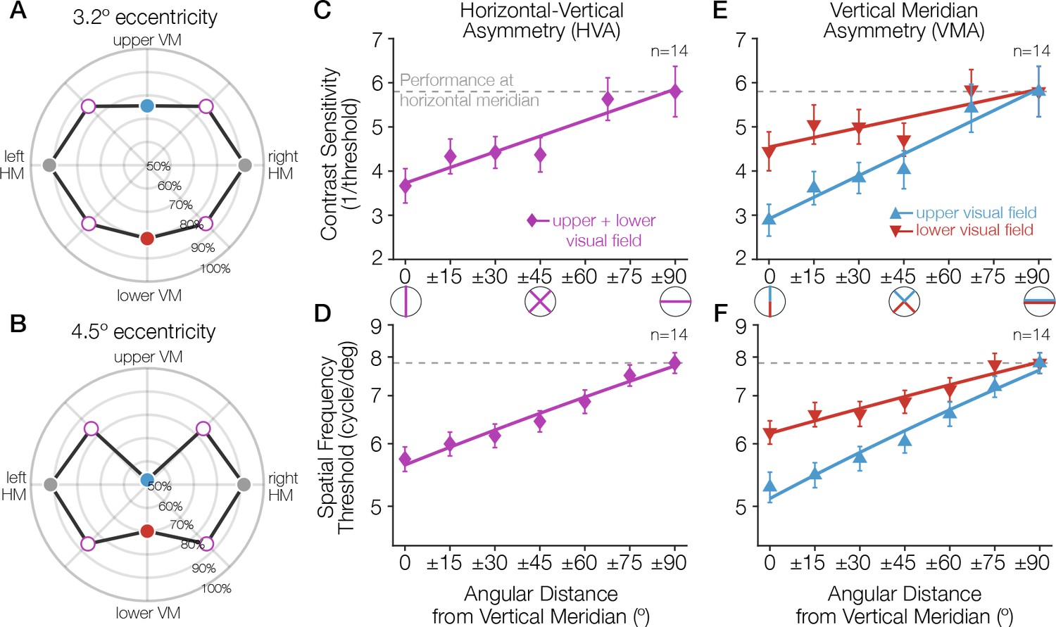
Task performance around the visual field.
(A, B) Performance for a Gabor-orientation discrimination task is shown in polar coordinates. The plotted angle indicates the polar angle of the tested stimulus location, and the distance from the origin indicates the performance (percent correct) at that polar angle. The origin indicates chance performance. Gabor patches were presented at either (A) 3.2° or (B) 4.5° of eccentricity, with a spatial frequency of 10 and 12 cycles/deg, respectively. The HVA and VMA are evident in both plots and the asymmetries are more pronounced at the farther eccentricity (Carrasco et al., 2001). (C–E) As the angular distance from the vertical meridian increases, averaged across upper and lower, performance gradually improves, approaching the performance level at the horizontal (C, D), and the difference in performance between the upper and lower hemifields reduces (E, F). These gradual changes around the visual field have been observed for contrast sensitivity (Abrams et al., 2012) (C, E; at 6° eccentricity) and acuity limit (Barbot et al., 2021) (D, F; at 10° eccentricity). Each data point corresponds to the average contrast sensitivity (or spatial frequency threshold) at a given angular location, with ±1 SEM across observers. Spatial frequency was measured as the point at which orientation discrimination performance dropped to halfway between ceiling and chance performance. Redrawn using data from Carrasco et al., 2001; Abrams et al., 2012 and Barbot et al., 2021. HVA, horizontal-vertical asymmetry; VMA, vertical meridian asymmetry.
Figure 2 with 1 supplement
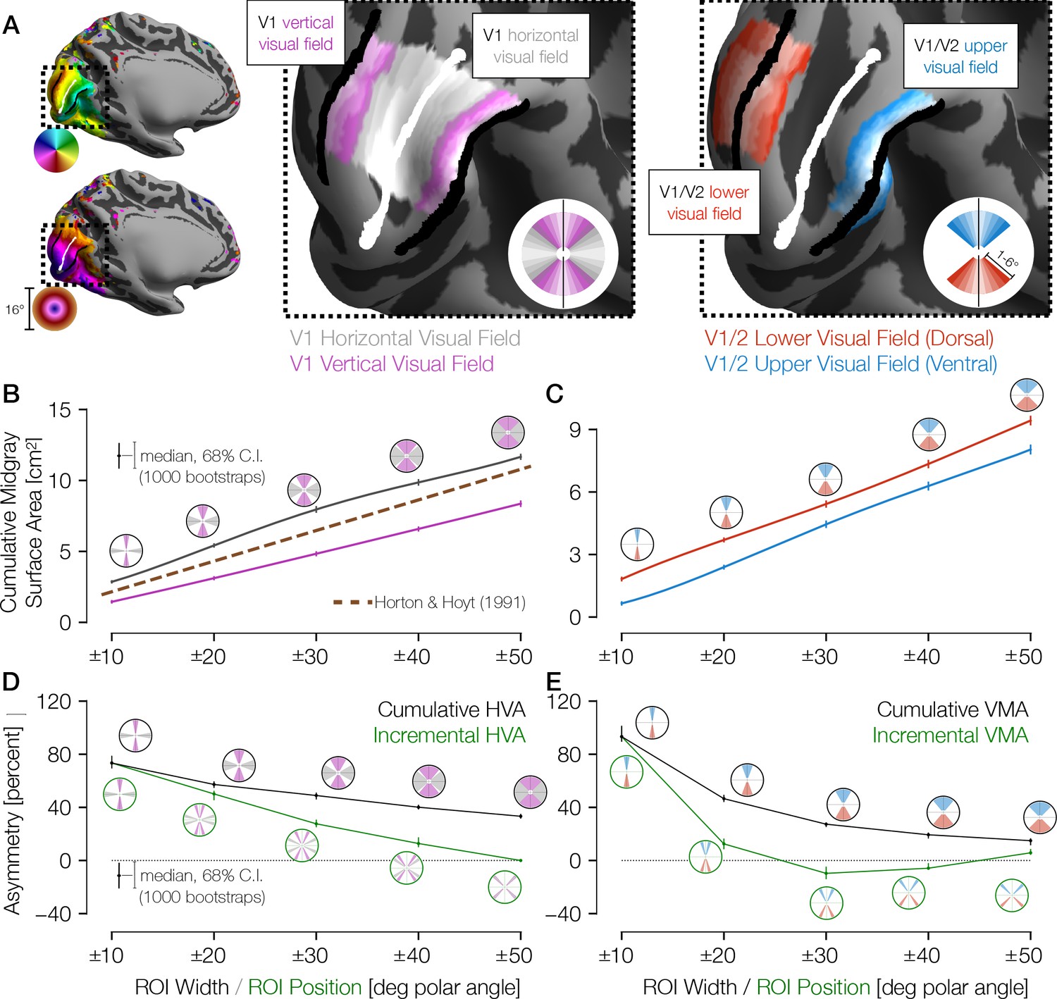
Cortical surface areas around the visual field.
(A) Polar angle (top left) and eccentricity (bottom left) maps for example HCP subject 177746. The V1/V2 boundaries and the V1 horizontal meridian obtained via Bayesian inference are shown as black and white lines, respectively. The middle panel of A shows ROIs drawn with gradually increasing polar angle widths centered around the horizontal meridian (gray) and the vertical meridian (V1/V2 boundary; magenta), limited to 1–6° of eccentricity in V1 only. The right panel shows ROIs around the upper vertical meridian (ventral V1/V2 boundary; blue) and the lower vertical meridian (dorsal V1/V2 boundary; red) that include both V1 and V2. In this hemisphere, the cortical surface area is greater near the horizontal than the vertical meridian and near the lower than the upper vertical meridian. (B) Mid-gray surface area for increasingly large ROIs centered on the vertical (magenta) or horizontal (gray) meridian. The error bars indicate the 68% confidence intervals (CIs) from bootstrapping. The circular icons show the visual field representations of the ROIs for the nearby data points. The x-values of data points were slightly offset in order to facilitate visualization. The brown dotted line shows the equivalent V1 ROI surface area as predicted by Horton and Hoyt, 1991. (C) Same as B, but for upper (blue) and lower (red) vertical meridians. (D, E) The surface areas are transformed to percent asymmetry, both for the cumulative ROIs (black) and incremental ROIs (green). Whereas cumulative ROIs represent a wedge of the visual field within a certain polar angle distance ± θ of a cardinal axis, incremental ROIs represent dual 10°-wide wedges in the visual field a certain polar angle distance ±θ from a cardinal axis. The percent asymmetry of x to y is defined as 100× (x−y)/mean(x, y). Positive values indicate greater area for horizontal than vertical (D) or for lower than upper regions (E). ROI, region of interest.
Figure 2—figure supplement 1
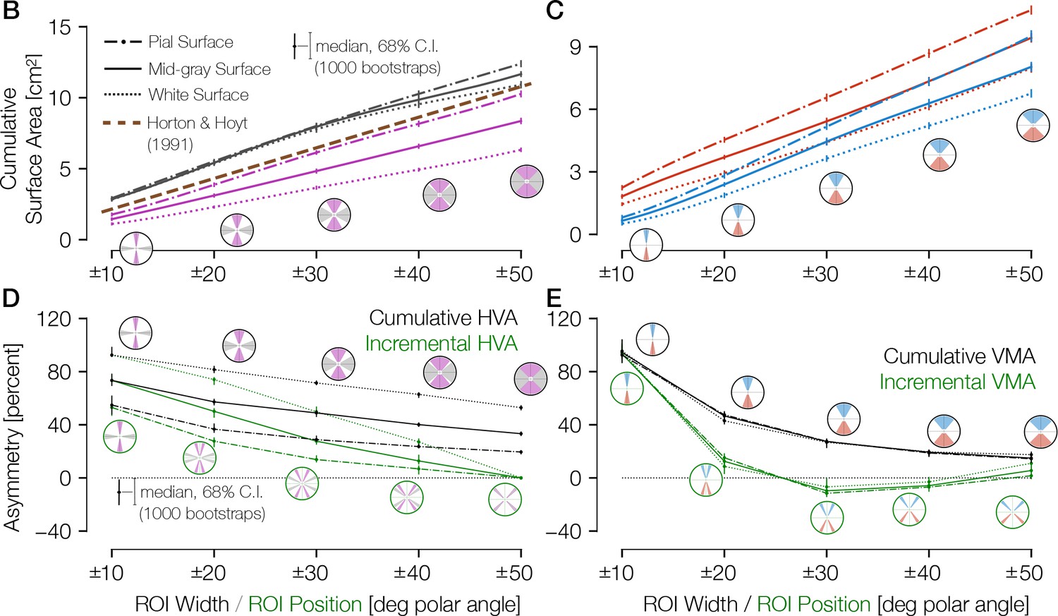
Pial, mid-gray, and white-matter surface areas around the visual field.
Surface area plots, as calculated in Figure 2, are shown with the addition of ROI surface areas calculated on both the pial and white-matter surfaces. No panel A is shown in order to match Figure 2. (B) Surface area for increasingly large ROIs centered on the vertical (magenta) or horizontal (gray) meridian. The error bars indicate the 68% CI from bootstrapping. The circular icons show the visual field representations of the ROIs for the nearby data points. The x-values of data points were slightly offset in order to facilitate visualization. The brown dotted line shows the equivalent V1 ROI surface area as predicted by Horton and Hoyt, 1991. (C) Same as B, but for upper (blue) and lower (red) vertical meridians. (D, E) The surface areas are transformed to percent asymmetry, both for the cumulative ROIs (black) and incremental ROIs (green). CI, confidence interval; ROI, region of interest.
Figure 3
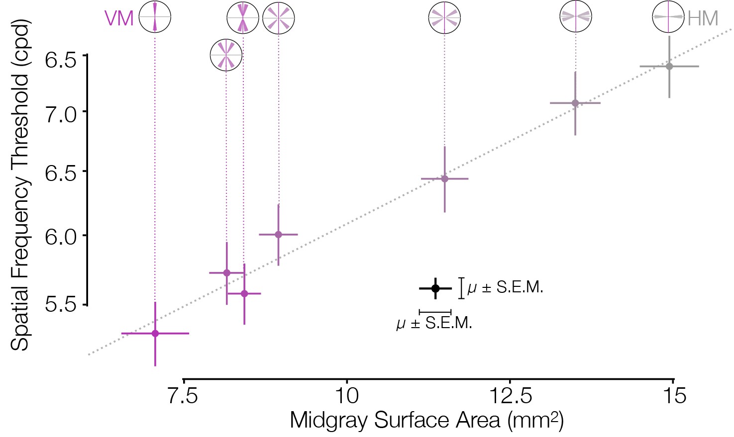
Asymmetries in behavior and cortical surface area are correlated in distinct subject groups.
V1 mid-gray surface area measured from the HCP dataset (Benson et al., 2018) is highly correlated with the spatial frequency thresholds measured by Barbot et al., 2021 in matched ROIs. Surface areas (x-axis) were computed for ROIs whose visual field positions were limited to 4–5° of eccentricity in order to match the psychophysical experiments. Areas were summed over regions indicated by the visual field insets (and divided by two for all ROIs except the VM and HM, since the latter two ROIs have half the visual field area of the other ROIs). The Pearson correlation is 0.99. HCP, Human Connectome Project; HM, horizontal meridian; ROI, region of interest; VM, vertical meridian.
Figure 4

Asymmetries in cortical surface area are correlated across twins.
Intraclass correlation (ICC) coefficient between twin pairs (monozygotic and dizygotic) and age- and gender-matched unrelated pairs. The correlations were computed for the HVA (left) and VMA (right) for wedge widths, as in Figure 2B and C. An unbiased estimate of the ICC was used (see Materials and methods). HVA, horizontal-vertical asymmetry; VMA, vertical meridian asymmetry.
Figure 5
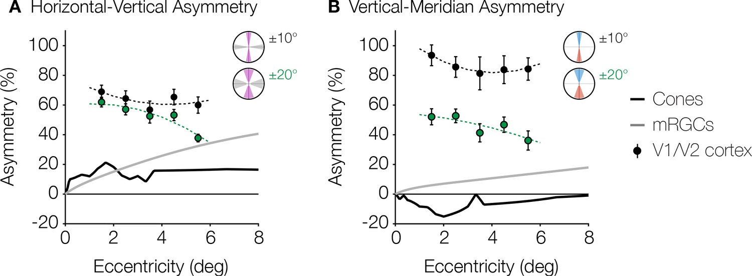
Asymmetries from retina and visual cortex.
(A) HVA and (B) VMA for cone density (black line) and mRGC density (gray line) when comparing the cardinal meridians, and V1/V2 cortical surface area within the ±10° ROIs (black markers) and ±20° ROIs (green markers) as a function of eccentricity. Cone density data are in counts/deg2 (Curcio et al., 1990). Midget RGC densities represent the receptive field counts/deg2 using the quantitative model by Watson, 2014. V1/V2 cortex data are calculated from the cortical surface area in mm2/deg2 within 1° non-overlapping eccentricity bands from 1° to 6° of the ±10° and ±20° ROIs. Markers and error bars represent the median and standard error across bootstraps, respectively. Data are fitted with a second-degree polynomial. HVA, horizontal-vertical asymmetry; RGC, retinal ganglion cell; ROI, region of interest; VMA, vertical meridian asymmetry.
Appendix 1—figure 1
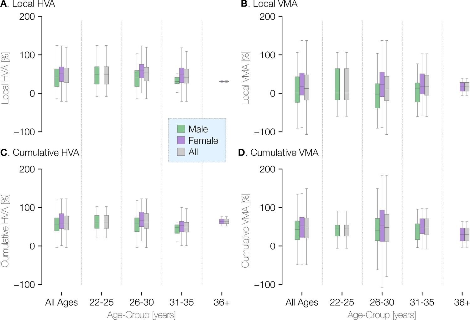
Visual field asymmetry in terms of age and gender at ±20° of polar angle.
Plots of the local (top row) and cumulative (bottom row) asymmetry across subjects in terms of age and gender. The percent horizontal-vertical asymmetry (HVA: horizontal ROI surface area minus vertical ROI surface area, divided by the mean surface area across horizontal and vertical ROIs) is shown in the left column, and the vertical meridian asymmetry (VMA: upper vertical ROI surface area minus lower vertical ROI surface area, divided by the mean surface area across upper and lower ROIs) is shown in the right column. Box-plots show the median (central horizontal line), quartiles (shaded box), and ±95% percentiles (lines).
Appendix 1—figure 2

V1 size and volume differences in terms of sex.
ROI is limited to V1 between 1° and 6° of eccentricity. Violin plots terminate at the exact extrema of the dataset. Surface area was calculated on the mid-gray surface. Volume calculations include the entire gray-matter layer. Whole-hemisphere calculations for surface area and volume exclude the region corresponding to the corpus callosum.
Appendix 1—figure 3
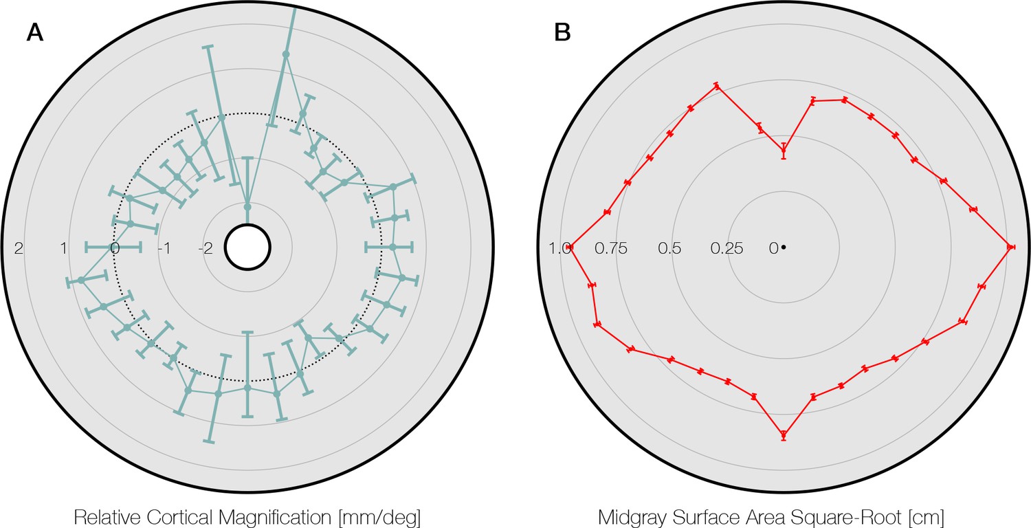
Comparison to Silva et al., 2018.
(A) Data from Silva et al., 2018; Figure 4, replotted around the visual field. The gray area of the panel indicates the axis limits of the original plot. Plot points and confidence intervals represent the linear cortical magnification of each polar angle bin after regressing out the effect of eccentricity on cortical magnification. (B) The square root of the mid-gray surface area of the 163 subjects analyzed in this paper, plotted for polar angle bins matched to those in panel A. Bins were limited to between 1° and 6° of eccentricity. The square-root of the surface area is used because it should scale linearly with the linear cortical magnification values plotted by Silva et al., 2018 and replotted in panel A. Notably, the LVM has a substantially higher surface area in panel B than the points around it. This is likely due to the prevalence of ipsilateral pRFs near the LVM (Gibaldi et al., 2021). Our method does not explicitly account for ipsilateral representation, and thus parts of cortex with ipsilateral pRFs will tend to be counted as part of the vertical meridian when the polar angle bins are sufficiently small (see also Methods). Thus the data point at the LVM should be read and interpreted with caution. pRF, population receptive field. LVM, lower vertical meridian.
Additional files
Download links
A two-part list of links to download the article, or parts of the article, in various formats.
Downloads (link to download the article as PDF)
Open citations (links to open the citations from this article in various online reference manager services)
Cite this article (links to download the citations from this article in formats compatible with various reference manager tools)
Cortical magnification in human visual cortex parallels task performance around the visual field
eLife 10:e67685.
https://doi.org/10.7554/eLife.67685


