Topological network analysis of patient similarity for precision management of acute blood pressure in spinal cord injury
- Weill Institute for Neurosciences; Brain and Spinal Injury Center (BASIC), Department of Neurological Surgery, University of California, San Francisco; Zuckerberg San Francisco General Hospital and Trauma Center, United States
- Division of Physical Medicine and Rehabilitation, Department of Orthopaedics and Rehabilitation, University of New Mexico School of Medicine, United States
- San Francisco Veterans Affairs Healthcare System, United States
- Computational Research Division, Lawrence Berkeley National Laboratory, United States
- Lawrence Berkeley National Laboratory, United States
- Rehabilitation Research Center, Santa Clara Valley Medical Center, United States
- Department of Psychiatry and Behavioral Science, and University of Minnesota, United States
- Institute for Health Informatics, University of Minnesota, United States
- Department of Radiology and Biomedical Imaging, University of California, San Francisco, United States
- Department of Emergency Medicine, University of California, San Francisco; Zuckerberg San Francisco General Hospital and Trauma Center, United States
- Department of Physical Medicine and Rehabilitation, Santa Clara Valley Medical Center, United States
- Department of Neurosurgery, Stanford University, United States
- Department of Anesthesia and Perioperative Care, University of California, San Francisco; Zuckerberg San Francisco General Hospital and Trauma Center, United States
Figures
Figure 1
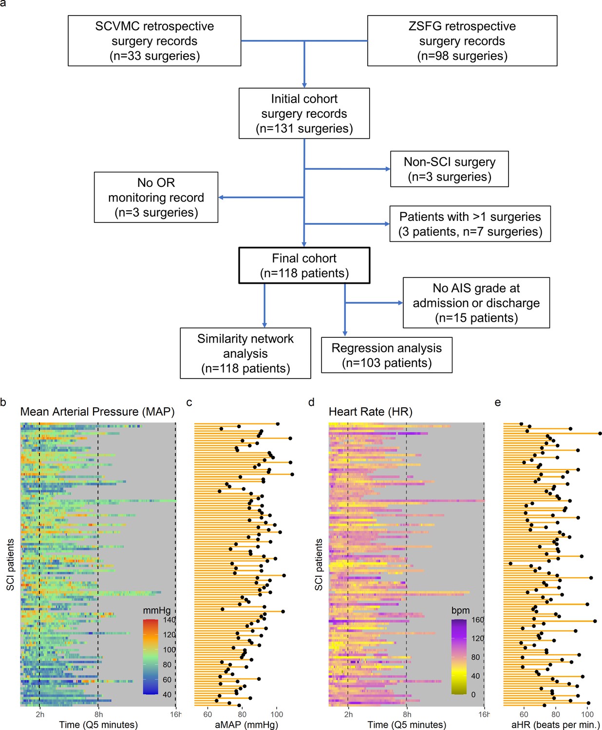
High-frequency monitoring operating room (OR) data.
Flowchart of retrospective study and cohort selection criteria (a). A final cohort of 118 patients were identified and values of mean arterial pressure (MAP) (b) and heart rate (HR), (c) by time (bins of 5 min; Q5) retrospectively extracted from patients’ records. Colormaps represent the MAP (mmHg; green marks normotensive MAP, while blue and red marks hypotension and hypertension, respectively) and HR (beats per min, bpm; dark yellow lowest to purple highest) at each Q5 time, depicting the temporal fluctuation of each measure for each patient (row). The average MAP (aMAP, right plot in b) and average heart rate (aHR, right plot in c) were computed.
Figure 2 with 2 supplements
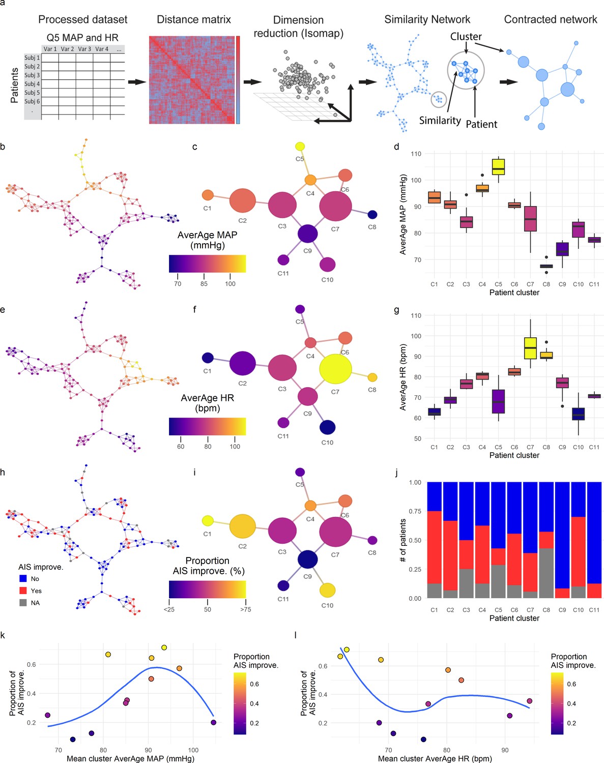
Topological network analysis of intra-operative monitoring.
Intra-operative mean arterial pressure (MAP) and heart rate (HR) sampled every 5 min (Q5) were curated, processed, and formatted in a unique data matrix (a) (Figure 2—figure supplement 1). The similarity matrix between patients was computed and a four-dimensional subspace extracted using Isomap (Figure 2—figure supplement 1). A network was constructed where nodes represent patients and edges the connection of pairs of patients under a specified threshold of similarity (see Methods). The network was clustered and collapsed (Figure 2—figure supplement 1) by using the walktrap algorithm conveying in 11 clusters. These networks captured both the average MAP (aMAP) (b–d) and the average HR (aHR) (e–g) in a gradient fashion. Similarly, at least one AIS grade gain at discharge (‘yes’, ‘no’) was mapped over the network (h–j, gray: 15 AIS grades could not be extracted). Clusters of higher proportion of patients with recovery had an aMAP in a middle range, while clusters with higher proportion of patients without recovery presented extreme aMAPs (k). The mean cluster aHR showed a less apparent relationship with the proportion of AIS improvers (l).
Figure 2—figure supplement 1
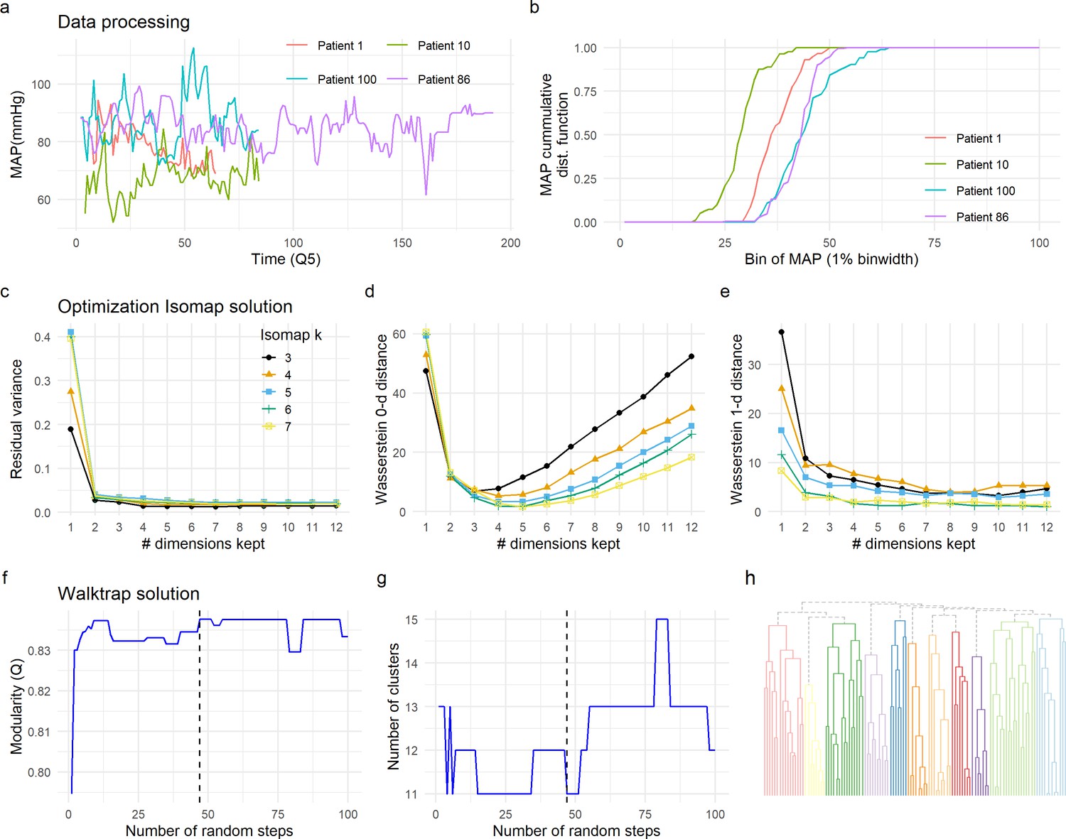
Data preprocessing, dimensionality reduction, and clustering optimization.
The time-series signal between patients is not aligned (changes at specific time point might not reflect the same for each patient) and of different length due to the different duration of surgery (a). To be able to compute a distance metric between patients, we pre-processed the time-series data by calculating the cumulative distribution function (CDF) of each signal and each patient (b, see Methods). CDF was then used to compute the similarity between patients (Figure 2b, see Methods), input of Isomap for dimension reduction (Figure 2c). Two criteria were used to select the optimal solution for the Isomap. We first sought the solution that preserved major information in terms of the similarity between patients (distance metric) by minimizing the residual variance (c). We considered the minimal k being the one that produced a continuous (non-fragmented) k-NNG (k = 3). Residual variance was compared for different solutions of Isomap (3≤ k ≤ 7), without major differences between solutions, except for the first dimension (see Methods). This first analysis also suggested the real dimensionality of the data to be around three to four dimensions by looking at the ‘elbow’ in which no more substantial information would be added. We then selected the solution that minimized the loss of topological information by persistent homology. Wasserstein zero-dimensional (WD0, d) and one-dimensional (WD1, e) distances were computed. A final solution of k = 6 and 4 Isomap dimensions was chosen for being the one minimizing WD0 and WD1. Walktrap algorithm was chosen for network clustering. To determine the optimal number of random steps, an increasing number of steps were set and modularity (Q) computed (f). The first solution that maximized Q (Q = 0.837) was selected (dashed line in f and g). The optimal solution determined 11 clusters (h).
Figure 2—figure supplement 2
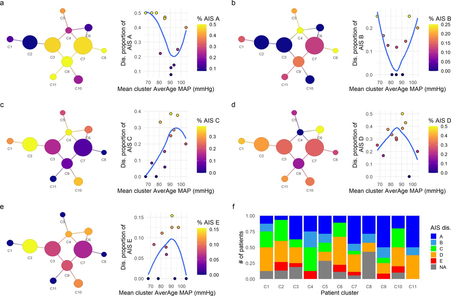
Exploratory network analysis of AIS (American Spinal Injury Association [ASIA] Impairment Scale) at discharge.
The proportion of AIS grades at discharge for each cluster was mapped into the network and its association with the mean average mean arterial pressure (aMAP) per cluster explored. Clusters with lower proportion of AIS A (a) and AIS B (b) were associated with central mean aMAP values (~90 mmHg in AIS A and 80–90 mmHg in AIS B) with higher proportion of those AIS grades at the extremes of mean aMAP. Contrary, AIS C (c), AIS D (d), and AIS E (e) at discharge showed the inverse relationship, clusters with higher proportion of AIS C, D, and E were associated with middle ranges of mean aMAP, while cluster with lower proportion of those grades trended to have extreme values of mean aMAP. This suggests that the population of patients with extreme values of aMAP had higher probability to be discharged with AIS A and B grades, while patients with central values of aMAP had higher probability of discharge with AIS C, D, and E. Moreover, the clusters with higher proportion of AIS improvers (C1, C2, C4, and C10, Figure 2) also showed higher proportions of AIS C, D, and E at discharge (f) than the clusters with lower proportion of improvers (C5, C8, C9, C11, Figure 2). These results further support the hypothesis that both hypotensive and hypertensive MAP during surgery is related with lower probability of recovery of at least one AIS grade at discharge. Trend lines (blue) were plotted to aid visual exploratory analysis.
Figure 3
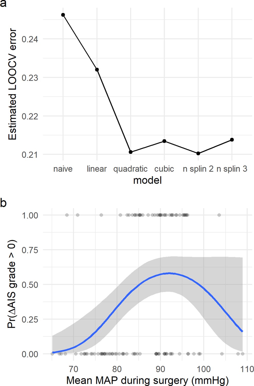
Non-linear relationship of average mean arterial pressure (aMAP) with the probability of improving at least one AIS grade.
Logistic regression models were fitted to study the potential non-linearity of the aMAP predictor as suggested by the exploratory analysis. Six different models were studied: naïve, linear, quadratic, cubic, spline of degree 2, and spline of degree 3. The estimated leave-one-out cross-validation (LOOCV) error for each model showed that both the quadratic and the spline of degree 2 have the minimal cross-validation error (a). This suggests that the linear model did not capture all the potential explainable variance of the response variable by aMAP, while the cubic and spline of degree 3 were probably overfitting the model (Table 2). (b) shows the logit function (blue line) and standard error (gray ribbon) of the quadratic model over the fitted values (points).
Figure 4 with 3 supplements
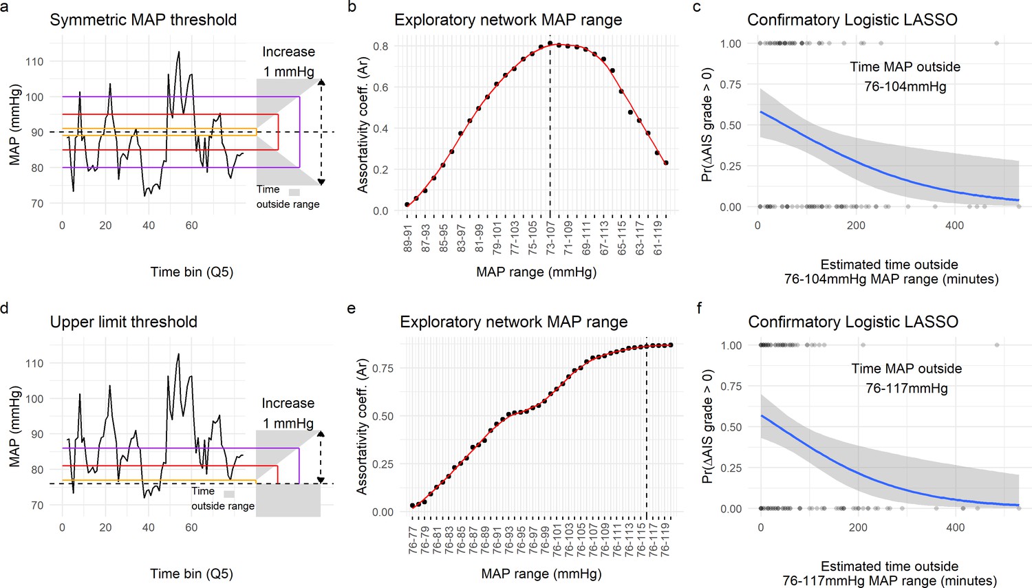
Range of mean arterial pressure (MAP).
To find the optimal MAP range, a moving MAP range was computed and the time of MAP outside range calculated (a and d, example of the same patient for symmetric and asymmetric map range, respectively). Calculating the assortativity coefficient (Ar) of the network for each range revealed that the distribution of patients in the network was most highly associated with the range 73–107 mmHg for the symmetric range (b, Figure 4—figure supplement 1), and 76–116 mmHg for the asymmetric range study of upper limit threshold (e, Figure 4—figure supplement 1). A logistic LASSO (least absolute shrinkage and selection operator) regression (Figure 4—figure supplement 2a, Figure 4—figure supplement 3) was used as a confirmatory analysis and to obtain the MAP range that most highly predicts AIS grade recovery. For the symmetric range, the time of MAP outside the 76–104 mmHg (c, Table 10) was found to be the ‘last-standing’ predictor during LASSO regularization (Figure 4—figure supplement 2a), suggesting that greater duration outside this range is associated with lower probability of neurological recovery. In the case of the asymmetric range (Figure 4—figure supplement 3), the last non-zero coefficient was for the range 76–117 mmHg (f, Table 11).
Figure 4—figure supplement 1
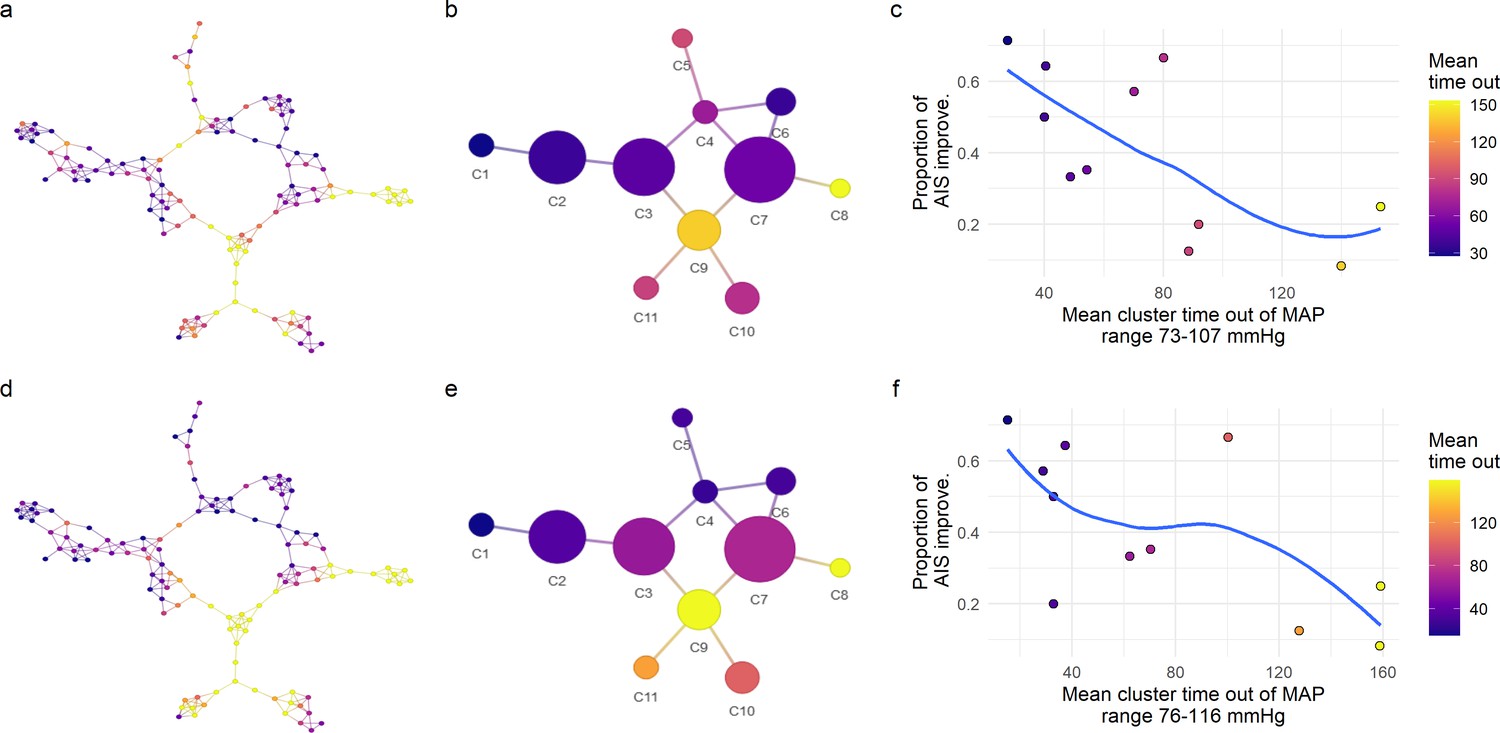
Exploratory network analysis of mean arterial pressure (MAP) out of range.
We further explored the relationship of the distribution of patients in the network and the amount of time their MAP was out of a specific range (Figure 4). For each MAP range, the assortativity coefficient (Ar) was calculated (Figure 4). The major Ar was achieved when considering the time of MAP out of the range 73–107 mmHg for the symmetric range (a–c), and the range 76–116 mmHg for the asymmetric one (d–f). Mapping those values of time into the similarity network (a), we observe patients with the longest times or patients with the shortest times were localized together, indicating that the network was capturing the clustering structure associated with time of MAP out of the specific range. The mean time out of that range per cluster presented an inverse relationship with its proportion of AIS improvers (c and f) where clusters of patients with longer times of MAP out of range has lower proportion of AIS improvers. This reinforced the hypothesis that low probability of improvement at least one AIS at discharge is related with the amount of time MAP is out of a lower and upper boundary. Consequently, we performed confirmatory analysis of this hypothesis using a logistic LASSO (least absolute shrinkage and selection operator) regression (Figure 4 and Figure 4—figure supplement 2a, Figure 4—figure supplement 3). Trend lines (blue) are plotted to aid visual exploratory analysis.
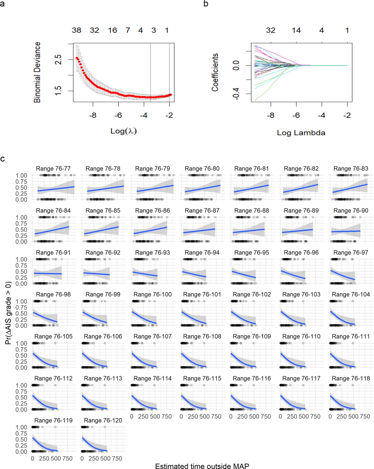
Figure 4—figure supplement 2
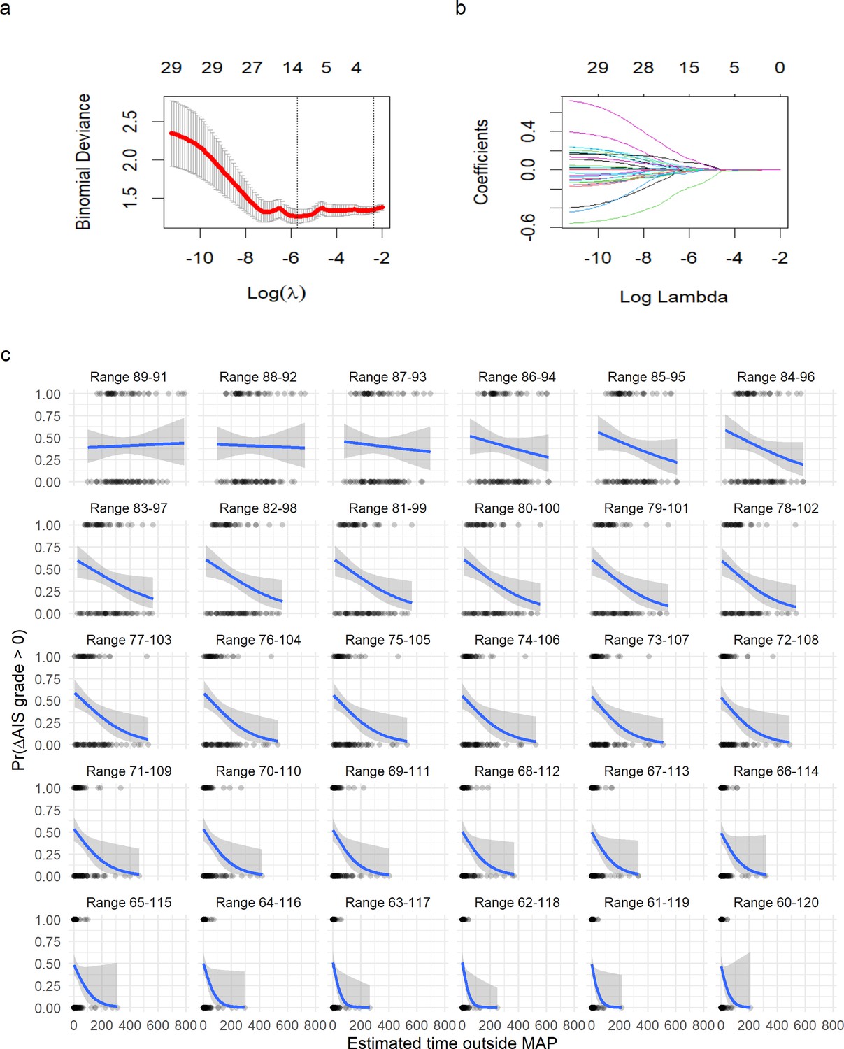
Logistic least absolute shrinkage and selection operator (LASSO) regression with leave-one-out cross-validation (LOOCV) of symmetric range.
(a) The deviance of the binomial model used as cross-validation error (mean and standard deviation) in the LOOCV (see Methods) against the values of l (in log form). The two vertical doted lines express the model that produces the minimal error (left line) and the first model to reach one standard deviation from the minimal error (see Methods). (b) The coefficients (each colored line) for a given value of l (in log form). The values on top in (a) and (b) express the number of non-zero coefficients for a given l. A value of l = 0.121 shrinks the model to one single predictor (time of MAP out of range 76–104). A logistic regression for time of MAP out of range 76–104 was then fitted (Figure 4). (c) Plots of fitting a logistic regression for each range of MAP. It can be appreciated how as the range of MAP gets wider, the relationship of time out of range and probability of AIS improvement gets stronger until a point where the range is too wide to discriminate between AIS improvers and non-improvers.
Figure 4—figure supplement 3
Logistic least absolute shrinkage and selection operator (LASSO) regression with leave-one-out cross-validation (LOOCV) of asymmetric range.
Figure 5
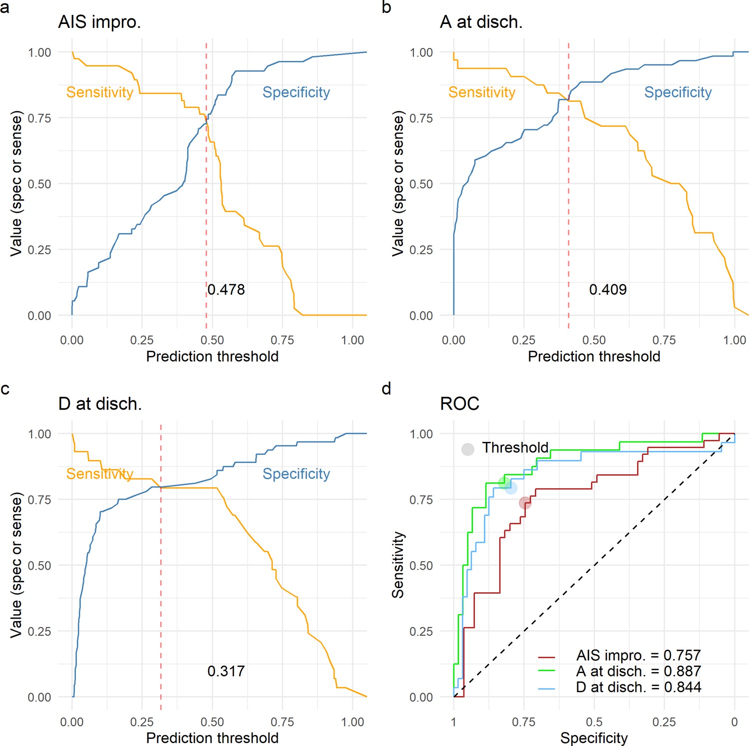
Leave-one-out cross-validation (LOOCV) performance of prediction models.
We built three prediction models, one to predict American Spinal Injury Association (ASIA) Impairment Scale (AIS) improvement of at least one grade at discharge (AIS impro., a), one to predict AIS A at discharge (A at disch., b) and one to predict AIS D at discharge (D at disch., c). The sensitivity and specificity for each model was computed out of the prediction probability of LOOCV, where each leave-one-out patient is predicted with the model that was trained without that patient. For each model, the classification threshold was set at the probability that balances sensitivity and specificity (dashed red line). The receiving operation curve (ROC) and area under the curve (AUC) for the three models are presented in d.
Tables
Table 1
Cohort demographics split by AIS (American Spinal Injury Association [ASIA] Impairment Scale) improvement.
| AIS improve. N/A(n = 15) | AIS improve. NO(n = 61) | AIS improve. YES(n = 42) | Univariate p-value | |
|---|---|---|---|---|
| Age (years) | 0.12 | |||
| Mean (SD) | 46.0 (17.6) | 45.3 (19.1) | 51.4 (19.7) | |
| Median [min, max] | 45.5 [19.0, 87.0] | 47.0 [18.0, 82.0] | 55.0 [18.0, 86.0] | |
| Missing | 1 (6.7%) | 2 (3.3%) | 1 (2.4%) | |
| AIS admission | 0.013 | |||
| A | 1 (6.7%) | 33 (54.1%) | 18 (42.9%) | |
| B | 0 (0%) | 5 (8.2%) | 8 (19.0%) | |
| C | 0 (0%) | 5 (8.2%) | 11 (26.2%) | |
| D | 0 (0%) | 14 (23.0%) | 5 (11.9%) | |
| E | 0 (0%) | 4 (6.6%) | 0 (0%) | |
| Missing | 14 (93.3%) | 0 (0%) | 0 (0%) | |
| AIS discharge | <0.0001 | |||
| A | 0 (0%) | 35 (57.4%) | 0 (0%) | |
| B | 0 (0%) | 5 (8.2%) | 5 (11.9%) | |
| C | 1 (6.7%) | 4 (6.6%) | 15 (35.7%) | |
| D | 0 (0%) | 14 (23.0%) | 17 (40.5%) | |
| E | 1 (6.7%) | 2 (3.3%) | 5 (11.9%) | |
| Missing | 13 (86.7%) | 1 (1.6%) | 0 (0%) | |
| Surgery duration (min) | 0.66 | |||
| Mean (SD) | 433 (167) | 392 (146) | 407 (181) | |
| Median [min, max] | 432 [121, 725] | 389 [120, 728] | 343 [151, 950] | |
| Missing | 1 (6.7%) | 2 (3.3%) | 1 (2.4%) | |
| Surgery to discharge (days) | 0.33 | |||
| Mean (SD) | 9.50 (2.12) | 18.8 (20.6) | 23.4 (23.8) | |
| Median [min, max] | 9.50 [8.00, 11.0] | 11.0 [1.00, 128] | 14.5 [4.00, 120] | |
| Missing | 13 (86.7%) | 4 (6.6%) | 2 (4.8%) | |
| Dichotomized neurological level of injury at admission | 0.054 | |||
| Cervical | 2.00 (13.3%) | 36 (59%) | 33 (78.6%) | |
| Non-cervical | 13.00 (86.7%) | 25 (41%) | 9 (21.4%) |
Table 2
Logistic regression likelihood ratio test and leave-one-out cross-validation (LOOCV) error (n = 103 patients).
| Model | AIC | Residual df | Residualdeviance | Deviance | p-Value | LOOCV error |
|---|---|---|---|---|---|---|
| Null model | 141.26 | 102 | 139.26 | 0.246 | ||
| Linear model | 134.8 | 101 | 130.80 | 8.46(vs. null model) | 0.0036**(vs. null model) | 0.231 |
| Quadratic model | 128.48 | 100 | 122.48 | 8.32(vs. linear model) | 0.0039**(vs. linear model) | 0.210 |
| Cubic model | 126.97 | 99 | 118.97 | 3.50(vs. quadratic model) | 0.061(vs. quadratic model) | 0.213 |
| Natural Spline model (df = 2) | 128.29 | 100 | 122.29 | 8.50(vs. linear model) | 0.0035**(vs. linear model) | 0.210 |
| Natural Spline model (df = 3) | 127.13 | 99 | 119.13 | 3.34(vs. quadratic model) | 0.067(vs. quadratic model) | 0.213 |
-
** p < 0.01.
Table 3
Evaluation of logistic regression (Wald test) and leave-one-out cross-validation (LOOCV) error.
| Model: where average MAP (n = 103 patients) | ||||
|---|---|---|---|---|
| LOOCV: average observed accuracy = 0.66; average kappa statistic = 0.334 | ||||
| Predictor | Coef. estimate (logit) | Std. error | z-Value | p-Value |
| Intercept | = –0.55 | 0.242 | –2.293 | 0.02183* |
| Average MAP () | = 8.62 | 2.944 | 2.931 | 0.00338** |
| Average MAP () | = –7.601 | 3.039 | –2.501 | 0.0123* |
-
*p < 0.05; **p < 0.01.
Table 4
Evaluation of logistic regression with covariates (Wald test) and leave-one-out cross-validation (LOOCV).
| Model: , where average MAP; : average HR; length of surgery (min); days to AIS discharge (days); age; AIS admission D (‘yes’,’no’); AIS admission C (‘yes’,’no’); AIS admission B (‘yes’,’no’); AIS admission A (‘yes’,’no’); (AIS admission E was set as the reference level for AIS admission variable and is part of the intercept) (final n = 93) | |||||||||
|---|---|---|---|---|---|---|---|---|---|
| LOOCV: average observed accuracy = 0.688; average kappa statistic = 0.362 | |||||||||
| Predictor | Coef. estimate (logit) | Std. error | z-Value | p-Value | |||||
| Intercept | = –1.530 | 121.8 | –0.013 | 0.99 | |||||
| Average MAP () | = 7.398 | 3.112 | 2.377 | 0.017* | |||||
| Average MAP () | = –8.053 | 3.530 | –2.281 | 0.022* | |||||
| Average HR () | = –2.087 | 0.0245 | –0.851 | 0.394 | |||||
| Length of surgery () | = 0.0011 | 0.0015 | 0.728 | 0.466 | |||||
| Days to AIS discharge () | = 0.0037 | 0.0109 | 0.344 | 0.730 | |||||
| Age () | = 0.0082 | 0.013 | 0.634 | 0.526 | |||||
| AIS admission D () | = 1.454 | 1.218 | 0.012 | 0.990 | |||||
| AIS admission C () | = 1.645 | 1.218 | 0.014 | 0.989 | |||||
| AIS admission B () | = 1.585 | 1.218 | 0.013 | 0.989 | |||||
| AIS admission A () | = 1.527 | 1.218 | 0.013 | 0.990 | |||||
| Correlation matrix (Spearman) | |||||||||
| Average MAP | AverageHR | Length of surgery | Days to AIS discharge | Age | AIS admission | ||||
| Average MAP | 1 | ||||||||
| Average HR | –0.126 | 1 | |||||||
| Length of surgery | –0.152 | 0.101 | 1 | ||||||
| Days to AIS discharge | 0.088 | –0.059 | 0.165 | 1 | |||||
| Age | 0.006 | –0.245 | 0.011 | 0.022 | 1 | ||||
| AIS admission | 0.024 | 0.003 | –0.01 | 0.258 | –0.13 | 1 | |||
-
*p < 0.05.
Table 5
Evaluation of logistic regression covariates only (Wald test) and leave-one-out cross-validation (LOOCV).
| Model: , where : average HR; length of surgery (min); days to AIS discharge (days); age; AIS admission D (‘yes’,’no’); AIS admission C (‘yes’,’no’); AIS admission B (‘yes’,’no’); AIS admission A (‘yes’,’no’); (AIS admission E was set as the reference level for AIS admission variable and is part of the intercept) (final n = 93) | ||||
|---|---|---|---|---|
| LOOCV: average observed accuracy = 0.612; average kappa statistic = 0.17 | ||||
| Predictor | Coef. estimate (logit) | Std. error | z-Value | p-Value |
| Intercept | = –1.585 | 138.2 | –0.011 | 0.991 |
| Average HR () | = –0.0209 | 0.029 | –0.911 | 0.362 |
| Length of surgery () | = 0.0016 | 0.00141 | 1.151 | 0.250 |
| Days to AIS discharge () | = 0.0105 | 0.0106 | 0.993 | 0.320 |
| Age () | = 0.0052 | 0.012 | 0.424 | 0.672 |
| AIS admission D () | = 1.511 | 1.382 | 0.011 | 0.991 |
| AIS admission C () | = 1.715 | 1.382 | 0.012 | 0.991 |
| AIS admission B () | = 1.643 | 1.382 | 0.012 | 0.990 |
| AIS admission A () | = 1.574 | 1.382 | 0.011 | 0.991 |
Table 6
Evaluation of logistic regression in American Spinal Injury Association (ASIA) Impairment Scale (AIS) A at admission cohort (Wald test) and leave-one-out cross-validation (LOOCV).
| Model: , where average MAP; : average HR; length of surgery (min); days to AIS discharge (days); age (final n = 51) | ||||
|---|---|---|---|---|
| LOOCV: average observed accuracy = 0.63; average kappa statistic = 0.197 | ||||
| Predictor | Coef. estimate (logit) | Std. error | z-Value | p-Value |
| Intercept | = –0.931 | 3.433 | –0.271 | 0.786 |
| Average MAP () | = 10.79 | 5.014 | 2.153 | 0.031* |
| Average MAP () | = –6.73 | 4.591 | –1.468 | 0.142 |
| Average HR () | = –0.016 | 0.035 | –0.468 | 0.639 |
| Length of surgery () | = 0.0039 | 0.0026 | 1.504 | 0.132 |
| Days to AIS discharge () | = 0.0067 | 0.014 | 0.477 | 0.633 |
| Age () | = –0.012 | 0.020 | –0.599 | 0.549 |
-
*p < 0.05.
Table 7
Neurological level of injury cases.
| Cervical (n = 71) | Non-cervical (n = 32) | |||||||||||||||||||
|---|---|---|---|---|---|---|---|---|---|---|---|---|---|---|---|---|---|---|---|---|
| NLI | C2 | C3 | C4 | C5 | C6 | C7 | C8 | T2 | T3 | T4 | T5 | T6 | T7 | T8 | T9 | T10 | T11 | T12 | S1 | S5 |
| Cases | 3 | 3 | 24 | 28 | 4 | 8 | 1 | 1 | 3 | 3 | 1 | 2 | 1 | 3 | 1 | 3 | 2 | 4 | 6 | 2 |
Table 8
Evaluation of logistic regression in Cervical cohort (Wald test) and leave-one-out cross-validation (LOOCV).
| Model: , where average MAP; : average HR; length of surgery (min); days to AIS discharge (days); age; AIS admission D (‘yes’,’no’); AIS admission C (‘yes’,’no’); AIS admission B (‘yes’,’no’); (AIS admission A was set as the reference level for AIS admission variable and is part of the intercept, no AIS admission E was present in this cohort) (final n = 93) | ||||
|---|---|---|---|---|
| LOOCV: average observed accuracy = 0.688; average kappa statistic = 0.362 | ||||
| Predictor | Coef. estimate (logit) | Std. error | z-Value | p-Value |
| Intercept | = 2.747 | 3.018 | 0.91 | 0.363 |
| Average MAP () | = 7.594 | 3.056 | 2.485 | 0.013* |
| Average MAP () | = –7.528 | 3.358 | –2.242 | 0.025* |
| Average HR () | = –0.055 | 0.034 | –1.608 | 0.108 |
| Length of surgery () | = 0.0014 | 0.0019 | 0.720 | 0.472 |
| Days to AIS discharge () | = 0.0022 | 0.012 | 0.182 | 0.855 |
| Age () | = 0.0079 | 0.016 | 0.482 | 0.630 |
| AIS admission D () | = –0.747 | 0.87 | –0.840 | 0.730 |
| AIS admission C () | = 0.745 | 0.80 | 0.925 | 0.355 |
| AIS admission B () | = 0.301 | 0.88 | 0.346 | 0.401 |
-
*p < 0.05.
Table 9
Evaluation of logistic regression in non-cervical cohort only (Wald test) and leave-one-out cross-validation (LOOCV).
| Model: , where average MAP; : average HR; length of surgery (min); days to AIS discharge (days); age; AIS admission D (‘yes’,’no’); AIS admission C (‘yes’,’no’); AIS admission B (‘yes’,’no’); AIS admission A (‘yes’,’no’); (AIS admission E was set as the reference level for AIS admission variable and is part of the intercept) (final n = 93) | ||||
|---|---|---|---|---|
| LOOCV: average observed accuracy = 0.688; average kappa statistic = 0.362 | ||||
| Predictor | Coef. estimate (logit) | Std. error | z-Value | p-Value |
| Intercept | = –1.883 | 352.4 | –0.005 | 0.996 |
| Average MAP () | = –0.206 | 4.713 | –0.044 | 0.965 |
| Average MAP () | = –8.064 | 7.643 | –1.055 | 0.291 |
| Average HR () | = –0.0002 | 0.0649 | 0.004 | 0.997 |
| Length of surgery () | = 0.0018 | 0.0054 | 0.336 | 0.737 |
| Days to AIS discharge () | = 0.076 | 0.0613 | 1.240 | 0.215 |
| Age () | = –0.0047 | 0.051 | –0.921 | 0.357 |
| AIS admission D () | = 1.727 | 3.524 | 0.005 | 0.996 |
| AIS admission C () | = 3.557 | 5.782 | 0.005 | 0.996 |
| AIS admission B () | = 1.738 | 3.524 | 0.005 | 0.995 |
| AIS admission A () | = 1.686 | 3.524 | 0.005 | 0.996 |
Table 10
Least absolute shrinkage and selection operator (LASSO) solution and logistic regression of most predictive symmetric range with leave-one-out cross-validation (LOOCV).
| Model: , where time of MAP outside range 76–104 mmHg (n = 103 patients) | ||||
|---|---|---|---|---|
| LOOCV: average observed accuracy = 0.61; average kappa statistic = 0.158 | ||||
| Predictor | Coef. estimate (logit) | Std. error | z-Value | p-Value |
| Intercept | = 0.368 | 0.333 | 1.103 | 0.269 |
| Time MAP out 76–104 () | = –0.006 | 0.0026 | –2.566 | 0.0103* |
-
*p < 0.05.
Table 11
Least absolute shrinkage and selection operator (LASSO) solution and logistic regression of most predictive asymmetric range with leave-one-out cross-validation (LOOCV).
| Model: , where time of MAP outside range 76–117 mmHg (n = 103 patients) | ||||
|---|---|---|---|---|
| LOOCV: average observed accuracy = 0.5728; average kappa statistic = 0.102 | ||||
| Predictor | Coef. estimate (logit) | Std. error | z-Value | p-Value |
| Intercept | = 0.2881 | 0.287 | 1.002 | 0.316 |
| Time MAP out 76–117 () | = –0.00788 | 0.0027 | –2.828 | 0.00468** |
-
**p < 0.01.
Table 12
Best prediction models of outcome.
| Model predicting AIS improvement: Model predicting AIS A: Model predicting AIS D: where average MAP; : AIS admission A (‘yes’, ‘no’); : AIS admission B (‘yes’, ‘no’); : AIS admission C (‘yes’, ‘no’); : AIS admission D (‘yes’, ‘no’); : NLI non-cervical; : Time MAP out 76–117; : Length of surgery; : Age; (AIS admission E and NLI cervical were set as the reference levels for the corresponding variable and are part of the intercept). All metrics are on LOOCV prediction (n = 93) | |||
|---|---|---|---|
| Model AIS improv. | Model AIS A | Model AIS D | |
| Predictor | Coef. estimate (logit) | Coef. estimate (logit) | Coef. estimate (logit) |
| Intercept | = –16.24 | = 20.466 | = 1.558 |
| Average MAP () | = 7.374 | = 27.031 | |
| Average MAP (Cohn et al., 2010) () | = –8.215 | = –17.138 | |
| AIS admission A () | = 15.54 | = –22.814 | = 2.324 |
| AIS admission B () | = 16.1818 | = –20.38 | = 0.41 |
| AIS admission C () | = 16.752 | = –19.01 | = –2.591 |
| AIS admission D () | = 14.828 | = 0.217 | = –2.624 |
| NLI non-Cervical () | = –1.228 | ||
| Time MAP out 76–117 () | = 0.017 | ||
| Length of Surgery () | = –0.0044 | ||
| Age () | = 0.03 | ||
| Model performance metric | Metric value | Metric value | Metric value |
| Accuracy (95% CI) | 0.73 (0.629, 0.818) | 0.82 (0.735, 0.898) | 0.806 (0.71, 0.881) |
| AUC | 0.743 | 0.88 | 0.87 |
| Kappa | 0.45 | 0.629 | 0.573 |
| Sensitivity | 0.71 | 0.812 | 0.793 |
| Specificity | 0.74 | 0.836 | 0.812 |
| Positive predicted value | 0.658 | 0.72 | 0.657 |
| Negative predicted value | 0.788 | 0.89 | 0.896 |
Additional files
-
Supplementary file 1
Code.output.html: output html file results of running the source code.
- https://cdn.elifesciences.org/articles/68015/elife-68015-supp1-v4.zip
-
Source code 1
Source.code.Rmd: Rmarkdown file containing the source code that reproduced the paper.
- https://cdn.elifesciences.org/articles/68015/elife-68015-supp2-v4.zip
-
Transparent reporting form
- https://cdn.elifesciences.org/articles/68015/elife-68015-transrepform1-v4.docx
Download links
A two-part list of links to download the article, or parts of the article, in various formats.
Downloads (link to download the article as PDF)
Open citations (links to open the citations from this article in various online reference manager services)
Cite this article (links to download the citations from this article in formats compatible with various reference manager tools)
Topological network analysis of patient similarity for precision management of acute blood pressure in spinal cord injury
eLife 10:e68015.
https://doi.org/10.7554/eLife.68015


