Multilayer brain networks can identify the epileptogenic zone and seizure dynamics
- Signal and Image Processing Institute, University of Southern California, United States
- Epilepsy Center, Cleveland Clinic Neurological Institute, United States
Figures
Figure 1
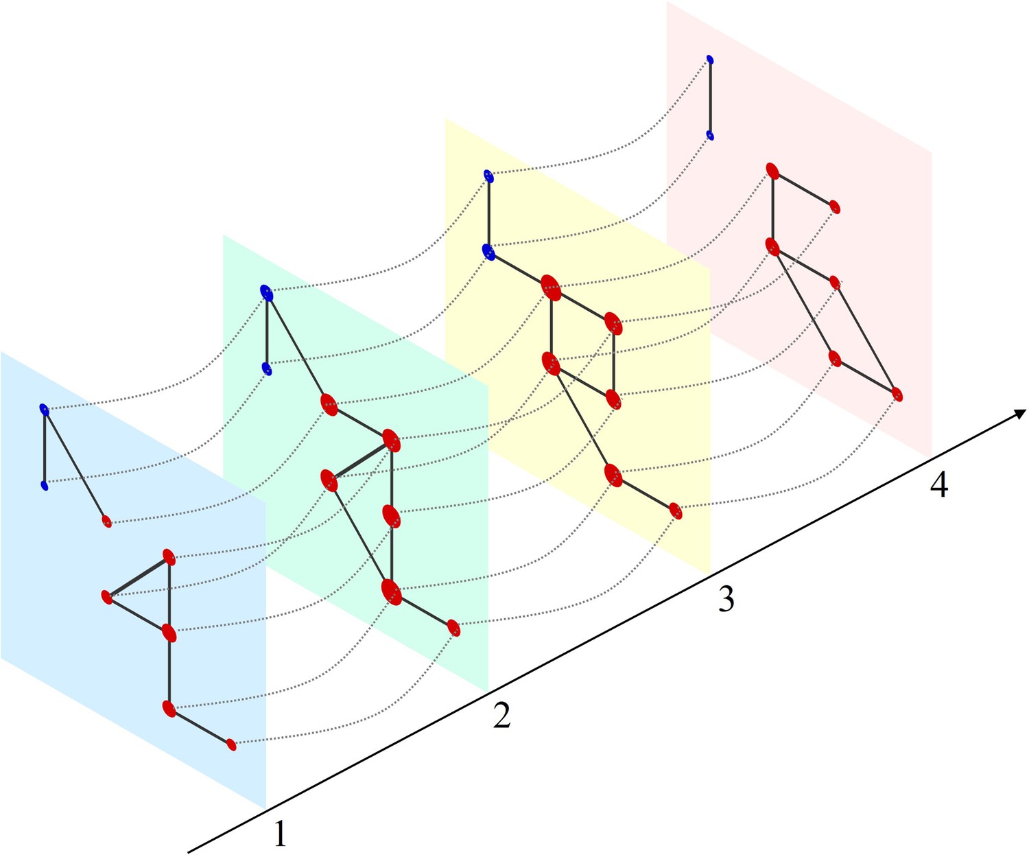
Schematic of a multilayer network and measure of multilayer eigenvector centrality (mlEVC).
Four consecutive layers (time-points) of a simulated network with intralayer (solid lines) and interlayer (dashed lines) edges. Nodes in each layer represent the set of stereoelectroencephalography (SEEG) contacts and are colored and categorized into two clusters (red and blue). Interlayer edges (couplings) were included between the same contacts at adjacent time points. The diameter of each node represents the relative value of mlEVC, in which larger nodes are the more connected nodes and smaller nodes are more isolated.
Figure 2 with 4 supplements
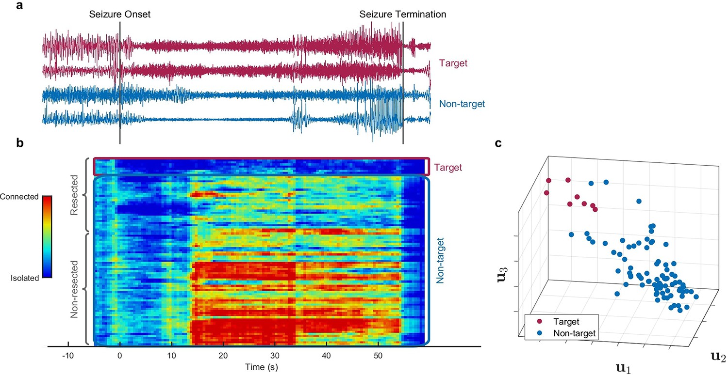
Identification of epileptogenic zone (EZ) based on multilayer eigenvector centrality (mlEVC) (Patient 17).
(a) Stereoelectroencephalography (SEEG) signals during the ictal period. The red signals are a sample of contacts inside the EZ as identified by our method, and the blue signals depict non-EZ contacts outside the resection zone. (b) The mlEVC during the ictal period. Each row represents a channel (contact). Contacts are categorized and organized into two groups: resected and non-resected as indicated on the right. They are also categorized into two groups based on the proposed clustering algorithm: target and non-target. The blue elements of mlEVC describe the isolated nodes of the super-graph (brain network) while red values describe highly connected contacts. (c) The first three left singular vectors of the mlEVC. The mlEVC spectra of different seizures were first quantized and concatenated before performing singular value decomposition. The red nodes are those identified as predicted EZ based on unsupervised clustering.
-
Figure 2—source data 1
Comparing SEEG channels identified as true positives between the two methods, mlEVC in this paper vs. those identified using the Fingerprint in Grinenko et al., 2018.
Common channels among the two methods are highlighted.
- https://cdn.elifesciences.org/articles/68531/elife-68531-fig2-data1-v2.docx
-
Figure 2—source data 2
This table summarizes the prediction performance for the proposed method and Fingerprint algorithm on 16 patients.
Important note: 16 out of 17 misidentified electrodes in our method are from three patients only.
- https://cdn.elifesciences.org/articles/68531/elife-68531-fig2-data2-v2.docx
-
Figure 2—source data 3
This table compares the prediction performance of the proposed method with a single-layer network and a multilayer network with a fixed coupling parameter for all subjects.
- https://cdn.elifesciences.org/articles/68531/elife-68531-fig2-data3-v2.docx
Figure 2—figure supplement 1
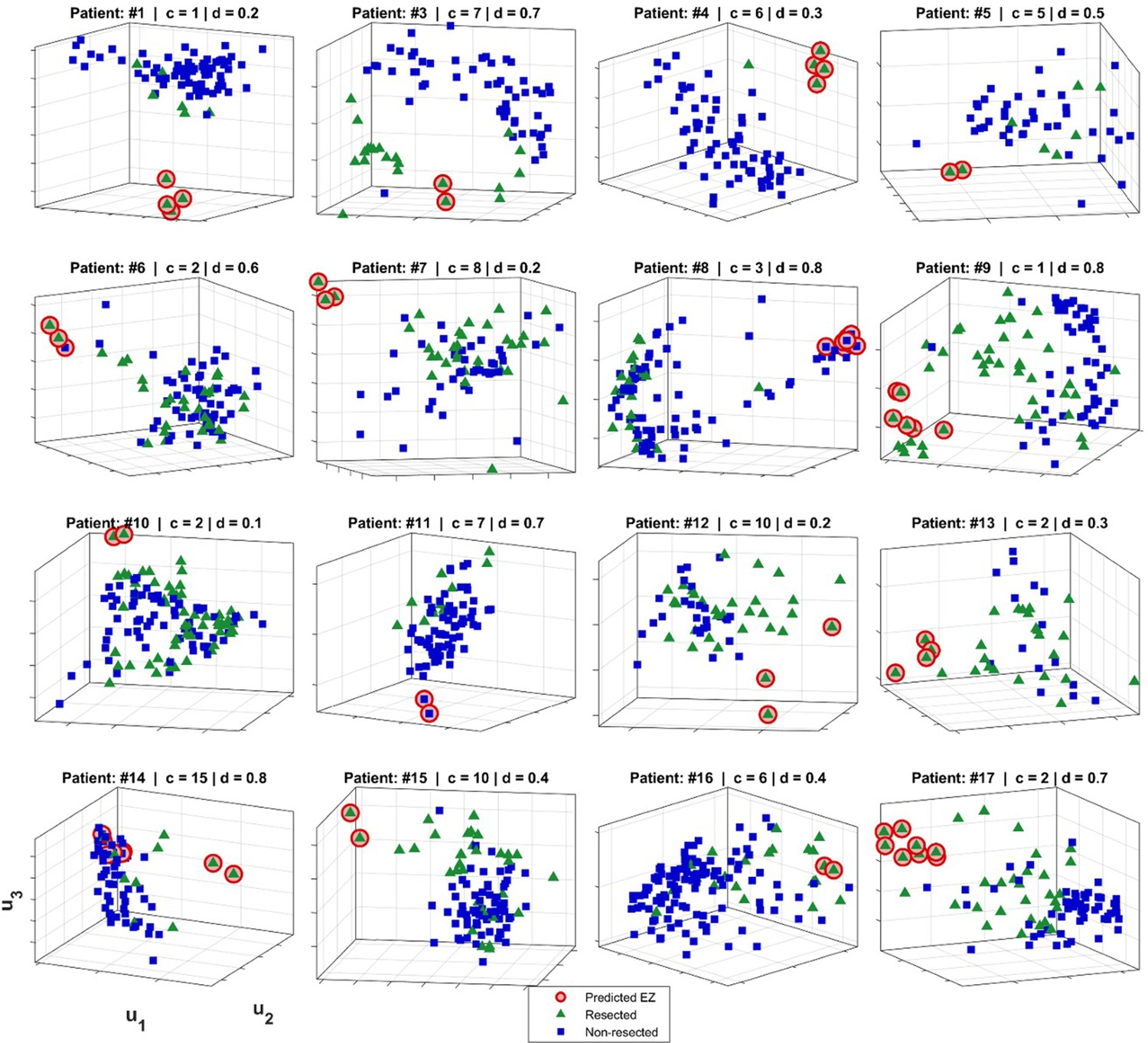
Epileptogenic zone (EZ) localization for 16 patients.
The predicted EZ (red circles) was computed as described in Methods. Blue squares show non-resected contacts and green triangles indicate the resected electrodes. The axes are the top three left singular vectors of multilayer eigenvector centrality (mlEVC), i.e., and (See Methods). For illustration purposes, we show projections with respect to the singular vectors for the parameter set (c,d) for which the prediction of EZ (binary labeling) was closest to the assumed ground truth (resection information).
Figure 2—figure supplement 2
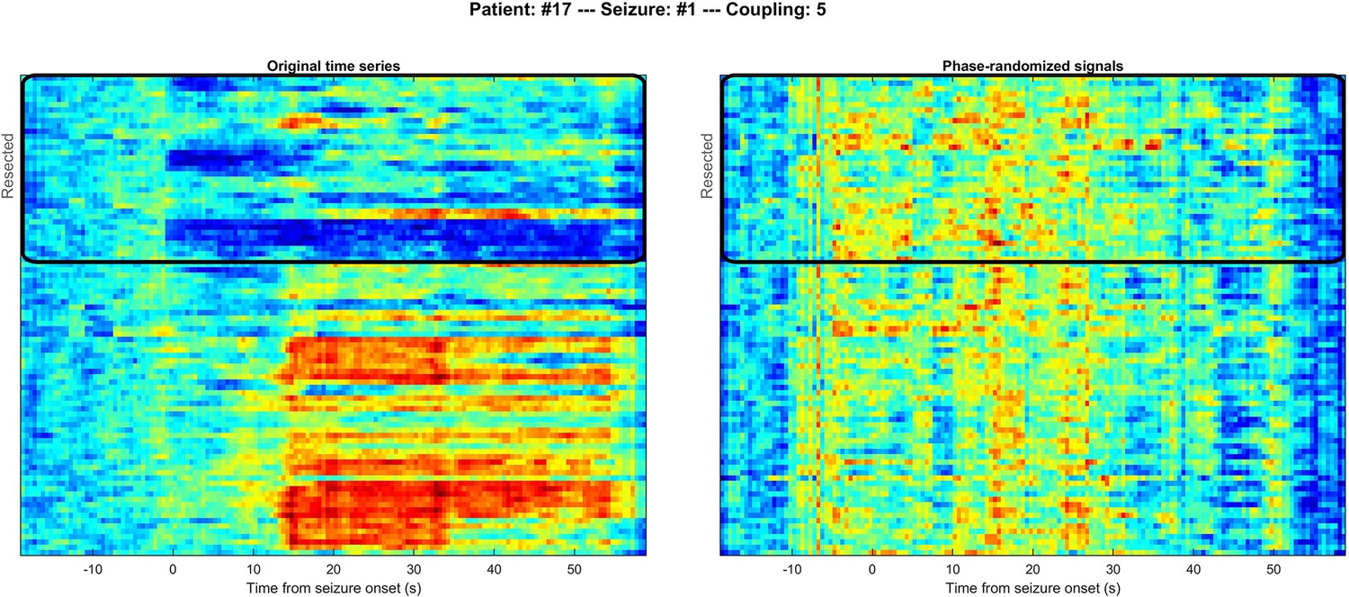
Comparison of multilayer eigenvector centrality (mlEVC) for original (left) and phase-randomized (right) seizure data for a representative subject.
Channels inside the black rectangle represent those within the resected volume as in Figure 2 in the main body of the paper. The distinction between resected and non-resected regions is lost in the phase-randomized data.
Figure 2—figure supplement 3
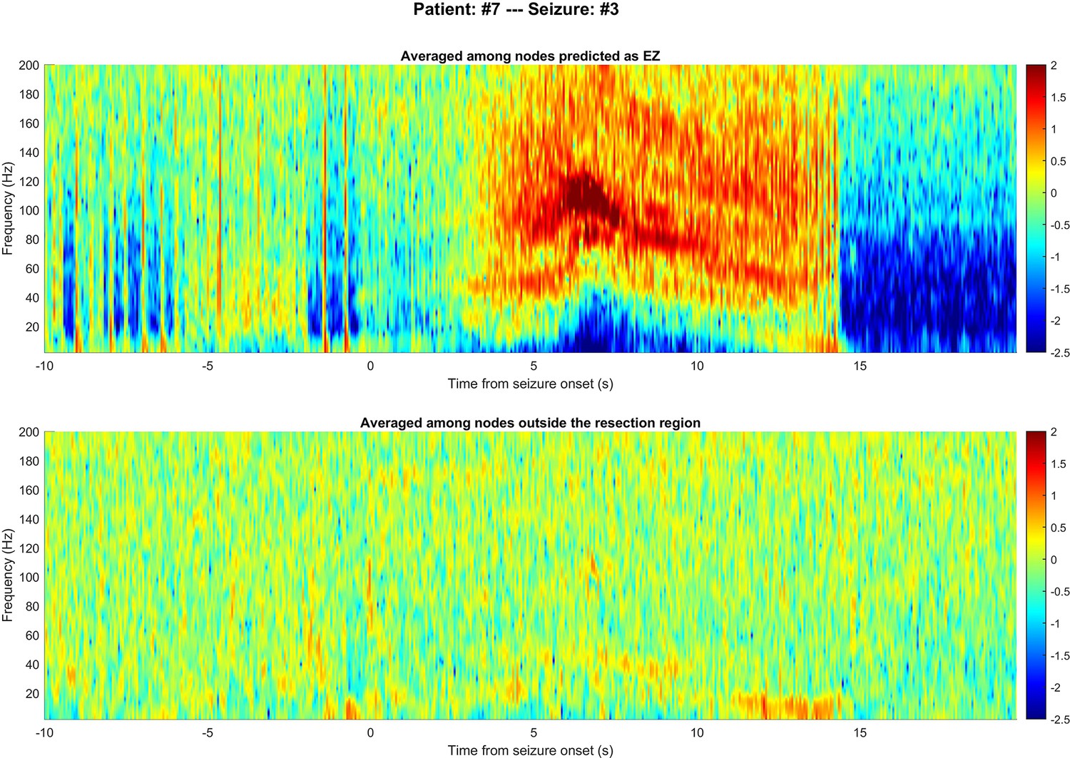
Comparing time-frequency spectrums between nodes in epileptogenic zone (EZ) and non-resected regions.
Figure 2—figure supplement 4
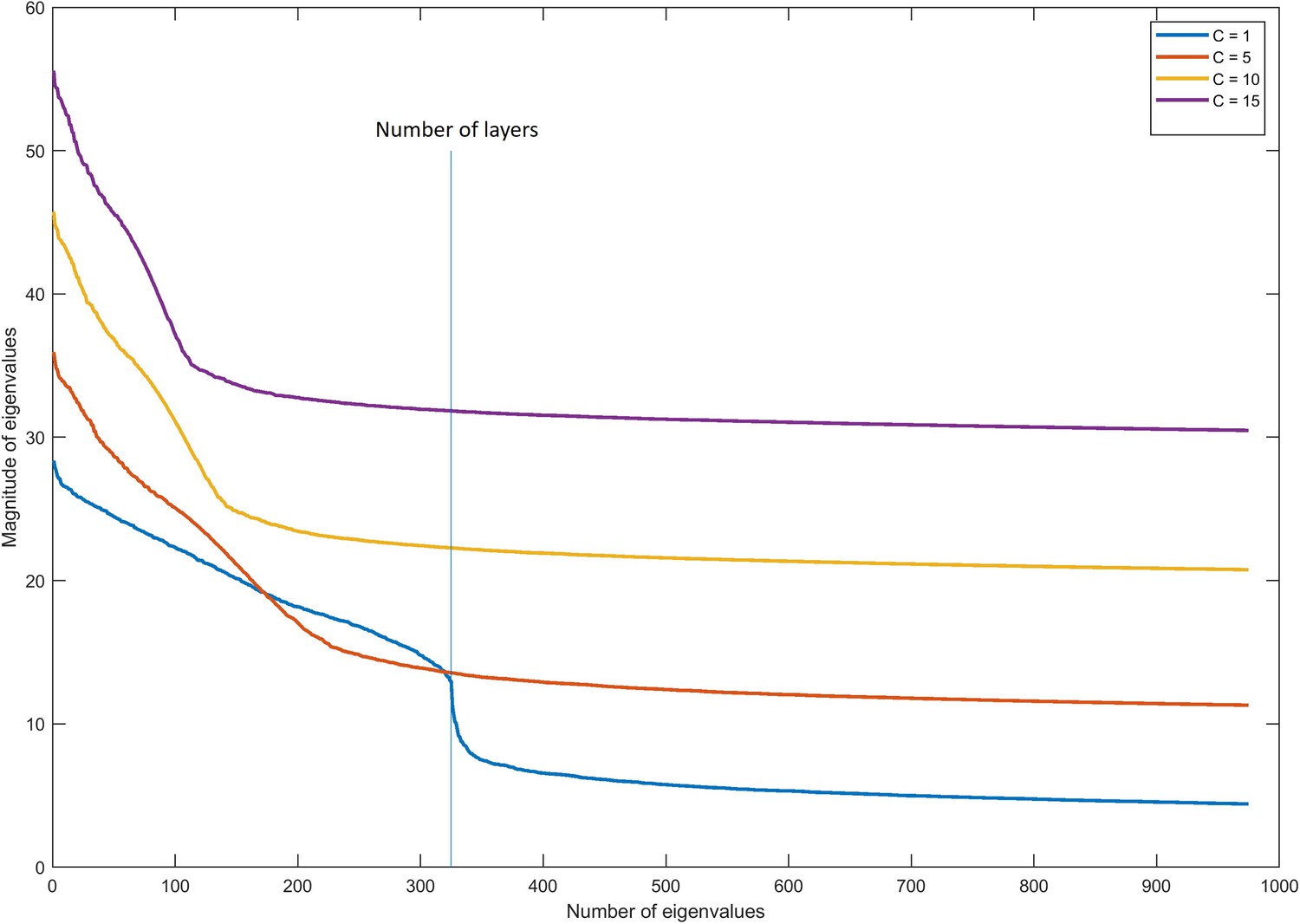
Magnitude of eigenvalues in multilayer graphs with different coupling parameters.
Figure 3 with 1 supplement
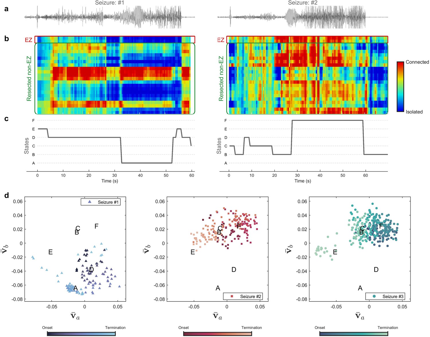
Evolution of seizures through high-frequency states (Patient 16).
(a) Time series of a channel inside the predicted epileptogenic zone (EZ) for two different seizures (onset to termination). (b) The low-rank estimation of quantized multilayer eigenvector centrality (mlEVC) plots (80–140 Hz). For a clearer representation, only channels in predicted EZ and resected non-EZ are depicted. (c) State transitions during seizures. The time vector is adjusted based on the seizure onset (t=0 s) (d) Evolution of seizures in the feature space. Capital letters show the center of each brain state. The space and states are created by four features ( , and ) extracted from the right singular vectors of mlEVC in the two high-frequency bands (see Methods – Here, only two features are illustrated). Comparing three ictal periods, we see that the brain can exhibit a different seizure evolution – here between seizure one and seizures two and three.
Figure 3—figure supplement 1
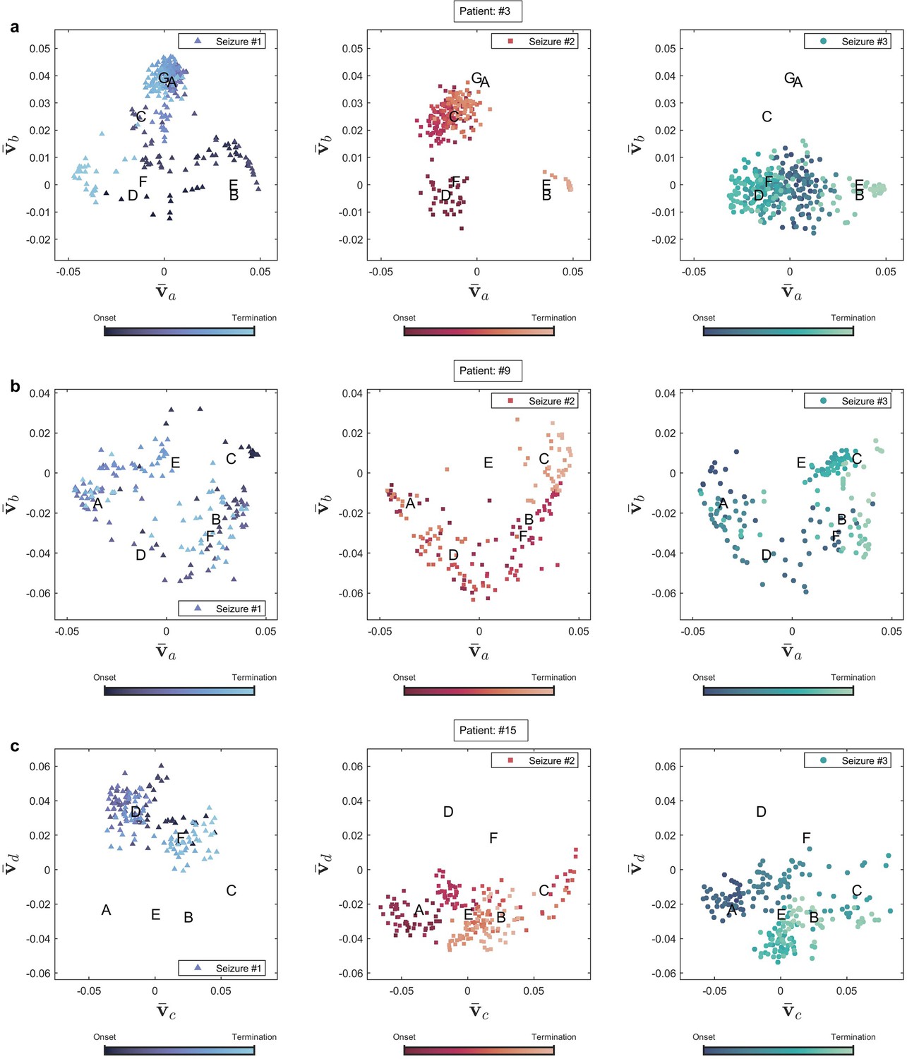
Seizure evolution and state transition in three patients.
Seizure evolution and brain states were extracted using the right singular vectors of multilayer eigenvector centrality (mlEVC) (see Methods). Capital letters show the center of each state. , and are the best features extracted from singular vectors to cluster seizure evolution into brain states. (a) Patient 3. The plot portrays states that are unique for seizures one and two, but not observed in seizure three. (b) Patient 9. All recorded seizures are scattered in the same places. (c) Patient 15. The plot depicts a distinctive area for seizure one, which was not traversed in two other reordered seizures.
Figure 4 with 1 supplement

High-frequency synchrony during the ictal period.
(a) Time-varying high-frequency synchrony values for three defined measures. The ictal period is normalized to a zero to one scale. The solid lines represent the median and shaded plots display the normalized median absolute deviation (MAD), based on 104 bootstrap tests. The gray rectangles display the periods of special interest. Note that EZ-nR connectivity drops substantially towards mid-seizure and increases to match nR-nR and RnEZ-nR at seizure termination and post-ictally. (b) Connectivity measures in pre-ictal, mid-seizure, and post-ictal. To give a pairwise visual comparison, we subtracted the average synchrony between all pairs of contacts in the pre-ictal interval from nine connectivity measures. The centers of error bars show the median of all seizures in two frequency bands and lines depict the MAD. Scatter circles exhibit the actual values (n=78 for each group). To handle possible outliers, the paired percentile bootstrap with a one-step M-estimator was employed and p-values were computed for pairwise comparison between and within the three measures at each of the three periods, corrected using Hochberg’s algorithm (B=104 number of bootstraps, J=18 tests, see Methods). Asterisks display corrected p-values; *p<0.05, **p<0.01, ***p<0.001. Only the mid-seizure interval shows significant differences between EZ-nR and other measures. All measures are considerably higher in post-ictal than their corresponding values in the mid-seizure and pre-ictal periods. EZ-nR drops significantly in mid-seizure from pre-ictal.
-
Figure 4—source data 1
Corrected p-values for all pairwise comparisons.
Post-hoc tests on network measures in high-frequency. p-values smaller than 0.05 are bolded.
- https://cdn.elifesciences.org/articles/68531/elife-68531-fig4-data1-v2.docx
Figure 4—figure supplement 1
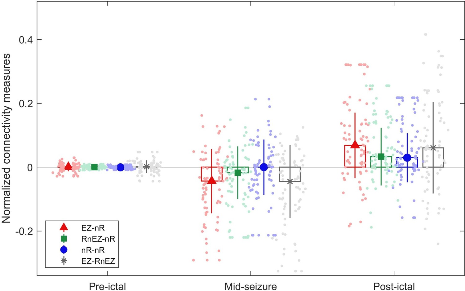
Connectivity measures in pre-ictal, mid-seizure, and post-ictal.
The center of each error bar indicates the median of all seizures (n=39) in two high-frequency bands (80–140 Hz and 140–200 Hz) and solid lines depict the scaled median absolute deviation. Scatter circles indicate the actual values (n=78 for each group). Visually, the epileptogenic zone (EZ) is strongly desynchronized with resected non-EZ.
Figure 5

Correlation between normalized EZ-nR values and patients’ history.
(a) Correlation between patients’ age and normalized EZ-nR synchronization in high frequency. Each data point indicates the average of normalized EZ-nR values in mid-seizure among two high-frequency bands for each seizure (n=39). We utilized a robust regression estimator based on bootstrap sampling and the Theil-Sen algorithm (Wilcox, 2011). (b) The same plot as (a) except where the x-axis indicates the duration of epilepsy among patients.
Figure 6

Low-frequency brain connectivity during the ictal period.
(a) Time-varying low-frequency connectivity values for three defined measures. The ictal period is normalized to a zero to one scale. The solid lines represent the median and shaded plots display the normalized median absolute deviation (MAD) based on 104 bootstrap tests. The gray rectangles display the periods of special interest. EZ-nR connectivity drops in early seizure and a widespread brain connectivity occurs in the pre-termination period. (b) Connectivity measures in pre-ictal, early-seizure, and pre-termination. To give a pairwise visual comparison, we subtracted the average synchrony between all pairs of contacts in the pre-ictal interval from nine connectivity measures. The centers of error bars show the median of all seizures in two frequency bands and lines depict the MAD. Scatter circles exhibit the actual values (n=39 for each group). To handle possible outliers, the paired percentile bootstrap with a one-step M-estimator was employed and p-values were computed for pairwise comparison between and within the three measures at each of the three periods, corrected using Hochberg’s algorithm (B=104 number of bootstraps, J=18 tests, see Methods). Asterisks display corrected p-values; *p<0.05, **p<0.01, ***p<0.001. Only the early-seizure interval shows significant differences between EZ-nR and the two other measures. All measures are considerably higher in pre-termination than their corresponding values in early-seizure and pre-ictal periods.
-
Figure 6—source data 1
Corrected p-values for all pairwise comparisons.
Post-hoc tests on network measures in low-frequency. p-values smaller than 0.05 are bolded.
- https://cdn.elifesciences.org/articles/68531/elife-68531-fig6-data1-v2.docx
Figure 7

Correlation of overall pre-termination low-frequency connectivity and post-ictal high-frequency synchrony during the critical transition.
Each point in the graph belongs to one seizure in which the two values for two high-frequency bands are averaged (n=34). Outliers were removed using the projection method and MAD-median rule (Wilcox, 2011).
Author response image 1

Magnitude and impulse response of the FIR bandpass preprocessing filter.
The upper figure shows an expanded view of the low-frequency response of the filter.
Author response image 2

Magnitude and impulse response of the notch filter.
The upper figure shows an expanded view of one of the notch bands.
Author response image 3

Time-frequency spectra and mlEVC for one seizure of patient 8.
Author response image 4

Brain state transition during three seizures of patient 15 for two coupling values.
Author response image 5

Brain state transition during three seizures of patient 3 for two coupling values.
Author response image 6
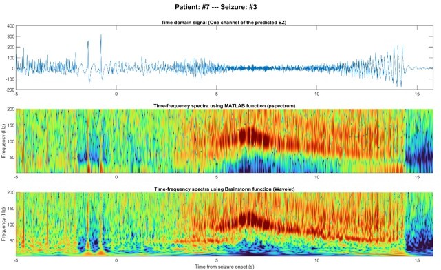
EEG signal of one node inside the predicted EZ before and after seizure onset in the time domain (top), time-frequency using MATLAB (middle), and time-frequency using Brainstorm (bottom).
Author response image 7

Pre-ictal spikes (top) and ictal HFOs (bottom) of one node inside the predicted EZ.
Tables
Table 1
Clinical characteristics of patients.
| ID | Age (years) | ED (years) | MRI lesion | Resection/ablation details | Surgical pathology | Follow-up(months) | Anatomical location of the EZ | Number of nodes in the network | Number of nodes inside the resection area | Duration of seizures (seconds) |
|---|---|---|---|---|---|---|---|---|---|---|
| 1 | 43 | 37 | FCD, insular/frontal operculum | Anterior insular/ frontal operculum | FCD type 2B | 13 | Insular/frontal operculum | 88 | 11 | (41, 39, 39) |
| 3 | 33 | 17 | Hippocampal sclerosis | Anterior temporal lobe | Hippocampal sclerosis | 48 | Temporal | 79 | 22 | (147, 150, 141) |
| 4 | 17 | 8 | Negative | Laser ablation, superior frontal gyrus | No pathology | 19 | Frontal | 71 | 5 | (25, 24, 25) |
| 5 | 16 | 1 | Benign neoplasm, posterior para-hippocampal gyrus | Posterior para- hippocampus gyrus and neoplasm | Low grade glial/ glioneuronal neoplasm | 39 | Basal posterior temporal | 48 | 8 | (55, 115, 140) |
| 6 | 46 | 41 | FCD, mesial frontal | Prefrontal lobe | Non-specific | 38 | Frontal | 88 | 32 | (100, N/D, N/D) |
| 7 | 5 | 1 | Negative | Superior frontal gyrus, superior frontal sulcus, frontal pole | FCD type 2B | 21 | Superior frontal gyrus/superior frontal sulcus | 73 | 33 | (14, 15, 15) |
| 8 | 63 | 14 | Negative | Orbitofrontal | FCD type 1 | 44 | Orbitofrontal/ pars orbitalis | 105 | 19 | (61, 267, 62) |
| 9 | 33 | 19 | Gliotic postoperative changes | Anterior temporal lobe | FCD type 1B | 40 | Temporal | 99 | 46 | (85, 64, 81) |
| 10 | 21 | 11 | Negative | Occipital lobe | Gray matter heterotopia, FCD type 1B | 12 | Cuneus | 123 | 57 | (106, 98) |
| 11 | 32 | 27 | FCD, precentral gyrus | Precentral gyrus | Non-conclusive | 77 | Precentral gyrus | 82 | 13 | (26, 78, 12) |
| 12 | 22 | 3 | FCD, superior frontal sulcus | Superior and middle frontal gyri, anterior cingulate | FCD type 2B | 78 | Frontal | 58 | 31 | (18, 25, 31) |
| 13 | 19 | 18 | Negative | Middle frontal gyrus | FCD type 1 | 48 | Inferior frontal sulcus/middle frontal gyrus | 41 | 26 | (36, 36, 35) |
| 14 | 30 | 18 | Negative | Frontal operculum | FCD type 2B | 47 | Frontal operculum/ subcentral region | 70 | 10 | (49, 21, 78) |
| 15 | 20 | 11 | Negative | Frontal lobe | FCD type 1 | 82 | Superior frontal gyrus/superior frontal sulcus | 99 | 32 | (65, 86, 86) |
| 16 | 65 | 25 | Negative | Anterior temporal lobe | FCD type 1 C | 39 | Temporal | 139 | 23 | (56, 65, 142) |
| 17 | 65 | 9 | Negative | Anterior temporal lobe | FCD type 1 C | 36 | Temporal | 90 | 35 | (55, 63, 59) |
-
Follow-up information is current as of July 2017.
-
ED: epilepsy duration, FCD: focal cortical dysplasia, N/D: Not defined.
Additional files
Download links
A two-part list of links to download the article, or parts of the article, in various formats.
Downloads (link to download the article as PDF)
Open citations (links to open the citations from this article in various online reference manager services)
Cite this article (links to download the citations from this article in formats compatible with various reference manager tools)
Multilayer brain networks can identify the epileptogenic zone and seizure dynamics
eLife 12:e68531.
https://doi.org/10.7554/eLife.68531


