A state space modeling approach to real-time phase estimation
- Mathematics and Statistics, Boston University, United States
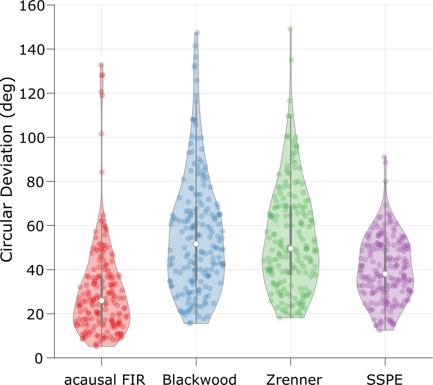
- Department of Psychiatry, University of Minnesota, United States
- Center for Systems Neuroscience, Boston University, United States
Figures
Figure 1
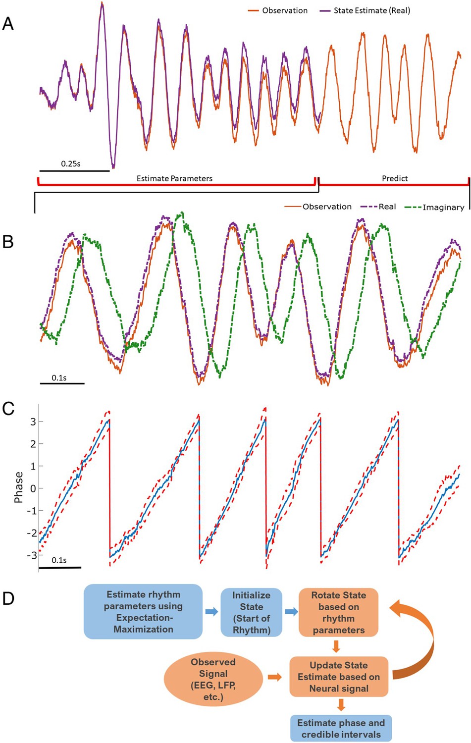
Illustration of state space phase estimate (SSPE) procedure.
Given an observation (A, red), we estimate model parameters in an initial interval of data. At subsequent times, we use the observed data to (B) predict and update the state estimate (purple), and (C) the phase and credible intervals, causally estimated. Note that prediction can be done for any time after parameter estimation; here we show a representative time interval. (D) Conceptual diagram of the steps involved in the SSPE method.
Figure 2
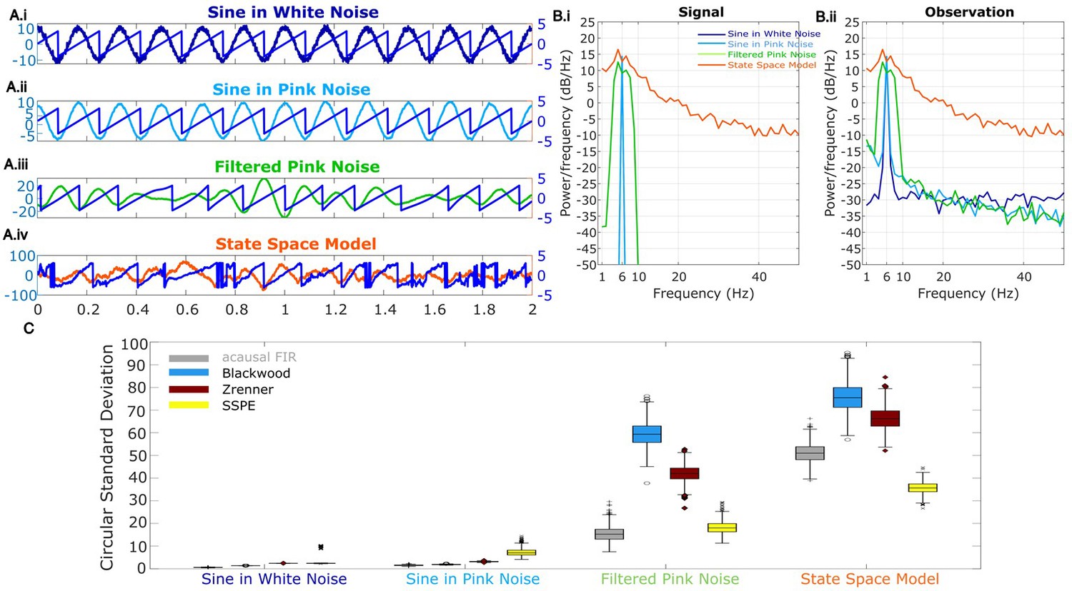
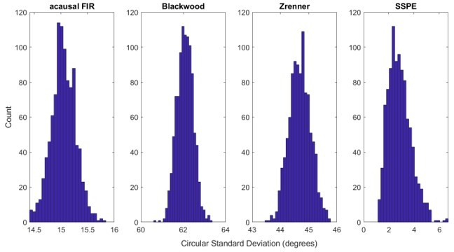
Wide band rhythm’s phase better tracked with state space phase estimate (SSPE).
(A) Example 2 s of simulated observed data (thick curves) and the true phase (thin blue curves) for each scenario. (B) For each scenario, example spectra of (B.i) the signal, and (B.ii) the observation (i.e., signal plus noise). Spectra were estimated for 10 s segments using the function ‘pmtm’ in MATLAB, to compute a multitaper estimate with frequency resolution 1 Hz and nine tapers. (C) The phase error for each estimation method (see legend) and simulation scenario. In each box plot, the central mark indicates the median; the bottom and top edges of the box indicate the 25th and 75th percentiles, respectively; the whiskers indicate the most extreme data points not considered outliers.
-
Figure 2—source data 1
Circular standard deviation for all methods.
- https://cdn.elifesciences.org/articles/68803/elife-68803-fig2-data1-v2.mat
Figure 3
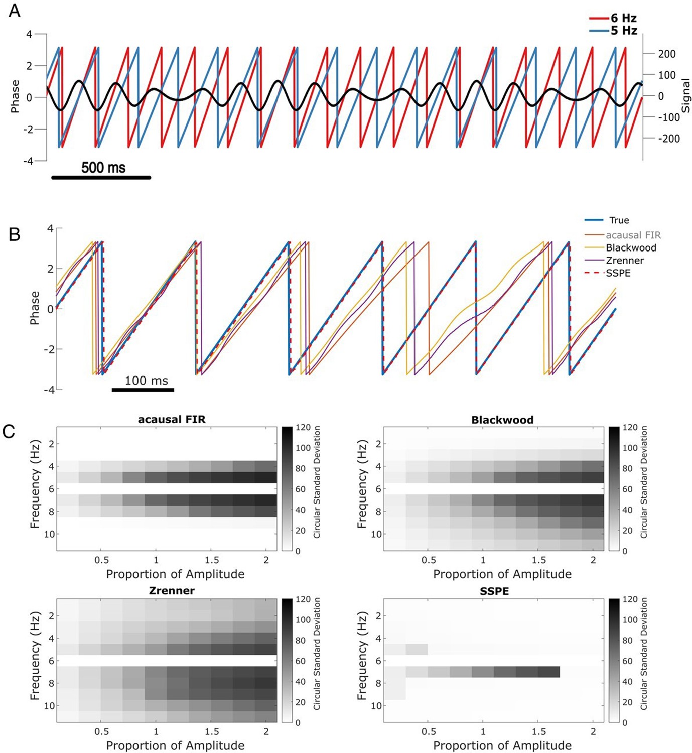
SSPE performs well when two oscillations exist at nearby frequencies.
(A) Example observed signal (black) and phase for two simulated rhythms, the confounding rhythm at 5 Hz (blue) and the target rhythm at 6 Hz (red). (B) Example phase estimates for the target rhythm in (A) using four different approaches (see legend). (C) Estimation error (circular standard deviation, see scale bars) for each estimation method as a function of frequency and amplitude of the confounding oscillation. In all cases the error increases as the frequency of the confounding oscillation approaches 6 Hz (the frequency of the target oscillation), and as the amplitude of the confounding oscillation increases.
-
Figure 3—source data 1
Circular standard deviation for all methods on two simultaneous oscillations simulation.
- https://cdn.elifesciences.org/articles/68803/elife-68803-fig3-data1-v2.mat
Figure 4
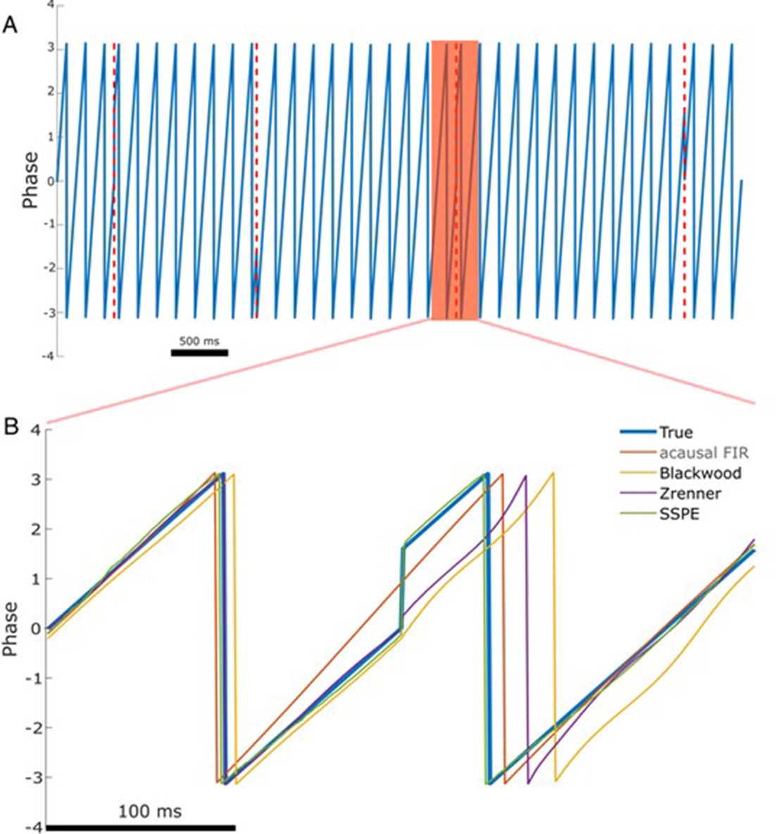
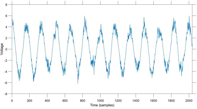
The state space phase estimate (SSPE) accurately tracks phase following a phase reset.
(A) Example phase of a 6 Hz sinusoid (blue) with four phase resets (red dashed lines). (B) Example phase estimates (thin curves) and the true phase (thick blue curve) at the indicated phase reset in (A). The SSPE method (in green) tracks the true phase much more closely than other methods following a phase reset.
Figure 5 with 1 supplement
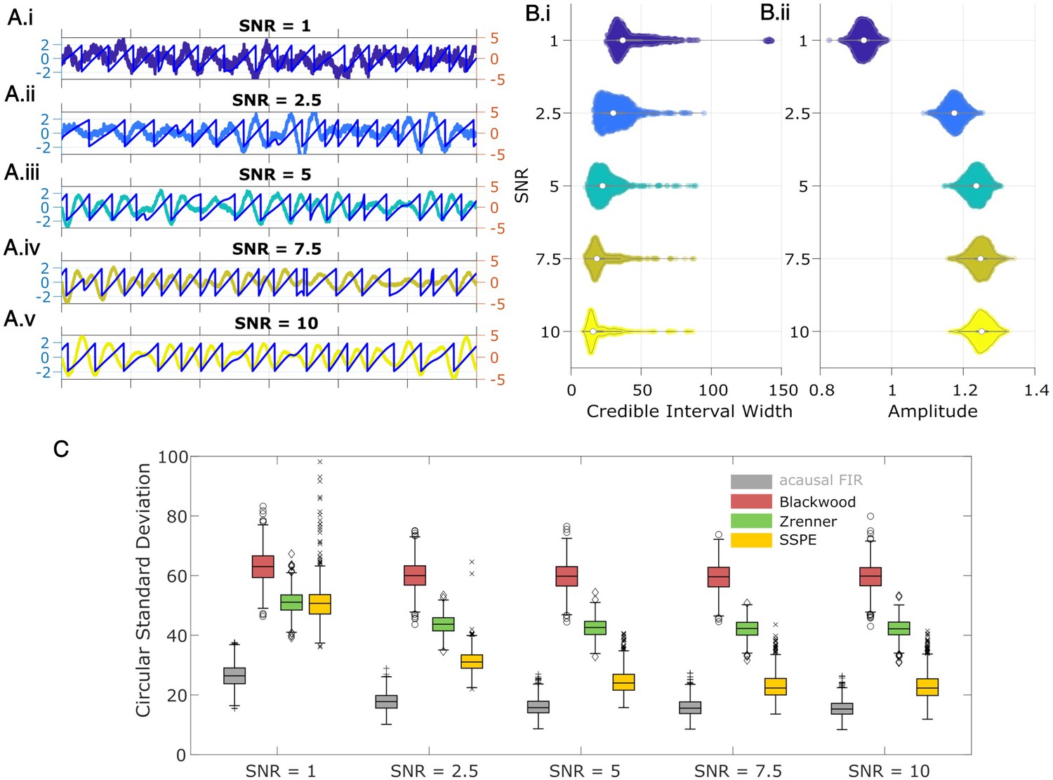
State space phase estimate (SSPE) tracks an oscillatory signal with less error across a range of signal-to-noise ratios (SNR).
(A) Example 2 s of simulated observed data (thick curves) and true phase (thin blue curves) for each SNR value. (B) For each SNR, (i) the average credible interval width (colored circles) of the SSPE method for all simulation iterations, and (ii) the average amplitude of the estimated signal (colored circles) for all simulation iterations. White circles (horizontal gray lines) indicate median (25th and 75th percentiles) values for each SNR. (C) The phase error for each estimation method (see legend) and simulation SNR. In each box plot, the central mark indicates the median; the bottom and top edges of the box indicate the 25th and 75th percentiles, respectively; the whiskers indicate the most extreme data points not considered outliers.
-
Figure 5—source data 1
Circular standard deviation for all methods on signal-to-noise ratio (SNR) simulation.
- https://cdn.elifesciences.org/articles/68803/elife-68803-fig5-data1-v2.mat
Figure 5—figure supplement 1
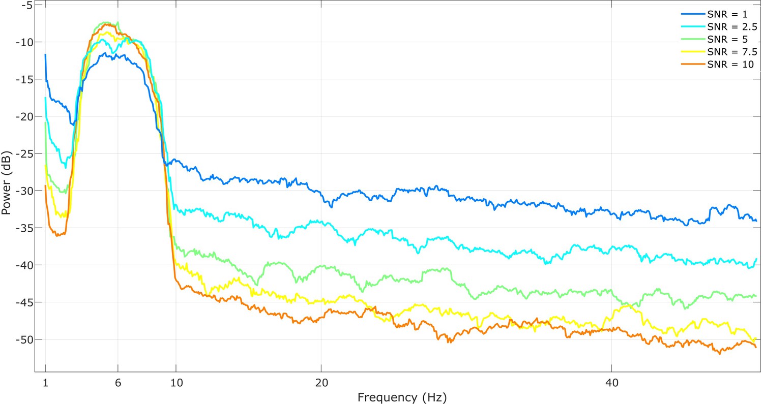
Example power spectra for all simulated cases.
At each signal-to-noise ratio (SNR), for a smooth spectrum, we used 15 s of data and applied the multitaper method with 29 tapers and a bandwidth of 1 Hz. The SNR is controlled by shifting the power of the signal relative to the pink noise, demonstrated by the changing height of the peak at 6 Hz above the noise.
Figure 6 with 1 supplement
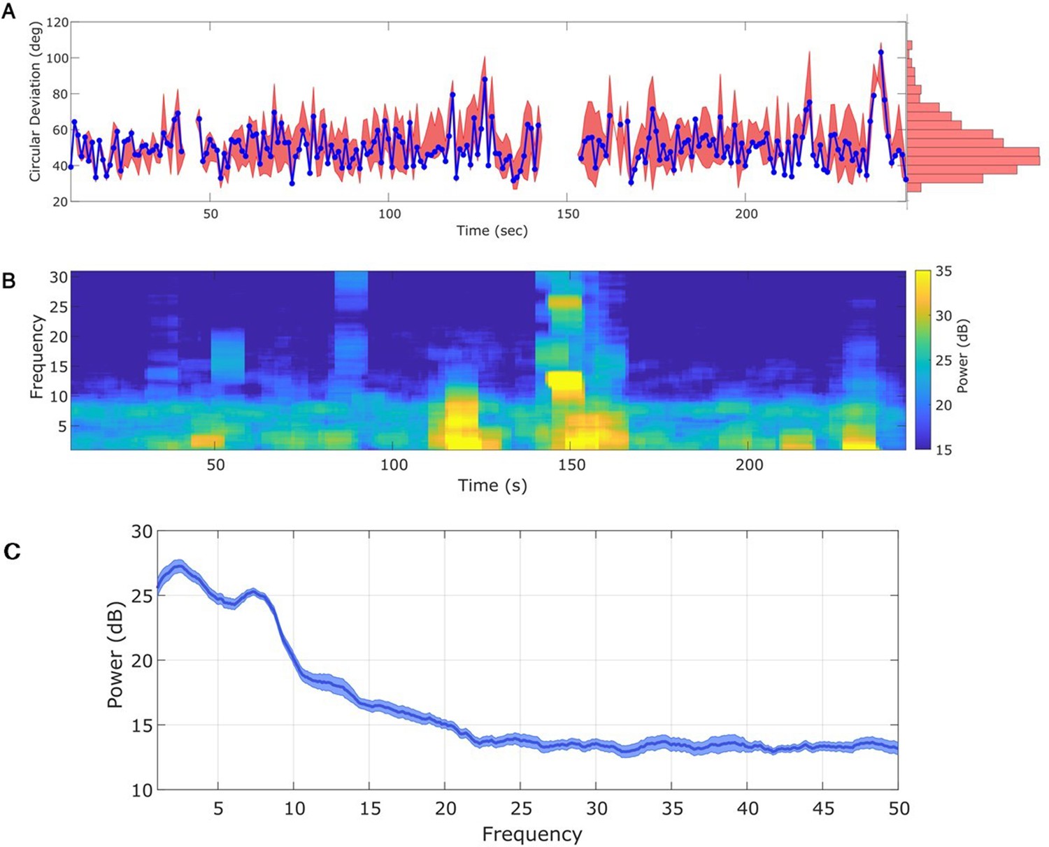
Any interval with a prominent rhythm of interest (here: theta) can be used to fit state space phase estimate (SSPE) parameters.
(A) The phase error for a single instance of the model fit (using data at times 10–20 s, blue curve), and the 90% interval for phase error (red bands) at time t derived using parameter estimates from all models estimated with data prior to t. The moments where no error is reported are moments when an acausal approach failed to detect the theta band rhythm. Right: a histogram of circular deviation across all time demonstrating that error remains below 60 degrees in the majority of cases. (B) Corresponding spectrogram of the rodent local field potential (LFP) data (multitaper method with window size 10 s, window overlap 9 s, frequency resolution 2 Hz, and 19 tapers). (C) Average power spectral density (PSD) of (B) over all times with theta band oscillator identified in (A). The mean PSD (dark blue) and 95% confidence intervals (light blue) reveal a broadband peak in the theta band.
-
Figure 6—source data 1
Error and spectrogram for in vivo local field potential (LFP) data.
- https://cdn.elifesciences.org/articles/68803/elife-68803-fig6-data1-v2.mat
Figure 6—figure supplement 1
The state space phase estimate (SSPE) method performs optimally across algorithms when tracking local field potential (LFP) theta.
The error (circular deviation) in performance of each algorithm across all LFP data. Each dot represents the error computed for 1 s of data. To compute the error, we compare the real-time phase estimate of each method to an acausally derived estimate of the phase by fitting the state space model (see Materials and methods: In vivo data). The SSPE method shows performance comparable to the acausal finite impulse response (FIR).
Figure 7 with 1 supplement
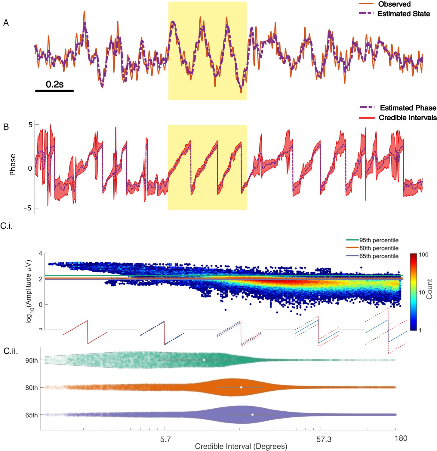
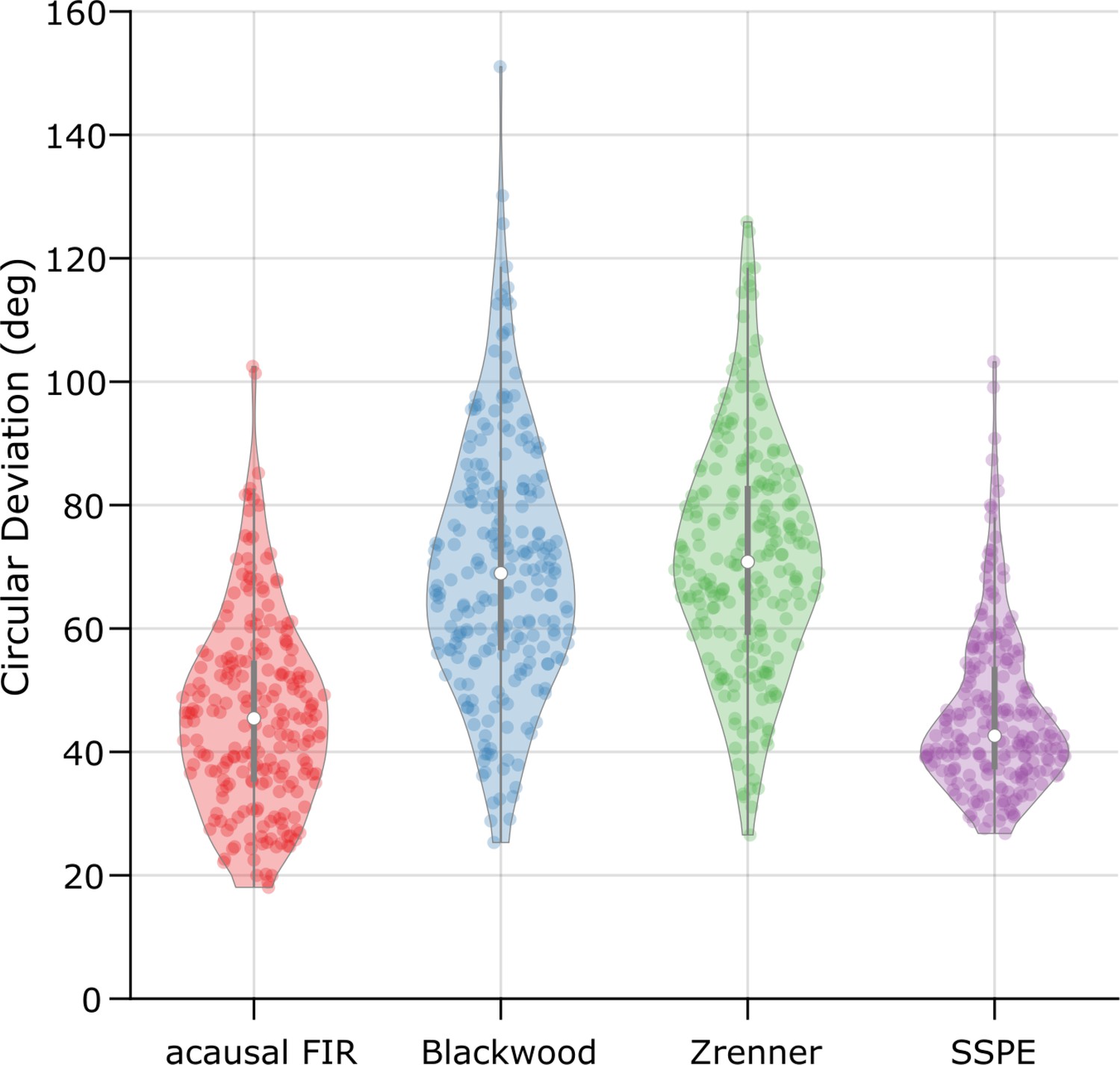
State space phase estimate (SSPE) tracks in vivo credible intervals for the phase.
(A) Example rodent local field potential (LFP) data (red, solid) with a consistent broadband peak in the theta band (4–8 Hz). The estimated state of the SSPE method (purple, dashed) tracks the observed LFP. (B) Phase estimates (purple, dashed) and credible intervals (red, shaded) for the example LFP data in (A). When the rhythm appears (yellow shaded region) the credible intervals approach the mean phase; when the rhythm drops out, the credible intervals expand. (C.i) Phase credible intervals versus theta rhythm amplitude for each time point shown as a two-dimensional histogram (color indicates count of time points; see colorbar). (Lower) Example cycles of a rhythm with credible intervals, see x-axis of (C.ii) for numerical values of credible intervals. (C.ii) Violin plot of credible intervals for thresholds set at the 65th, 80th, and 95th percentile of the distribution of amplitude. The distribution of credible intervals increases with reduced amplitude threshold, and all amplitude thresholds include times with large credible intervals. Note that the phase and amplitude estimates are auto-correlated in time so that each gray dot is not independent of every other dot.
-
Figure 7—source data 1
Amplitude and credible interval widths for local field potential (LFP) data.
- https://cdn.elifesciences.org/articles/68803/elife-68803-fig7-data1-v2.mat
Figure 7—figure supplement 1
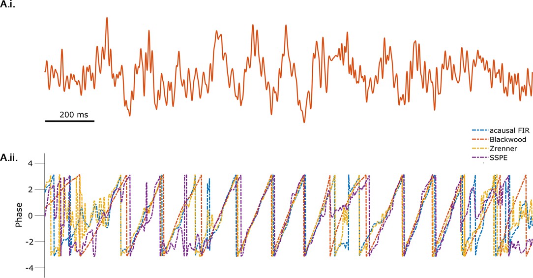
All methods produce similar phase estimates during segments of the theta rhythm with high signal-to-noise ratio (SNR).
(A.i.) Example rodent local field potential (LFP) data. (A.ii) Phase estimates from each method (see legend) are consistent when the SNR of the theta rhythm is high.
Figure 8 with 3 supplements
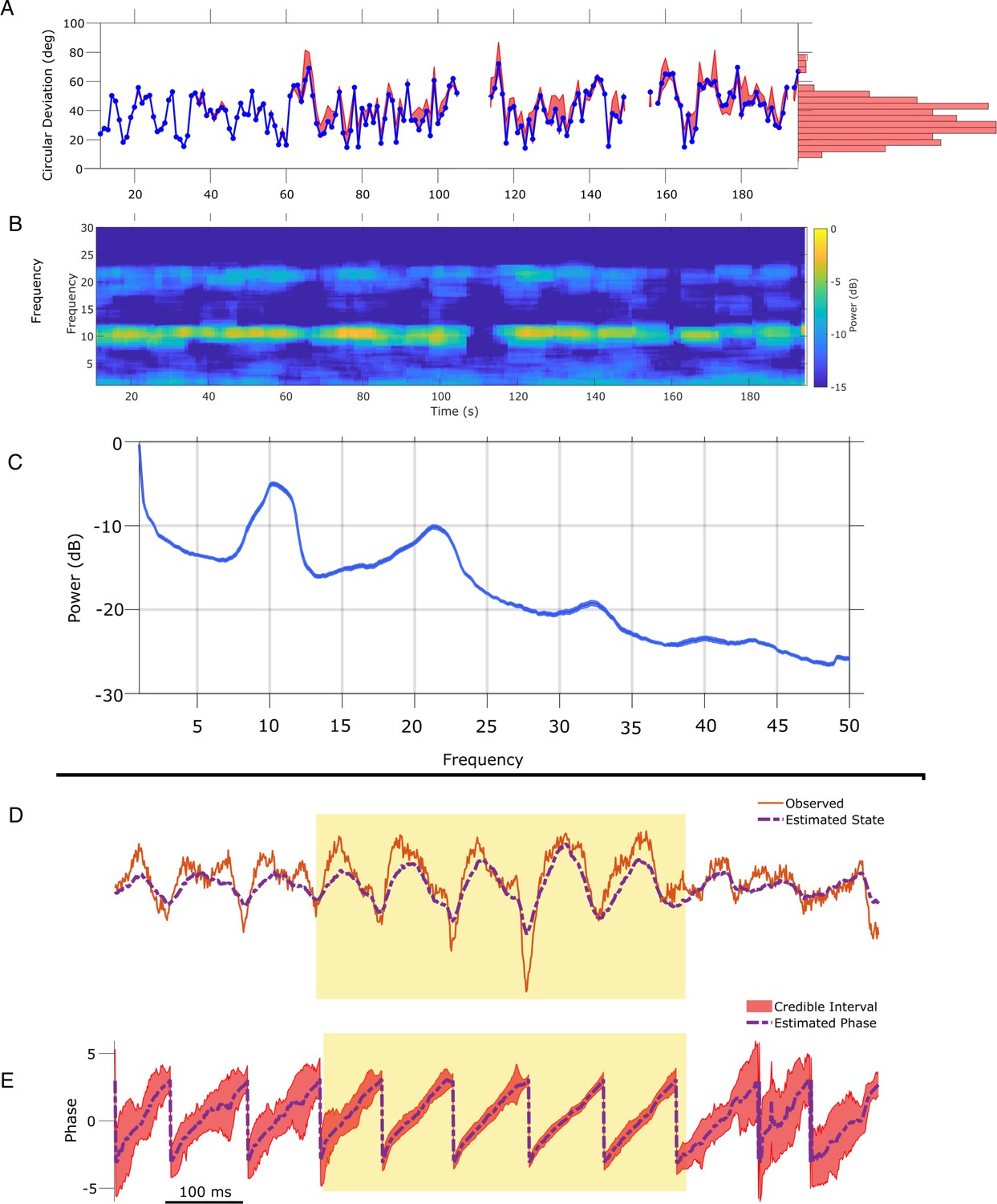
State space phase estimate (SSPE) parameters can be estimated from any interval of electroencephalogram (EEG) mu rhythm and credible intervals for mu rhythm phase indicate periods of confidence.
(A) Phase error for a model fit using data from the first 10 s (blue curve), and the 95% confidence intervals (red) in the error for phase estimates at time t using models fit at times prior to time t. Right: histogram of error showing that error remains below 60 degrees in most cases. (B) Corresponding spectrogram for the EEG data (multitaper method with window size 10 s, window overlap 9 s, frequency resolution 1 Hz, and 19 tapers). (C) Average power spectral density (PSD) of (B) over all times in (A). The mean PSD (dark blue) and 95% confidence intervals (light blue) reveal a peak in the mu rhythm near 11 Hz. (D) Example human EEG data (red, solid) with a consistent peak in the mu rhythm (8–13 Hz). The estimated state of the SSPE method (purple, dashed) tracks the observed mu rhythm. (E) Phase estimates (purple, dashed) and credible intervals (red, shaded) for the example EEG data in D. When the rhythm appears (yellow shaded region) credible intervals approach the mean phase; when the rhythm drops out the credible intervals expand.
-
Figure 8—source data 1
Error and spectrogram for in vivo electroencephalogram (EEG) analysis.
- https://cdn.elifesciences.org/articles/68803/elife-68803-fig8-data1-v2.mat
Figure 8—figure supplement 1
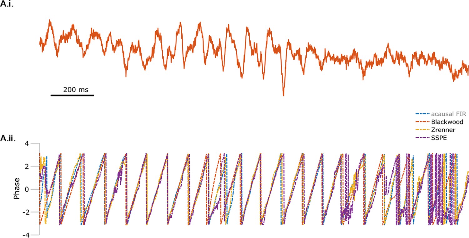
All methods produce similar phase estimates during segments of the mu rhythm with high signal-to-noise ratio (SNR).
(A.i) Example mu rhythm clearly visible in the early portion of the electroencephalogram (EEG) trace. (A.ii) Phase estimates from each method (see legend) are consistent when the SNR of the mu rhythm is high.
Figure 8—figure supplement 2
The state space phase estimate (SSPE) method performs optimally across algorithms when tracking the electroencephalogram (EEG) mu rhythm.
The error (circular deviation) in performance of each algorithm across all EEG data. Each dot represents the error computed for 1 s of data. To compute the error, we compare the real-time phase estimate of each method to an acausally derived estimate of the phase by fitting the state space model (see Materials and methods: In vivo data). The SSPE method shows performance comparable to the acausal finite impulse response (FIR).
Figure 8—figure supplement 3
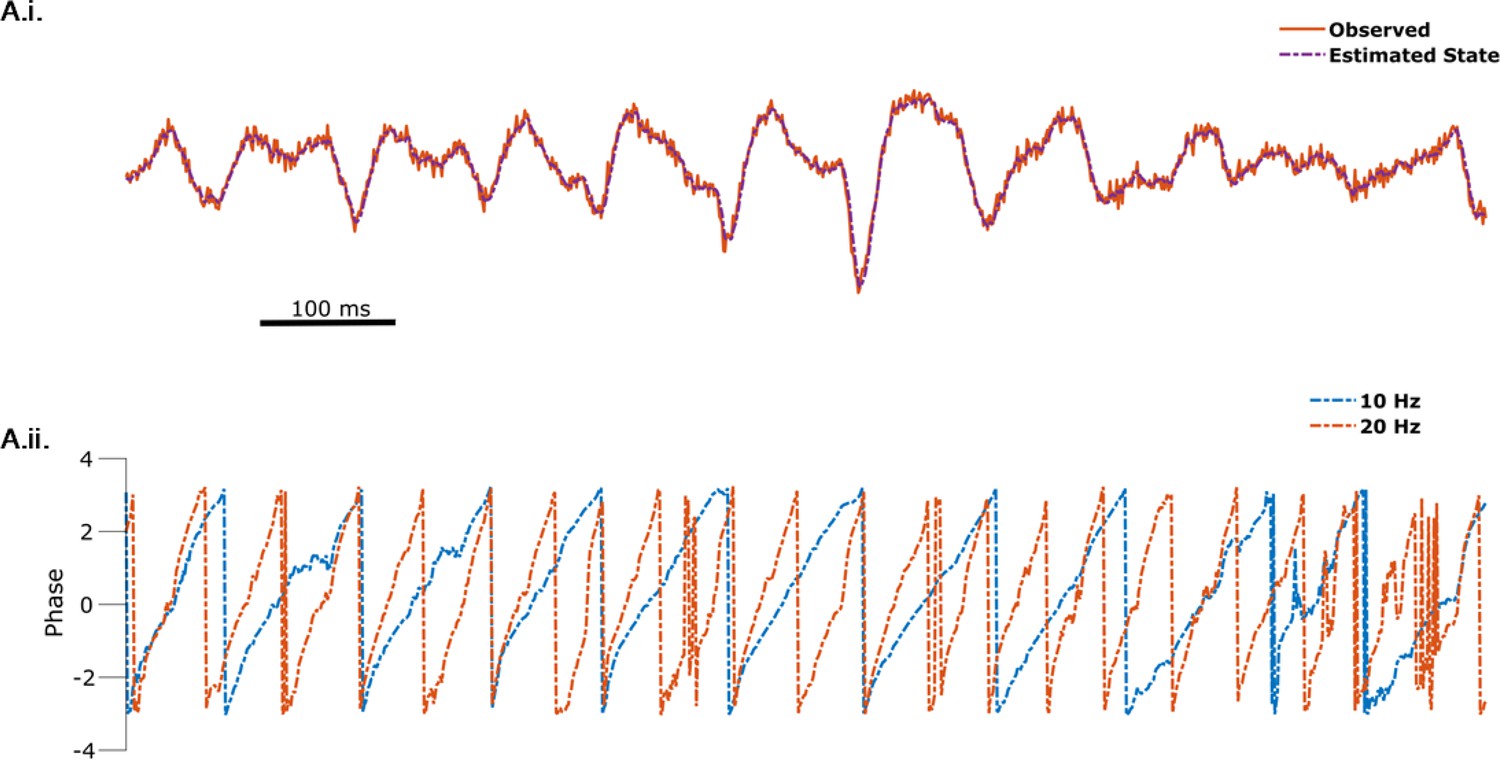
State space phase estimate (SSPE) captures non-sinusoidality of the mu rhythm.
(A.i) The observed data (orange) is well tracked by the (summed) state estimate (purple, dotted) of the 10 and 22 Hz oscillators. (A.ii) Phase estimates for the 10 Hz (blue, dotted) and 20 Hz (orange, dotted) oscillators are tracked simultaneously.
Figure 9
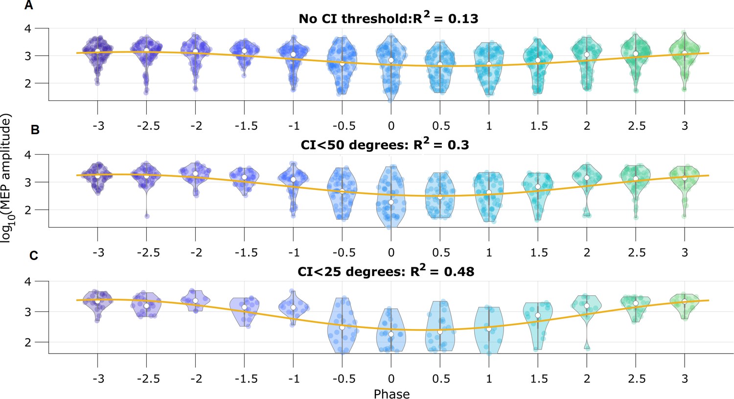
Motor evoked potential (MEP) amplitude is predicted by the pre-stimulus state space phase estimate (SSPE) estimated mu rhythm phase.
(A) Log-transformed MEP amplitude versus phase with no threshold applied to the credible interval width. White dot indicates the median of the MEP amplitude. Yellow line is the best fit circular linear regression line (a phase offset sinusoid) showing that the MEP amplitude is maximum at mu rhythm trough (phase = ±π). (B,C) Including only trials with CI width (B) less than 50 degrees, or (C) less than 25 degrees more clearly demonstrates the MEP amplitude maxima at the mu rhythm trough.
Figure 10
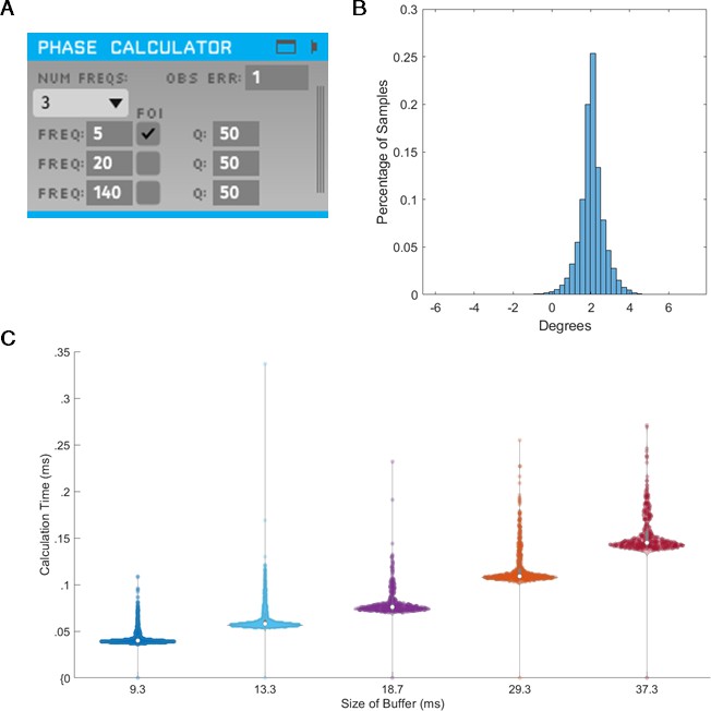
State space phase estimate (SSPE) implementation in Toolkit for Oscillatory Real-time Tracking and Estimation (TORTE) is accurate, with negligible latency.
(A) Open Ephys GUI for using SSPE. The user specifies the number of frequencies to track, the center frequencies to track, the frequencies of interest for phase calculation and output (FOI), variance for the FOI, and the observation error. Observation error determines the effective bandwidth for each frequency. (B) Histogram of the circular standard deviation between MATLAB (offline) and TORTE (real-time) implementations of the SSPE. Small variation results from causal low pass filtering in TORTE and acausal filtering in the offline phase estimates. (C) Time to evaluate phase versus buffer size. Longer buffer sizes from TORTE require longer calculation time for application of SSPE. However, the calculation time is approximately two orders of magnitude smaller than the buffer size.
Author response image 1

Author response image 2
Author response image 3

The SSPE method performs as well as the acausal FIR and Blackwood methods for 1/f amplitude modulated data.
Author response image 4
Author response image 5
Author response image 6
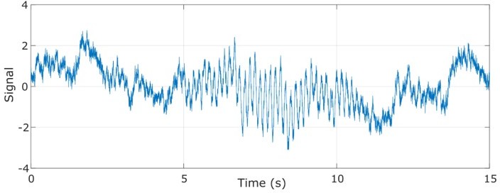
Example data trace for the proposed model.
The amplitude of the 6 Hz sinusoid waxes and wanes in time.
Author response image 7

The Blackwood method outperforms the other causal algorithms for the multiplicative 1/f sinusoid example, similar to “Sines in Pink Noise”.
Author response image 8

.
We find that SSPE still performs well for two oscillations at nearby frequencies, with random initial phases; compare to Figure 3 of the main manuscript.
Author response image 9
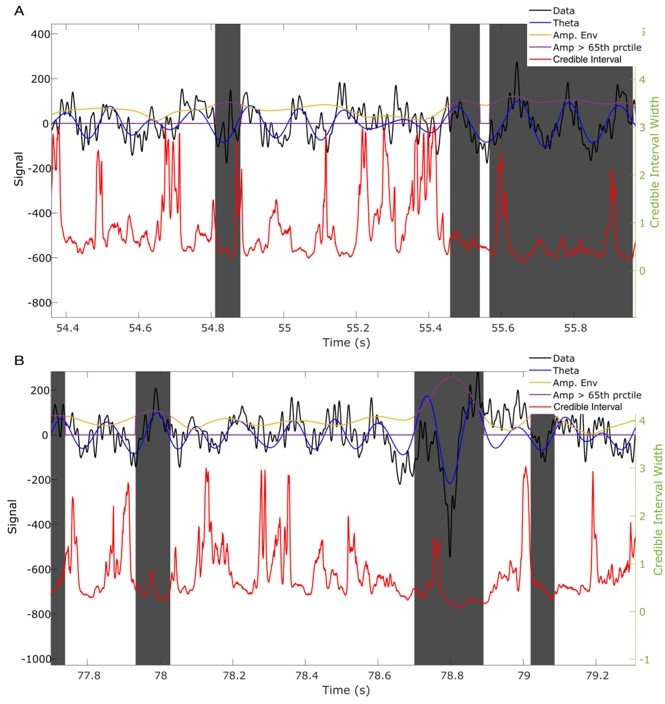
Credible intervals better capture the presence of theta cycles than an amplitude threshold.
(A,B) Two example traces showing intervals in which the rhythm amplitude is small (below the 65th percentile, white intervals, also indicated by purple trace equaling 0), yet the credible intervals suggest confidence in the phase estimate, consistent with the presence of a theta rhythm. Visual inspection of data filtered (4 – 11 Hz FIR filter, blue curve) in the theta band suggests the presence of a theta rhythm. Gray intervals indicate periods of high amplitude (above the 65th percentile). In these intervals there exist periods with wide credible intervals (at times when the SSPE method is uncertain if the rhythm is rising or falling) suggesting a simple amplitude threshold is insufficient to determine confidence in the phase estimates.
Tables
Table 1
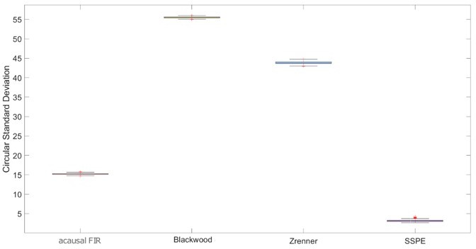
Error following phase reset for different phase estimation methods.
| SSPE | Blackwood | Zrenner | Acausal FIR | |
|---|---|---|---|---|
| Error (std. dev.) | 2.85 (0.89)* | 62.08 (0.38) | 44.68 (0.38) | 15.04 (0.23) |
| Time to convergence(std. dev.) | 34 ms (162) | 190 ms (33) | 747 ms (22) | 555 ms (206) |
-
*
p~0 compared to all other methods.
-
Table 1—source data 1
Circular standard deviation and convergence time information for phase reset simulation.
- https://cdn.elifesciences.org/articles/68803/elife-68803-table1-data1-v2.zip
Additional files
Download links
A two-part list of links to download the article, or parts of the article, in various formats.
Downloads (link to download the article as PDF)
Open citations (links to open the citations from this article in various online reference manager services)
Cite this article (links to download the citations from this article in formats compatible with various reference manager tools)
A state space modeling approach to real-time phase estimation
eLife 10:e68803.
https://doi.org/10.7554/eLife.68803


