Fast and accurate annotation of acoustic signals with deep neural networks
- European Neuroscience Institute - A Joint Initiative of the University Medical Center Göttingen and the Max-Planck-Society, Germany
- International Max Planck Research School and Göttingen Graduate School for Neurosciences, Biophysics, and Molecular Biosciences (GGNB) at the University of Göttingen, Germany
- Bernstein Center for Computational Neuroscience, Germany
Figures
Figure 1 with 3 supplements
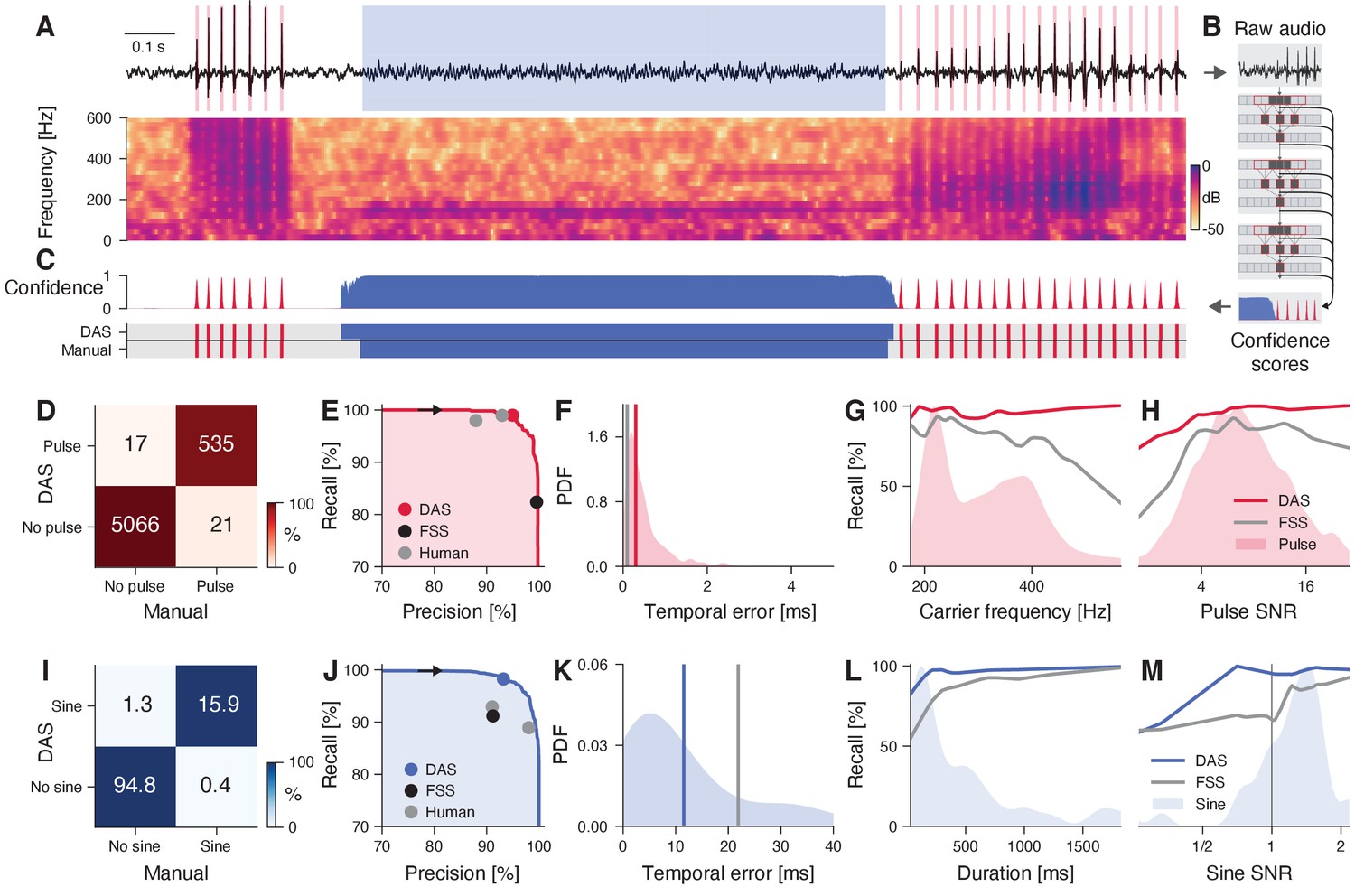
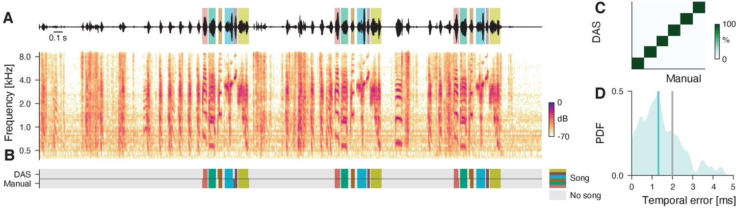
DAS performance for fly song.
(A) Fly song (black, top) with manual annotations of sine (blue) and pulse (red) song. The spectrogram (bottom) shows the signal’s frequency content over time (see color bar). (B) DAS builds a hierarchical presentation of song features relevant for annotation using a deep neural network. The network consists of three TCN blocks, which extract song features at multiple timescales. The output of the network is a confidence score for each sample and song type. (C) Confidence scores (top) for sine (blue) and pulse (red) for the signal in A. The confidence is transformed into annotation labels (bottom) based on a confidence threshold (0.5 for sine, 0.7 for pulse). Ground truth (bottom) from manual annotations shown for comparison. (D) Confusion matrix for pulse from the test data set. Color indicates the percentage (see color bar) and text labels indicate the number of pulses for each quadrant. All confusion matrices are normalized such that columns sum to 100%. The concentration of values along the diagonal indicates high annotation performance. (E) Precision-recall curve for pulse depicts the performance characteristics of DAS for different confidence thresholds (from 0 to 1, black arrow points in the direction of increasing threshold). Recall decreases and precision increases with the threshold. The closer the curve to the upper and right border, the better. The red circle corresponds to the performance of DAS for a threshold of 0.7. The black circle depicts the performance of FlySongSegmenter (FSS) and gray circles the performance of two human annotators. (F) Probability density function of temporal errors for all detected pulses (red shaded area), computed as the distance between each pulse annotated by DAS and the nearest manually annotated pulse. Lines depict the median temporal error for DAS (red line, 0.3 ms) and FSS (gray line, 0.1 ms). (G, H) Recall of DAS (red line) and FSS (gray line) as a function of the pulse carrier frequency (G) and signal-to-noise ratio (SNR) (H). Red shaded areas show the distributions of carrier frequencies (G) and SNRs (H) for all pulses. DAS outperforms FSS for all carrier frequencies and SNRs. (I) Same as in D but for sine. Color indicates the percentage (see color bar) and text labels indicate seconds of sine for each quadrant. (J) Same as in E but for sine. The blue circle depicts the performance for the confidence threshold of 0.5. (K) Distribution of temporal errors for all detected sine on- and offsets. Median temporal error is 12 ms for DAS (blue line) and 22 ms for FSS (gray line). (L, M) Recall for DAS (blue line) and FSS (gray line) as a function of sine duration (L) and SNR (M). Blue-shaded areas show the distributions of durations and SNRs for all sine songs. DAS outperforms FSS for all durations and SNRs.
Figure 1—figure supplement 1
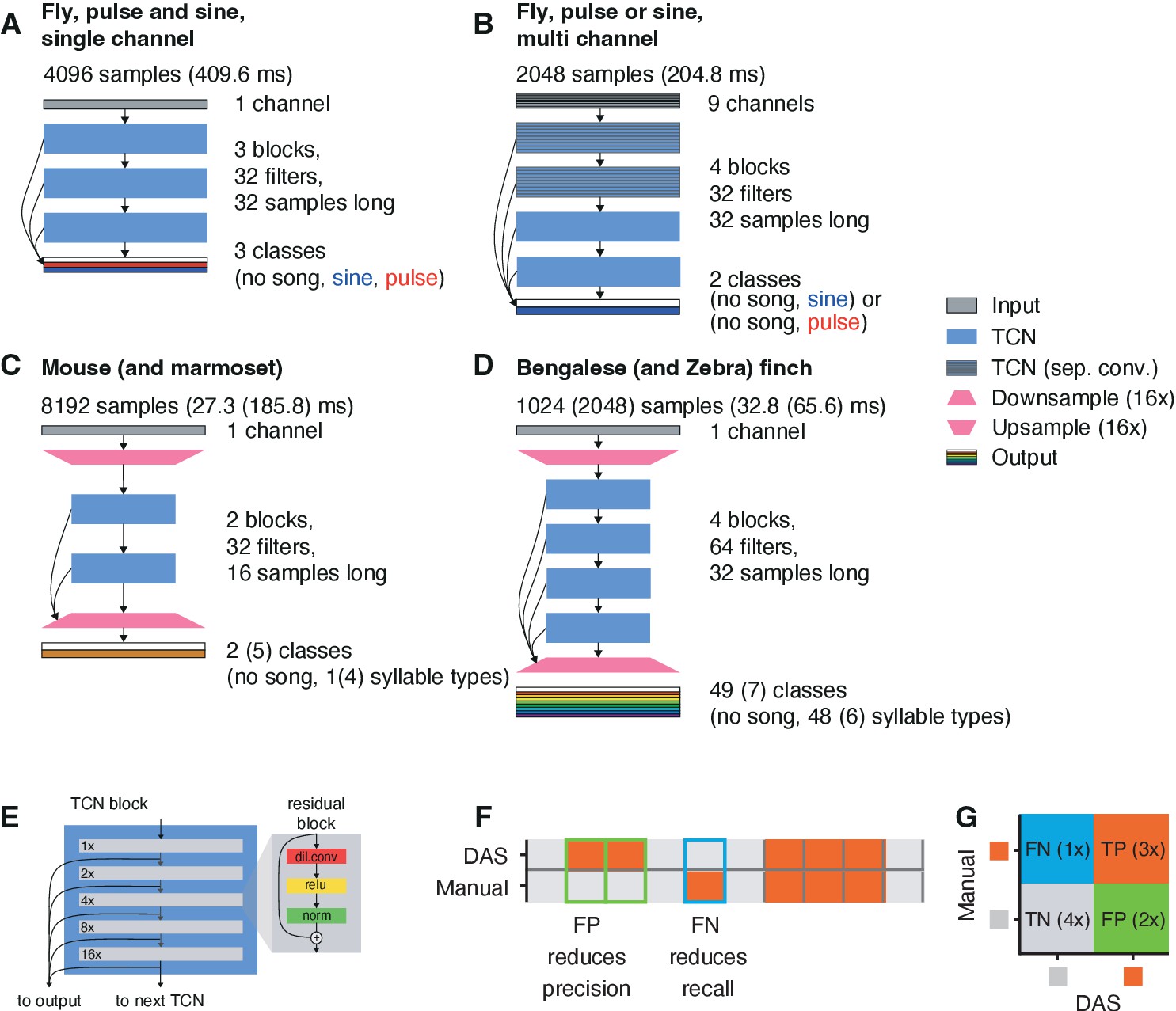
DAS architecture and evaluation.
(A-D) Network architectures for annotating fly song from single (A) and multi-channel (B) recordings, mouse USVs and marmoset song (C), and bird song (Bengalese and Zebra finches) (D). See legend to the right. Each TCN block consists of stacks of residual blocks shown in E. See Table 4 for all network parameters. (E) A TCN block (left) consists of a stack of five residual blocks (right). Residual blocks process the input with a sequence of dilated convolution, rectification (ReLU) and normalization. The output of this sequence of steps is then added to the input. In successive residual blocks, the dilation rate of the convolution filters doubles from 1x in the first to 16x in the last layer (see numbers to the left of each block). The output of the last residual block is passed as an input to the next TCN block in the network. In addition, the outputs of all residual blocks in a network are linearly combined to predict the song. (F) Annotation performance is evaluated by comparing manual annotations (top) with labels produced by DAS (bottom). Gray indicates no song, orange song. True negatives (TN) and true positives (TP) are samples for which DAS matches the manual labels. False negatives (FNs) are samples for which the song was missed (blue frame) and reduce recall (TP/(FN+TP)). False positives (FP) correspond to samples that were falsely predicted as containing song (green frames) and reduce precision (TP/(TP+FP)). (G) Precision and recall are calculated from a confusion matrix which tabulates TP (orange), TN (gray), FP (green), FN (blue). In the example, precision is 3/(3+2) and recall is 3/(1+3).
Figure 1—figure supplement 2
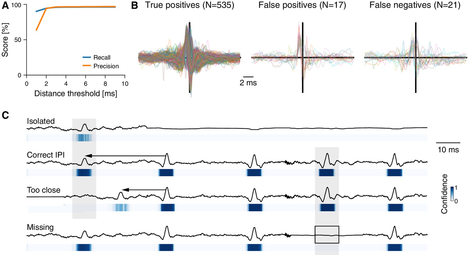
Performance and the role of context for annotating fly pulse song.
(A) Recall (blue) and precision (orange) for fly pulse song for different distance thresholds. The distance threshold determines the maximal distance to a true pulse for a detected pulse to be a true positive. (B) Waveforms of true positive (left), false positive (middle), and false negatives (right) pulses in fly song. Pulses were aligned to the peak, adjusted for sign, and their amplitude was normalized to have unit norm (see Clemens et al., 2018). (C) Waveforms (top) and confidence scores (bottom, see color bar) for pulses in different contexts. DAS exploits context effects to boost the detection of weak signals. An isolated ('Isolated', first row) weak pulse-like waveform is detected with low confidence, since similar waveforms often arise from noise. Manual annotators exploit context information—the fact that pulses often occur in trains at an interval of 40 ms—to annotate weak signals. DAS does the same: the same waveform is detected with much higher confidence due to the presence of a nearby pulse train ('Correct IPI', 2nd row). If the pulse is too close to another pulse ('Too close', 3rd row), it is likely noise and DAS detects it with lower confidence. Context effects do not affect strong signals. For instance, a missing pulse within a pulse train ('Missing', last row) does not reduce detection confidence of nearby pulses.
Figure 1—figure supplement 3
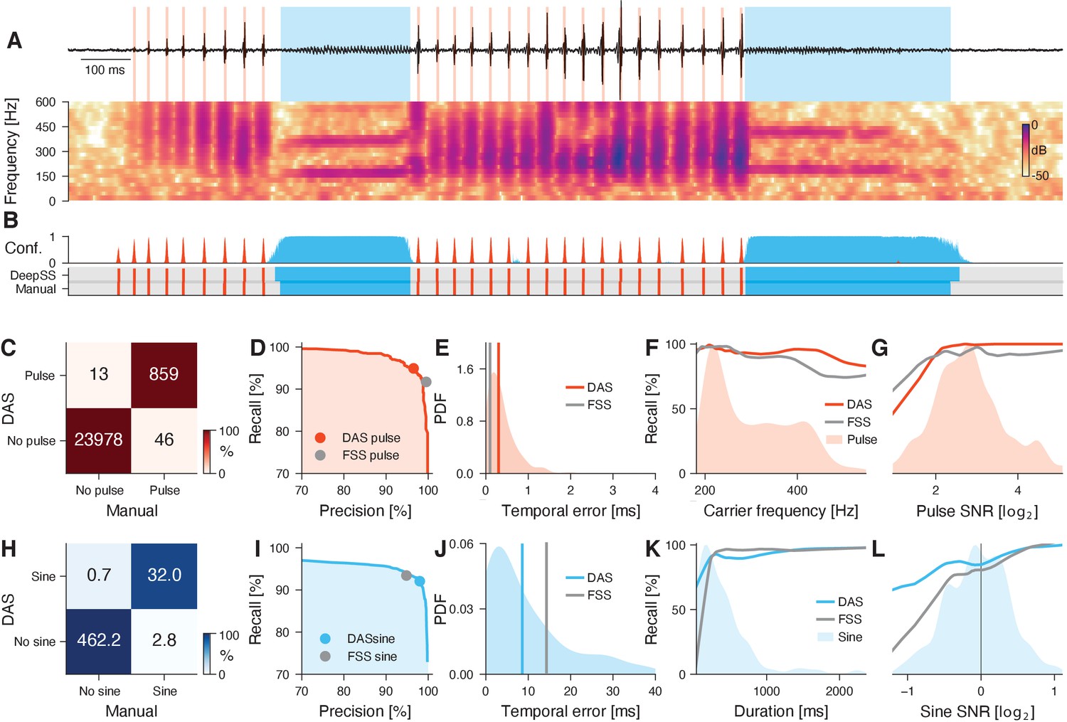
Performance for multi-channel recordings of fly courtship song.
(A) Fly song (black) with manual annotation indicating sine (blue) and pulse (red). Traces (top) and spectrogram (bottom, see color bar) show data from the loudest of the nine audio channels. (B) Confidence scores (top) for sine (blue) and pulse (red). The confidence is transformed into annotation labels (bottom) based on a confidence threshold (0.5 for sine and pulse). Ground truth (bottom) from manual annotations shown for comparison. DAS annotations were generated using separate networks for pulse and for sine. (C) Confusion matrix for pulse from a test data set. Color indicates the percentage (see color bar) and text labels indicate number of pulses for each quadrant. All confusion matrices are normalized such that columns sum to 100%. The concentration of values along the diagonal indicates high annotation performance. (D) Precision-recall curve for pulse depicts the performance characteristics of DAS for different confidence threshold (from 0 to 1). Recall decreases and precision increases with the threshold. The closer the curve to the upper and right border, the better. The red circle corresponds to the performance of DAS for a threshold of 0.5. The gray circle depicts the performance of FlySongSegmenter (FSS). (E) Probability density function (PDF) of temporal errors for all detected pulses (red shaded area), computed as the distance between each pulse annotated by DAS and its nearest manual pulse. Lines depict median temporal error for DAS (red line, 0.3 ms) and FSS (gray line, 0.1 ms). (F, G) Recall of DAS (red line) and FSS (gray line) as a function of the pulse carrier frequency (F) and signal-to-noise ratio (SNR) (G). Red areas show the distributions of carrier frequencies (F) and SNRs (G) for all pulses. (H) Same as in C but for sine. Color indicates the percentage (see color bar) and text labels indicate seconds of sine for each quadrant. (I) Same as in D but for sine. The blue circle depicts the performance for the confidence threshold of 0.5 used in A. (J) Distribution of temporal errors for all detected sine on- and offsets. Median temporal error is 9 ms for DAS (blue line) and 14 ms for FSS (gray line). (K, L) Recall for DAS (blue line) and FSS (gray line) as a function of sine duration (K) and SNR (L). Blue-shaded areas show the distributions of durations (K) and SNRs (L) for all sine songs. DAS outperforms FSS for sine songs with short durations and SNRs <1.0.
Figure 2 with 1 supplement
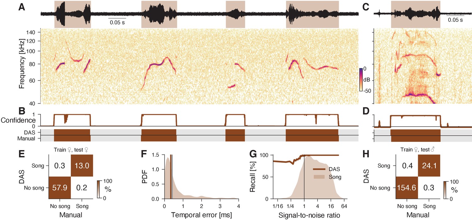
DAS performance for mouse ultrasonic vocalizations.
(A) Waveform (top) and spectrogram (bottom) of USVs produced by a female mouse in response to an anesthetized female intruder. Shaded areas (top) show manual annotations. (B) Confidence scores (top) and DAS and manual annotations (bottom) for the female USVs in A. Brief gaps in confidence are filled smooth annotations. (C) Example of male USVs with sex-specific characteristics produced in the same assay. (D) Confidence scores (top) and DAS and manual annotations (bottom) for the male USVs in C from a DAS network trained to detect female USVs. (E) Confusion matrix from a female-trained network for a test set of female USVs. Color indicates the percentage (see color bar) and text labels the seconds of song in each quadrant. (F) Distribution of temporal errors for syllable on- and offsets in female USVs. The median temporal error is 0.3 ms for DAS (brown line) and 0.4 ms for USVSEG Tachibana et al., 2020, a method developed to annotate mouse USVs (gray line). (G) Recall of the female-trained network (brown line) as a function of SNR. The brown shaded area represents the distribution of SNRs for all samples containing USVs. Recall is high even at low SNR. (H) Confusion matrix of the female-trained DAS network for a test set of male USVs (see C, D for examples). Color indicates the percentage (see color bar) and text labels the seconds of song in each quadrant.
Figure 2—figure supplement 1
Performance for marmoset vocalizations.
(A, C) Waveform (top) and spectrogram (bottom) of vocalizations from male and female marmosets. Shaded areas (top) show manual annotations of the different vocalization types, colored by type. Recordings are noisy (A, left), clipped (orange), and individual vocalization types are variable (C). (B, D) DAS and manual annotation labels for the vocalizations types in the recordings in A and C (see color bar in C). DAS annotates the syllable boundaries and types with high accuracy. Note the false negative in D. (E, F) Confusion matrices for the four vocalization types in the test set (see color bar), using the syllable boundaries from the manual annotations (E) or from DAS (F) as reference. Rows depict the probability with which DAS annotated each syllable as one of the four types in the test dataset. The type of most syllables were correctly annotated, resulting in the concentration of probability mass along the main diagonal. False positives and false negatives correspond to the first row in E and the first column in F, respectively. When using the true syllables for reference, there are no false positives (E, x=‘noise’, gray labels) since all detections are positives. By contrast, when using the predicted syllables as reference, there are no true negatives (F, y=‘noise’, gray labels), since all reference syllables are (true or false) positives. (G) Distribution of temporal errors for the on- and offsets of all detected syllables (purple-shaded area). The median temporal error is 4.4 ms for DAS (purple line) and 12.5 ms for the method by Oikarinen et al., 2019 developed to annotate marmoset calls (gray line).
Figure 3 with 2 supplements
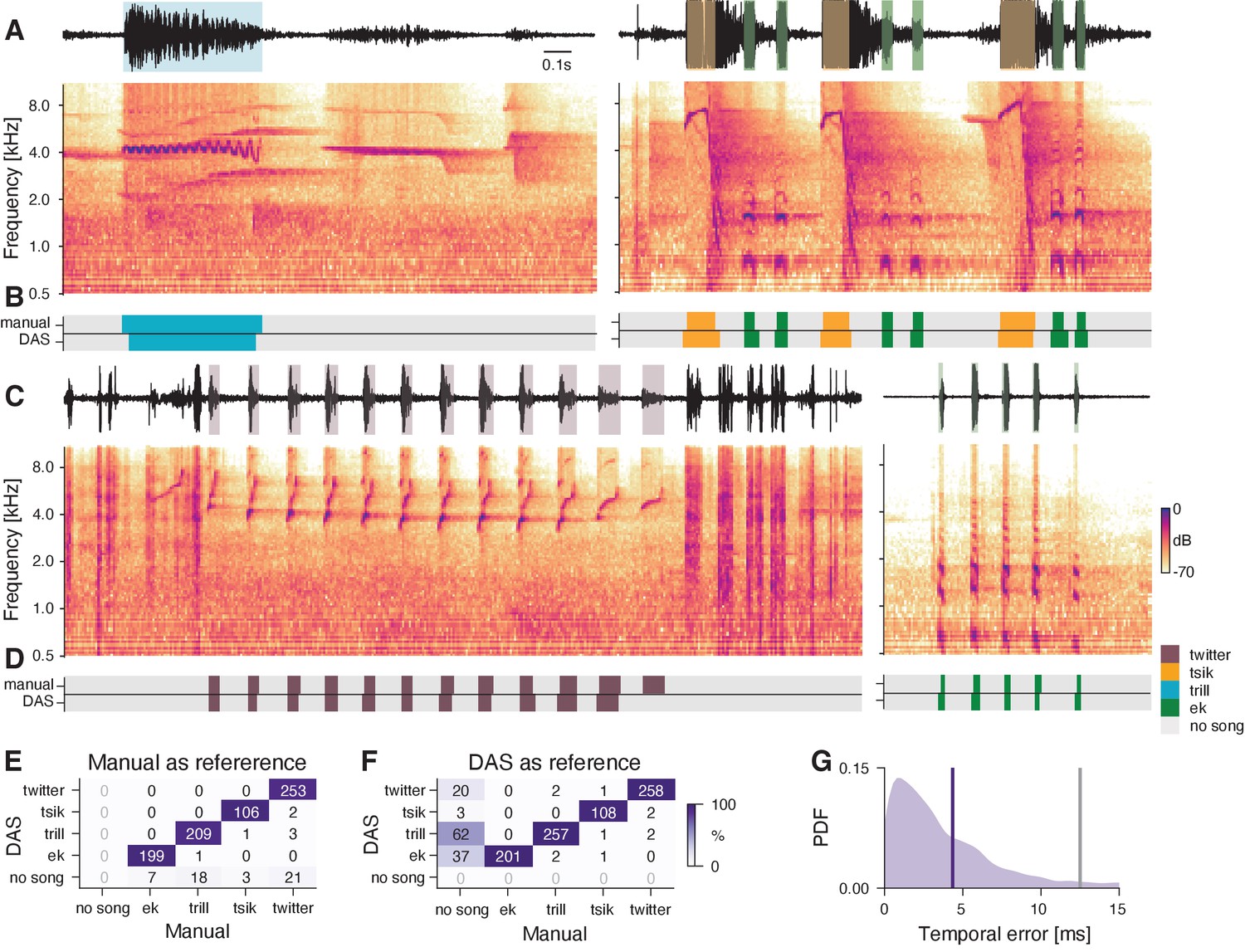
DAS performance for the song of Bengalese finches.
(A) Waveform (top) and spectrogram (bottom) of the song of a male Bengalese finch. Shaded areas (top) show manual annotations colored by syllable type. (B) DAS and manual annotation labels for the different syllable types in the recording in A (see color bar). DAS accurately annotates the syllable boundaries and types. (C) Confusion matrix for the different syllables in the test set. Color was log-scaled to make the rare annotation errors more apparent (see color bar). Rows depict the probability with which DAS annotated each syllable as any of the 37 types in the test dataset. The type of 98.5% of the syllables were correctly annotated, resulting in the concentration of probability mass along the main diagonal. (D) Distribution of temporal errors for the on- and offsets of all detected syllables (green-shaded area). The median temporal error is 0.3 ms for DAS (green line) and 1.1 ms for TweetyNet Cohen et al., 2020, a method developed to annotate bird song (gray line).
Figure 3—figure supplement 1
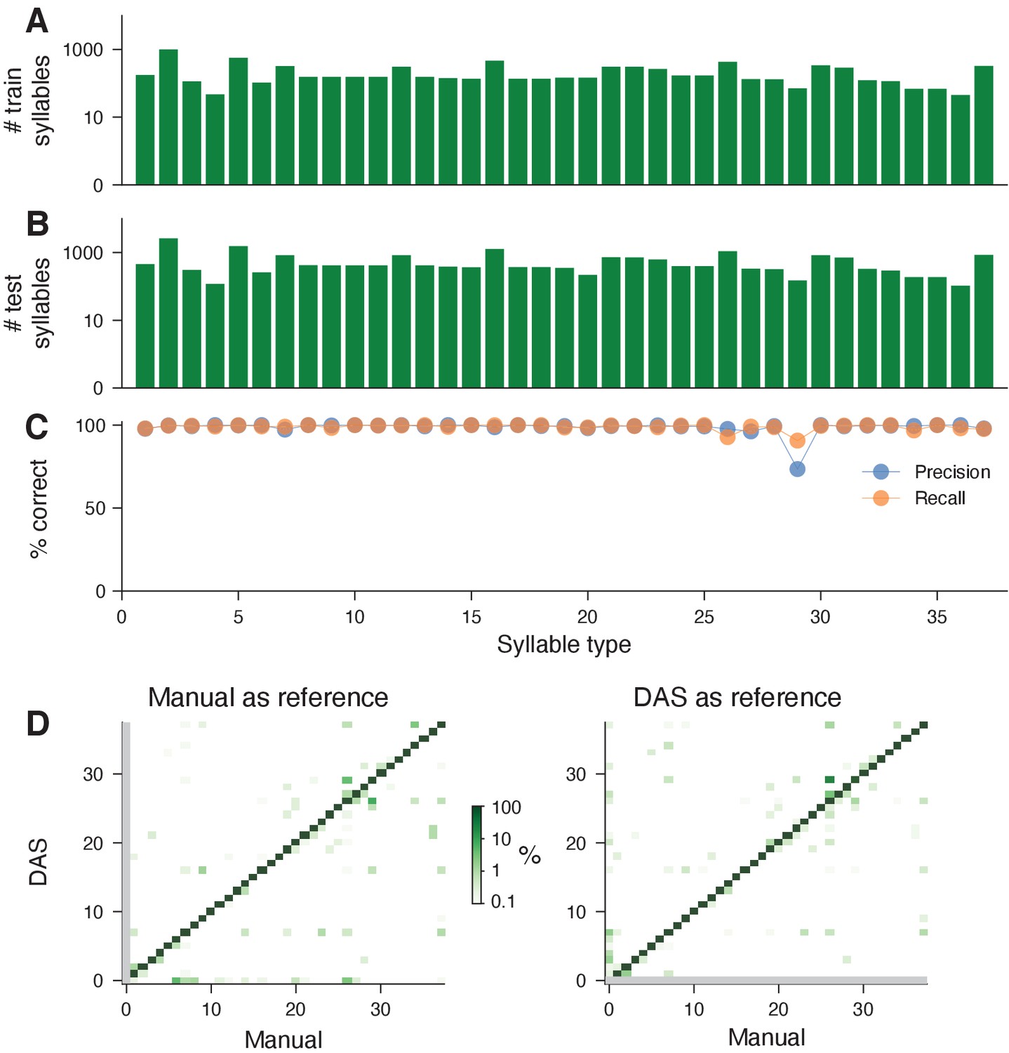
Performance for the song of Bengalese finches.
(A, B) Number of syllables (log scaled) in the train (A) and the test (B) sets for each syllable type present in the test set. (C) Precision (blue) and recall (orange) for each syllable type, computed from the confusion matrix in Figure 3C. (D) Confusion matrices when using true (left, same as Figure 3C) and predicted (right) syllables as a reference. Colors were log-scaled to make the rare annotation errors more apparent (see color bar). The reference determines the syllable bounds and the syllable label is then given by the most frequent label found in the samples within the syllable bounds. When using the true syllables for reference, there are no false positives (left, y=0 (no song), gray line) since all detections are positives. By contrast, when using the predicted syllables as reference, there are no true negatives (right, x=0 (no song), gray line), since all reference syllables are (true or false) positives. The average false negative and positive rates are 0.3% and 0.2%, respectively.
Figure 3—figure supplement 2
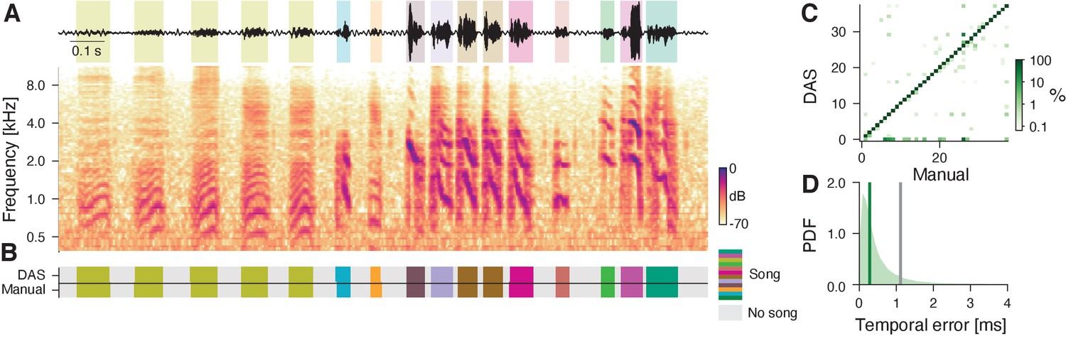
Performance for the song of a Zebra finch.
(A) Waveform (top) and spectrogram (bottom) of the song of a male Zebra finch. Shaded areas (top) show manual annotations of the six syllables of the male’s motif, colored by syllable type. (B) DAS and manual annotation labels for the six syllable types in the recording in A (see color bar). DAS accurately annotates the syllable boundaries and types. (C) Confusion matrix for the six syllables in the test set (see color bar). Rows depict the probability with which DAS annotated each syllable as any of the six types in the test dataset. The type of 100% (54/54) of the syllables were correctly annotated, resulting in the concentration of probability mass along the main diagonal. (D) Distribution of temporal errors for the on- and offsets of all detected syllables in the test set (blue-shaded area). The median temporal error is 1.3 ms for DAS (blue line) and 2 ms for TweetyNet (Cohen et al., 2020), a method developed to annotate bird song (gray line).
Figure 4 with 5 supplements

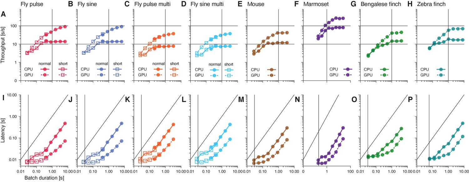
DAS annotates song with high throughput and low latency and requires little data.
(A, B) Throughput (A) and latency (B) of DAS (see also Figure 4—figure supplement 1). Throughput (A) was quantified as the amount of audio data in seconds annotated in one second of computation time. Horizontal lines in A indicate throughputs of 1, 10, 40, and 100. Throughput is >8x realtime on a CPU (dark shades) and >24x or more on a GPU (light shades). Latency (B) corresponds to the time it takes to annotate a single chunk of audio and is similar on a CPU (dark shades) and a GPU (light shades). Multi-channel audio from flies was processed using separate networks for pulse and sine. For estimating latency of fly song annotations, we used networks with 25 ms chunks, not the 410 ms chunks used in the original network (see Figure 1—figure supplement 2). (C) Flow diagram of the iterative protocol for fast training DAS. (D) Number of manual annotations required to reach 90% of the performance of DAS trained on the full data set shown in Figure 1, Figure 1—figure supplement 3, Figure 2, Figure 2—figure supplement 1, Figure 3, and Figure 3—figure supplement 2 (see also Figure 4—figure supplement 3). Performance was calculated as the F1 score, the geometric mean of precision and recall. For most tasks, DAS requires small to modest amounts of manual annotations. (E) Current best validation loss during training for fly pulse song recorded on a single channel for 10 different training runs (red lines, 18 min of training data). The network robustly converges to solutions with low loss after fewer than 15 min of training (40 epochs).
Figure 4—figure supplement 1
Throughput and latency of inference.
Median throughput (A–H) and latency (I–P) across 10 inference runs for different song types. Batch duration is the product of chunk duration and batch size. Error bars are smaller than the marker size (see Figure 4A/B). Solid and dashed lines correspond to values when running DAS on a CPU and GPU, respectively. Squares and circles in the plots for fly song correspond to networks with short and long chunk durations, respectively (see Figure 4—figure supplement 2). In A-H, horizontal lines mark 10x and 100x realtime and vertical lines mark the batch duration used in Figure 4A. In I-P, the vertical line marks the batch duration used in Figure 4B. Differences in the throughput and latency between species arise from differences in the sample rate and the complexity of the network (number and duration of the filters, number of TCN blocks) (see Table 4).
Figure 4—figure supplement 2
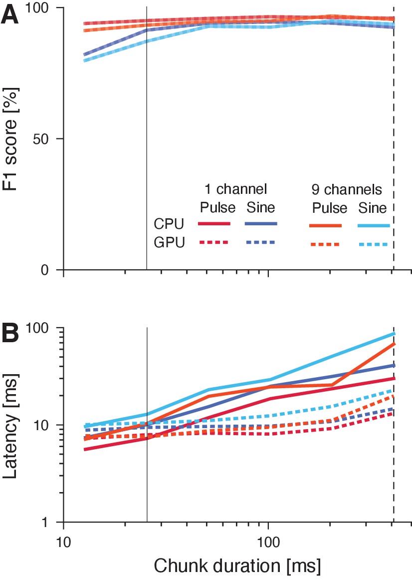
Reducing the chunk duration reduces latency and comes with minimal performance penalties.
(A) F1 scores of networks with different chunk durations. Reduction of performance due to loss of context information with shorter chunks is minimal. (B) Latency of networks with different chunk durations. Dashed vertical lines indicate the chunk durations of the networks in Figure 1, Figure 4B and Figure 4—figure supplement 1. Solid vertical lines indicated the ‘short’ chunk durations used in Figure 4B and Figure 4—figure supplement 1.
Figure 4—figure supplement 3
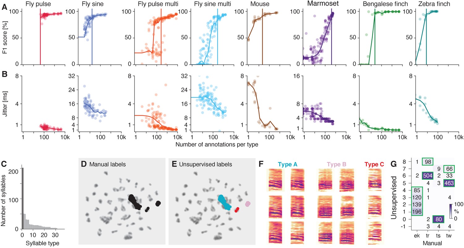
DAS requires small to moderate amounts of data for training.
(A) Performance as a function of the number of manual annotations in the training set. Individual dots correspond to individual fits using different subsets of the data. For flies and mice, dots indicate the number of annotations for each type and performance is given by the F1 score—the geometric mean of precision and recall. For the marmosets and birds (rightmost panels), dots correspond to the median number of syllables per type in the training set and performance is given by the median accuracy over syllables per fit (see C for per-type statistics for Bengalese finches). Colored curves in A and B were obtained by locally weighted scatter plot smoothing (lowess) of the individual data points. Vertical lines correspond to the number of syllables required to surpass 90% of the maximal performance. (B) Temporal error given as the median temporal distance to syllable on- and offsets or to pulses. (C) Number of annotations required per syllable type for Bengalese finches (range 2–64, median 8, mean 17). One outlier type requires 200 annotations and consists of a mixture of different syllable types (black bar, see D-F). (D, E) UMAP embedding of the bird syllables with the outlier type from C labeled according to the manual annotations (D, black) and the unsupervised clustering (F). The unsupervised clustering reveals that the outlier type splits into two distinct clusters of syllables (cyan and pink) and three mislabeled syllables (red). (F) Spectrograms of different types of syllable exemplars from the outlier type in C grouped based on the unsupervised clustering in E. (G) Confusion matrix mapping manual to unsupervised cluster labels (see Figure 5F,G) for marmosets. Green boxes mark the most likely call type for each unsupervised cluster. While there is a good correspondence between manual and unsupervised call types, most call types are split into multiple clusters.
Figure 4—figure supplement 4
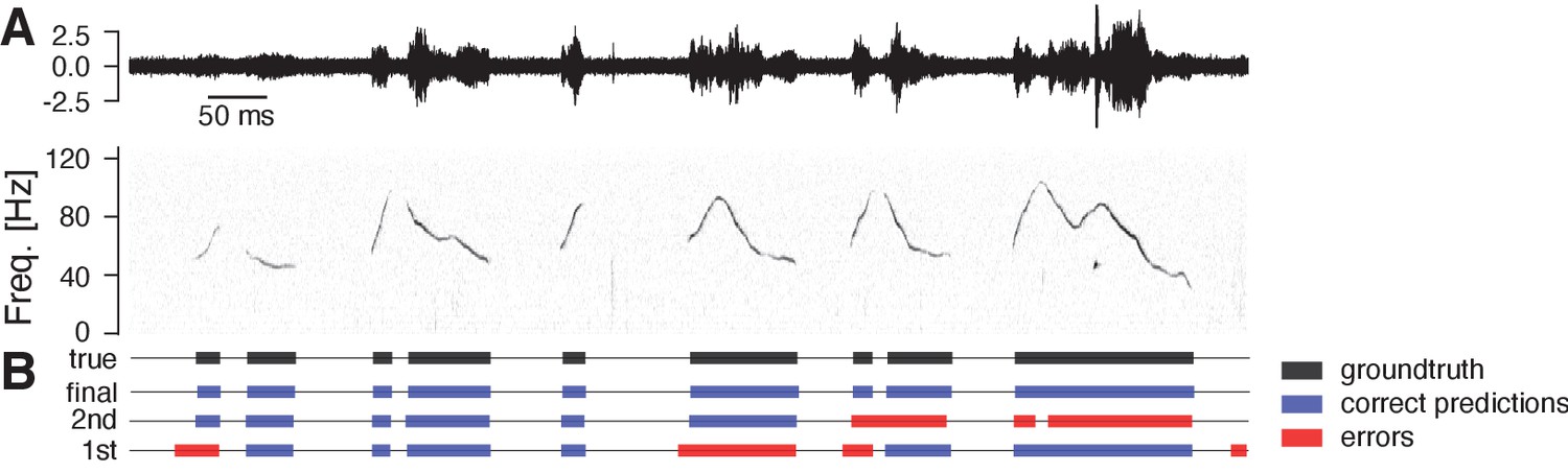
Example of fast training mouse USVs.
DAS can be trained using an iterative procedure, in which the network is trained after annotating few syllables. This initial network is then used to create a larger dataset of annotations, by predicting and manually correcting annotation labels for a longer stretch of audio. This procedure is repeated to create ever larger training datasets until the performance is satisfactory. Shown is an example from mouse USVs. (A) Example of the test recording for mouse USVs (top - waveform, bottom - spectrogram) (B) Manual labels (true, black) and correct (blue) and erroneous (red) annotations from DAS for three different stages of training. Even for the first round of fast training, the majority of onsets is detected with low temporal error, requiring only few corrections. Number of syllables, seconds of song and F1-score for the different iterations (1st/2nd/final): 72/248/2706 syllables, 6/26/433 s of song, F1 score 96.6/97.9/98.9%.
Figure 4—figure supplement 5
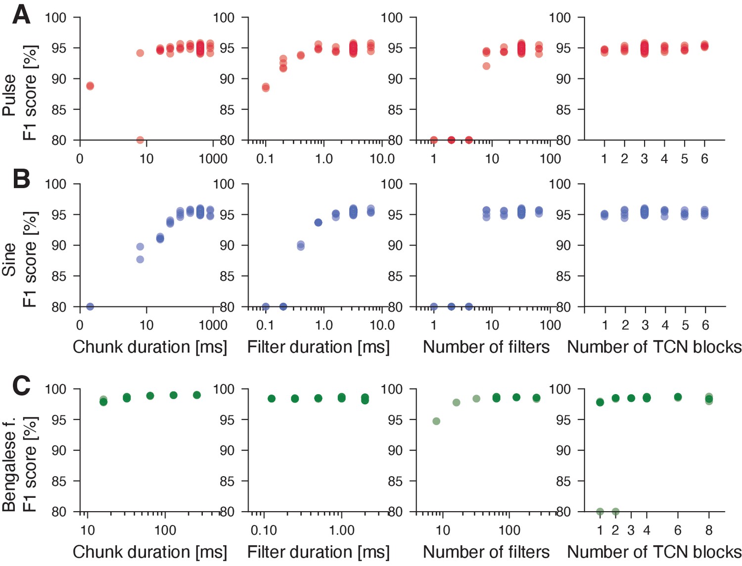
DAS performance is robust to changes in the structural parameters of the network.
(A, B) Performance (F1 score) for networks with different structural parameters for fly pulse (A, red) and sine (B, blue). The starting point for each modified network was the network given in Table 4. We then trained networks with modified structural parameters from scratch. As long as the network has chunks longer than 100 ms, filters longer than 2 ms, more than eight filters, and at least one TCN block, the resulting model has an F1 score of 95% for pulse and sine. (C) Same in in B but for Bengalese finches. Network performance is robust to changes in structural parameters. Convergence is inconsistent for shallow networks with 1–2 TCN blocks (rightmost panel). F1 scores smaller than 80% in A-C where set to 80% to highlight small changes in performance.
Figure 5
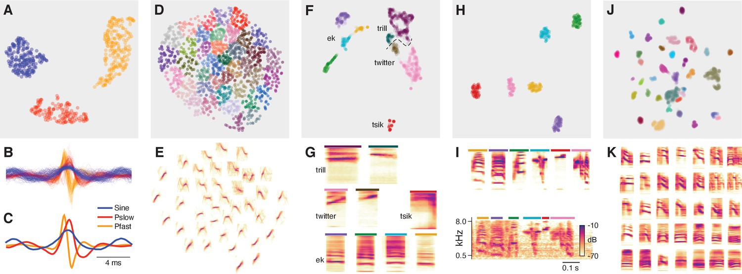
DAS can be combined with unsupervised methods for song classification.
(A) Low-dimensional representation obtained using the UMAP (McInnes and Healy, 2018) method of all pulse and sine song waveforms from Drosophila melanogaster annotated by DAS in a test data set. Data points correspond to individual waveforms and were clustered into three distinct types (colors) using the density-based method HDBSCAN (McInnes et al., 2017). (B, C) All waveforms (B) and cluster centroids (C) from A colored by the cluster assignment. Waveforms cluster into one sine (blue) and two pulse types with symmetrical (red, ) and asymmetrical (orange, ) shapes. (D, E) Low-dimensional representation of the spectrograms of mouse USVs (D) and mean spectrogram for each cluster in D (E). Individual syllables (points) form a continuous space without distinct clusters. Song parameters vary continuously within this space, and syllables can be grouped by the similarity of their spectral contours using k-means clustering. (F, G) Low-dimensional representation of the spectrograms of the calls from marmosets (F) and mean spectrogram for each cluster in F (G). Calls separate into distinct types and density-based clustering (colors) produces a classification of syllables that recovers the manual annotations (Figure 4—figure supplement 3G, homogeneity score 0.88, completeness score 0.57, v-score 0.69). Most types split into multiple clusters, reflecting the variability of the call types in marmosets. Colored bars on top of each spectrogram in G correspond to the colors for the individual clusters in F. The dashed line shows the boundary separating trills and twitters. (H, I) Low-dimensional representation of the spectrograms of the syllables from one Zebra finch male, mean spectrogram for each cluster in H (I, top), and example of each clustered syllable within the motif (I, bottom). Density-based clustering (colors) recovers the six syllable types forming the male’s motif. Colored bars on top of each spectrogram in I correspond to the colors for the individual clusters in H. (J, K) Low-dimensional representation of the spectrograms of the syllables from four Bengalese finch males (J) and mean spectrogram for each cluster in J (K). Syllables separate into distinct types and density-based clustering (colors) produces a classification of syllables that closely matches the manual annotations (homogeneity score 0.96, completeness score 0.89, v-score 0.92). X-axes of the average spectrograms for each cluster do not correspond to linear time, since the spectrograms of individual syllables were temporally log-rescaled and padded prior to clustering. This was done to reduce the impact of differences in duration between syllables.
Tables
Table 1
Comparison to human annotators for fly song.
See also Figure 1E,J.
| Annotator | Sine recall [%] | Sine precision [%] | Pulse recall [%] | Pulse precision [%] |
|---|---|---|---|---|
| Human A | 89 | 98 | 99 | 93 |
| Human B | 93 | 91 | 98 | 88 |
| FSS | 91 | 91 | 87 | 99 |
| DAS | 98 | 92 | 96 | 97 |
Table 2
Precision, recall, and temporal error of DAS.
Precision and recall values are sample-wise for all except fly pulse song, for which it is event-wise. The number of classes includes the ‘no song’ class. (p) Pulse, (s) Sine.
| Species | Trained | Classes | Threshold | Precision [%] | Recall [%] | Temporal error [ms] |
|---|---|---|---|---|---|---|
| Fly single channel | Pulse (p) and sine (s) | 3 | 0.7 | 97/92 (p/s) | 96/98 (p/s) | 0.3/12 (p/s) |
| Fly multi channel | Pulse (p) | 2 | 0.5 | 98 | 94 | 0.3 |
| Fly multi channel | Sine (s) | 2 | 0.5 | 97 | 93 | 8 |
| Mouse | Female | 2 | 0.5 | 98 | 99 | 0.3 |
| Marmoset | five male-female pairs | 5 | 0.5 | 85 | 91 | 4.4 |
| Bengalese finch | four males | 49 (38 in test set) | 0.5 | 97 | 97 | 0.3 |
| Zebra finch | one males | 7 | 0.5 | 98 | 97 | 1.2 |
Table 3
Comparison to alternative methods.
Methods used for comparisons: (1) Arthur et al., 2013, (2) Tachibana et al., 2020, (3) Oikarinen et al., 2019, (4) Cohen et al., 2020. (A,B) DAS was trained on 1825/15970 syllables which contained 4/7 of the call types from Oikarinen et al., 2019. (B) The method by Oikarinen et al., 2019 produces an annotation every 50 ms of the recording - since the on/offset can occur anywhere within the 50 ms, the expected error of the method by Oikarinen et al., 2019 is at least 12.5 ms. (C) The method by Oikarinen et al., 2019 annotates 60 minutes of recordings in 8 minutes. (D) Throughput assessed on the CPU, since the methods by Arthur et al., 2013 and Tachibana et al., 2020 do not run on a GPU. (E) Throughput assessed on the GPU. The methods by Cohen et al., 2020 and Oikarinen et al., 2019 use a GPU.
| Precision [%] | Recall [%] | Jitter [ms] | Throughput [s/s] | |||||
|---|---|---|---|---|---|---|---|---|
| Species | DAS | Other | DAS | Other | DAS | Other | DAS | Other |
| Fly single (1) | 97/92 (p/s) | 99/91 | 96/98 (p/s) | 87/91 | 0.3/12 (p/s) | 0.1/22 | 15 | 4 (D) |
| Fly multi (1) | 98 | 99 | 94 | 92 | 0.3 | 0.1 | 8 (p) | 0.4 (p+s) (D) |
| Fly multi (1) | 97 | 95 | 93 | 93 | 8.0 | 15.0 | 8 (s) | 0.4 (p+s) (D) |
| Mouse (2) | 98 | 98 | 99 | 99 | 0.3 | 0.4 | 12 | 4 (D) |
| Marmoset (3) | 96 | 85 (A) | 92 | 77 (A) | 4.4 | 12.5 (B) | 82 | 7.5 (C, E) |
| Bengalese finch (4) | 99 | 99 | 99 | 99 | 0.3 | 1.1 | 15 | 5 (E) |
| Zebra finch (4) | 100 | 100 | 100 | 100 | 1.3 | 2.0 | 18 | 5 (E) |
Table 4
Structural parameters of the tested networks.
| Species | Rate [kHz] | Chunk [samples] | Channels | STFT downsample | Separable conv. | TCN stacks | Kernel size [samples] | Kernel |
|---|---|---|---|---|---|---|---|---|
| Fly single channel | 10.0 | 4096 | 1 | - | - | 3 | 32 | 32 |
| Fly multi channel (pulse) | 10.0 | 2048 | 9 | - | TCN blocks 1+2 | 4 | 32 | 32 |
| Fly multi channel (sine) | 10.0 | 2048 | 9 | - | TCN blocks 1+2 | 4 | 32 | 32 |
| Mouse | 300.0 | 8192 | 1 | 16x | - | 2 | 16 | 32 |
| Marmoset | 44.1 | 8192 | 1 | 16x | - | 2 | 16 | 32 |
| Bengales finch | 32.0 | 1024 | 1 | 16x | - | 4 | 32 | 64 |
| Zebra finch | 32.0 | 2048 | 1 | 16x | - | 4 | 32 | 64 |
Table 5
Sources of all data used for testing DAS.
‘Data’ refers to the data used for DAS and to annotations that were either created from scratch or modified from the original annotations (deposited under https://data.goettingen-research-online.de/dataverse/das). ‘Original data’ refers to the recordings and annotations deposited by the authors of the original publication. ‘Model’ points to a directory with the model files as well as a small test data set and demo code for running the model (deposited under https://github.com/janclemenslab/das-menagerie).
Additional files
Download links
A two-part list of links to download the article, or parts of the article, in various formats.
Downloads (link to download the article as PDF)
Open citations (links to open the citations from this article in various online reference manager services)
Cite this article (links to download the citations from this article in formats compatible with various reference manager tools)
Fast and accurate annotation of acoustic signals with deep neural networks
eLife 10:e68837.
https://doi.org/10.7554/eLife.68837


