Decoding the brain state-dependent relationship between pupil dynamics and resting state fMRI signal fluctuation
- Translational Neuroimaging and Neural Control Group, High Field Magnetic Resonance Department, Max Planck Institute for Biological Cybernetics, Germany
- Graduate Training Centre of Neuroscience, International Max Planck Research School, University of Tuebingen, Germany
- Institute of Neuroscience and Medicine 4, Medical Imaging Physics, Forschungszentrum Jülich, Germany
- Athinoula A. Martinos Center for Biomedical Imaging, Massachusetts General Hospital and Harvard Medical School, United States
Figures
Figure 1

Variability of the pupil–fMRI linkage.
(A) Pupil–fMRI correlation map created by correlating the two modalities’ concatenated signals from all trials. (B) Selected individual-trial correlations maps. (C) Histogram of spatial correlations between the all-trial correlation map and individual-trial maps. High variability of similarities between the maps shows that the pupil–fMRI relationship is not stationary and changes across trials.
-
Figure 1—source data 1
The mean correlation map (A), all individual correlation maps (B), and the spatial correlation values (C) are available in the source data file.
- https://cdn.elifesciences.org/articles/68980/elife-68980-fig1-data1-v2.zip
Figure 2 with 6 supplements
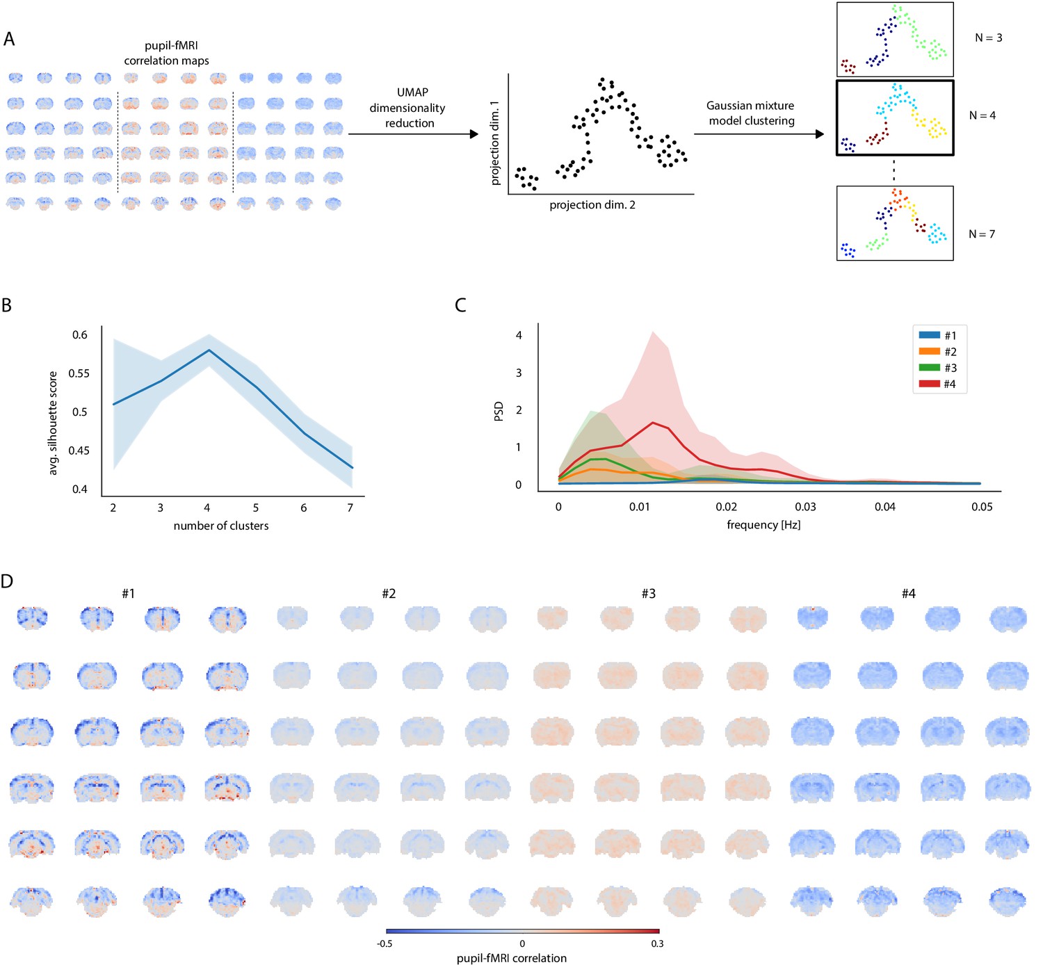
Clustering of trials with distinct pupil–fMRI correlation patterns.
(A) Schematic of the clustering procedure. UMAP is used to reduce the dimensionality of all individual-trial correlation maps to 72 dimensions. A 2D UMAP-projection of the real data is shown. Each dot represents a single trial. The trials are clustered using Gaussian mixture model clustering. Different numbers of clusters are evaluated. (B) The final number of clusters is selected based on silhouette analysis. The highest average silhouette score is obtained with k = 4 clusters. Shaded area shows standard deviations. (C) Pupil power spectral density estimates (PSD) of each of the four clusters. Signals were downsampled to match the fMRI sampling rate. Shaded areas show standard deviations. (D) Cluster-specific correlation maps based on concatenated signals belonging to the respective groups.
-
Figure 2—source data 1
Cluster trial labels, individual silhouette scores (B), mean cluster PSDs (C), and cluster-specific correlation maps (D) are available in the source data file.
- https://cdn.elifesciences.org/articles/68980/elife-68980-fig2-data1-v2.zip
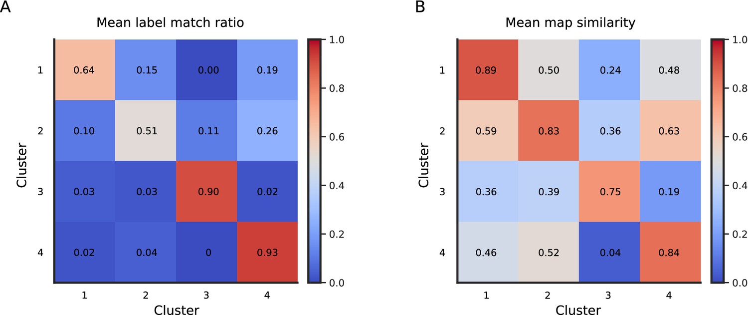
Figure 2—figure supplement 1
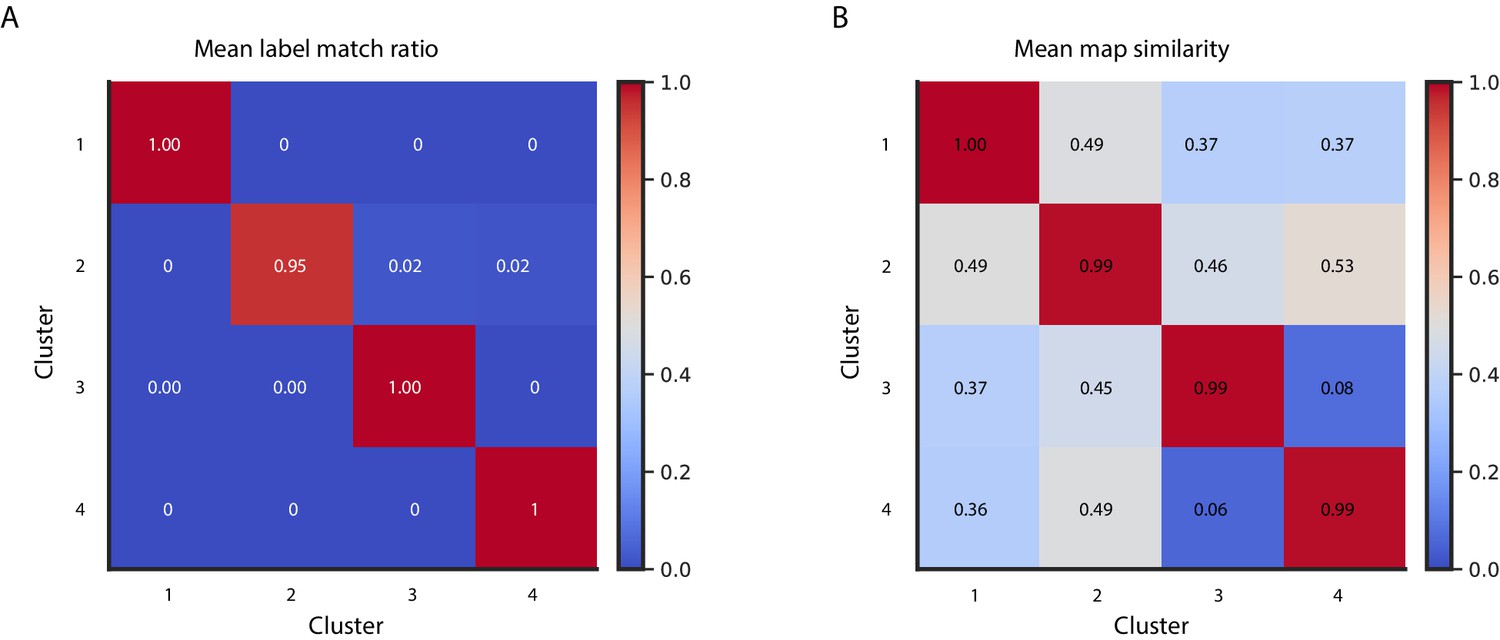
Cluster reproducibility across 100 repetitions with random UMAP and GMM initializations.
(A) Matrix displaying the ratio of cluster membership labels matching the most common cluster membership assignment across the 100 repetitions. (B) Matrix displaying the mean spatial correlation between the 100 cluster-specific maps and the maps based on the most common cluster membership assignment.
-
Figure 2—figure supplement 1—source data 1
The label match ratios (A) and map similarity values (B) are available in the source data file.
- https://cdn.elifesciences.org/articles/68980/elife-68980-fig2-figsupp1-data1-v2.zip
Figure 2—figure supplement 2
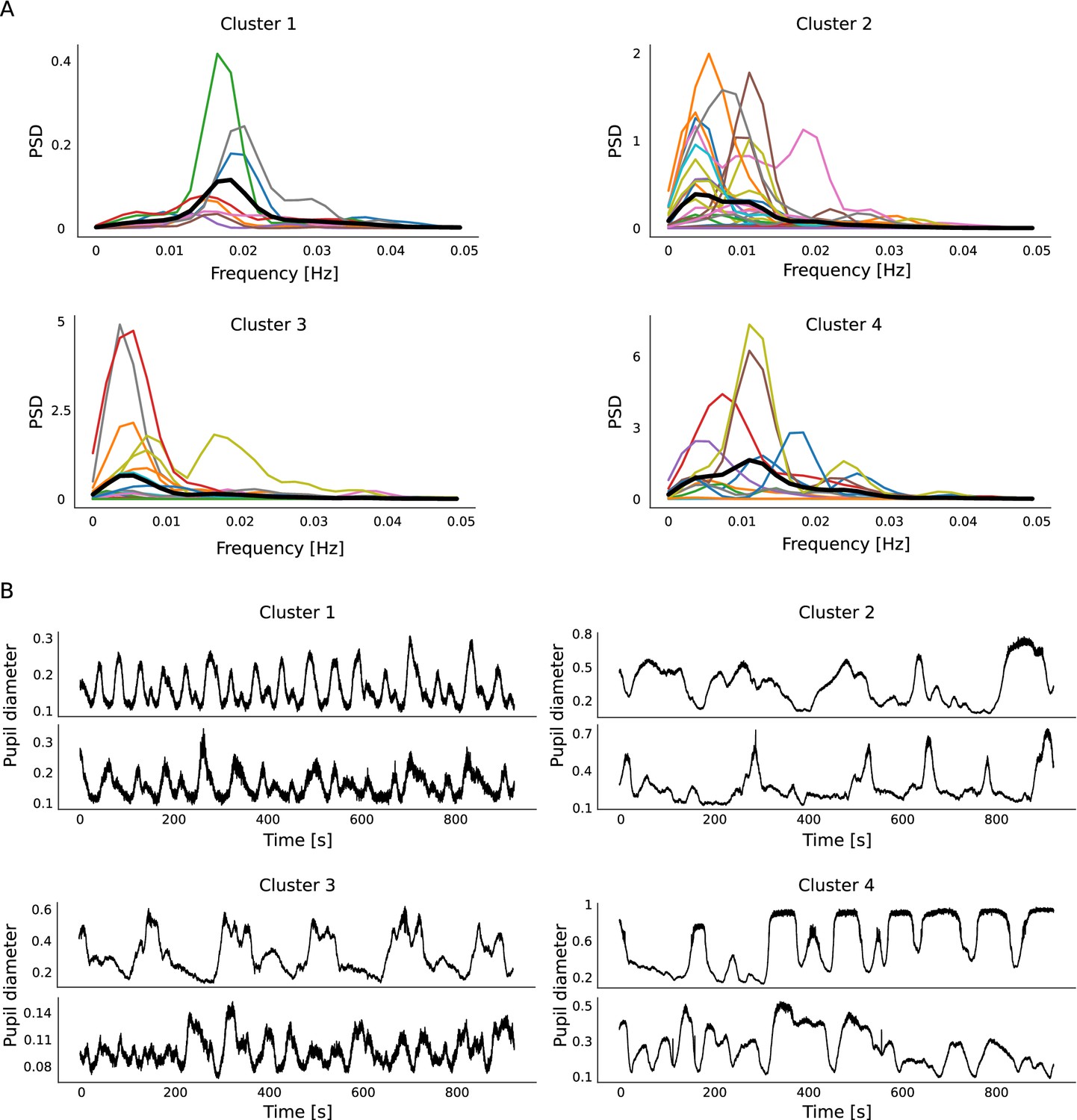
Cluster-specific pupil fluctuation features.
(A) PSDs of all trials divided based on their cluster memberships. Clusters 1 and 3 show specific peak frequencies. Cluster 4 shows the largest PSDs, hence the largest pupil size fluctuations. Cluster 1 shows the opposite. (B) Two example pupil diameter time courses are plotted per cluster. The magnitude of changes reflects the PSD differences visible in (A).
-
Figure 2—figure supplement 2—source data 1
All PSDs (A) are available in the source data file.
All pupil signals (B) are available online (see Materials and methods).
- https://cdn.elifesciences.org/articles/68980/elife-68980-fig2-figsupp2-data1-v2.zip
Figure 2—figure supplement 3
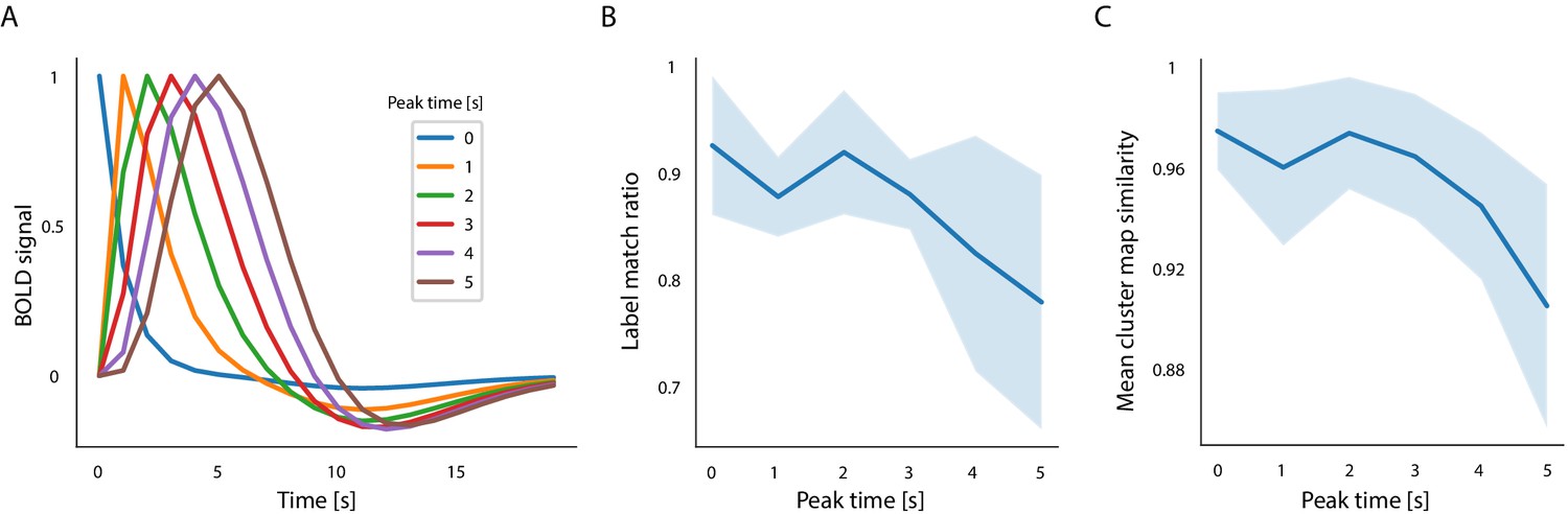
Clustering reproducibility across 100 clustering repetitions based on HRF-convolved pupil signals.
(A) HRFs with different peak times were used to create the convolved and lagged pupil signals. (B) Mean match ratio of cluster membership labels created using the convolved signals and those employed throughout the manuscript. The shaded area shows the standard deviation. (C) Mean spatial correlation between cluster-specific maps created using the convolved and non-convolved signals. The shaded area shows the standard deviation.
-
Figure 2—figure supplement 3—source data 1
The HRF kernels (A), cluster membership label match ratios (B), and map similarity values (C) are available in the source data file.
- https://cdn.elifesciences.org/articles/68980/elife-68980-fig2-figsupp3-data1-v2.zip
Figure 2—figure supplement 4
Cluster reproducibility across 100 repetitions of split-halves clustering.
(A) Matrix displaying the ratio of split-halves cluster membership labels matching the cluster membership assignment based on all trials across 100 repetitions. (B) Matrix displaying the mean spatial correlation between the 100 split-halves cluster-specific maps and maps based on all trials.
-
Figure 2—figure supplement 4—source data 1
The label match ratios (A) and map similarity values (B) are available in the source data file.
- https://cdn.elifesciences.org/articles/68980/elife-68980-fig2-figsupp4-data1-v2.zip
Figure 2—figure supplement 5
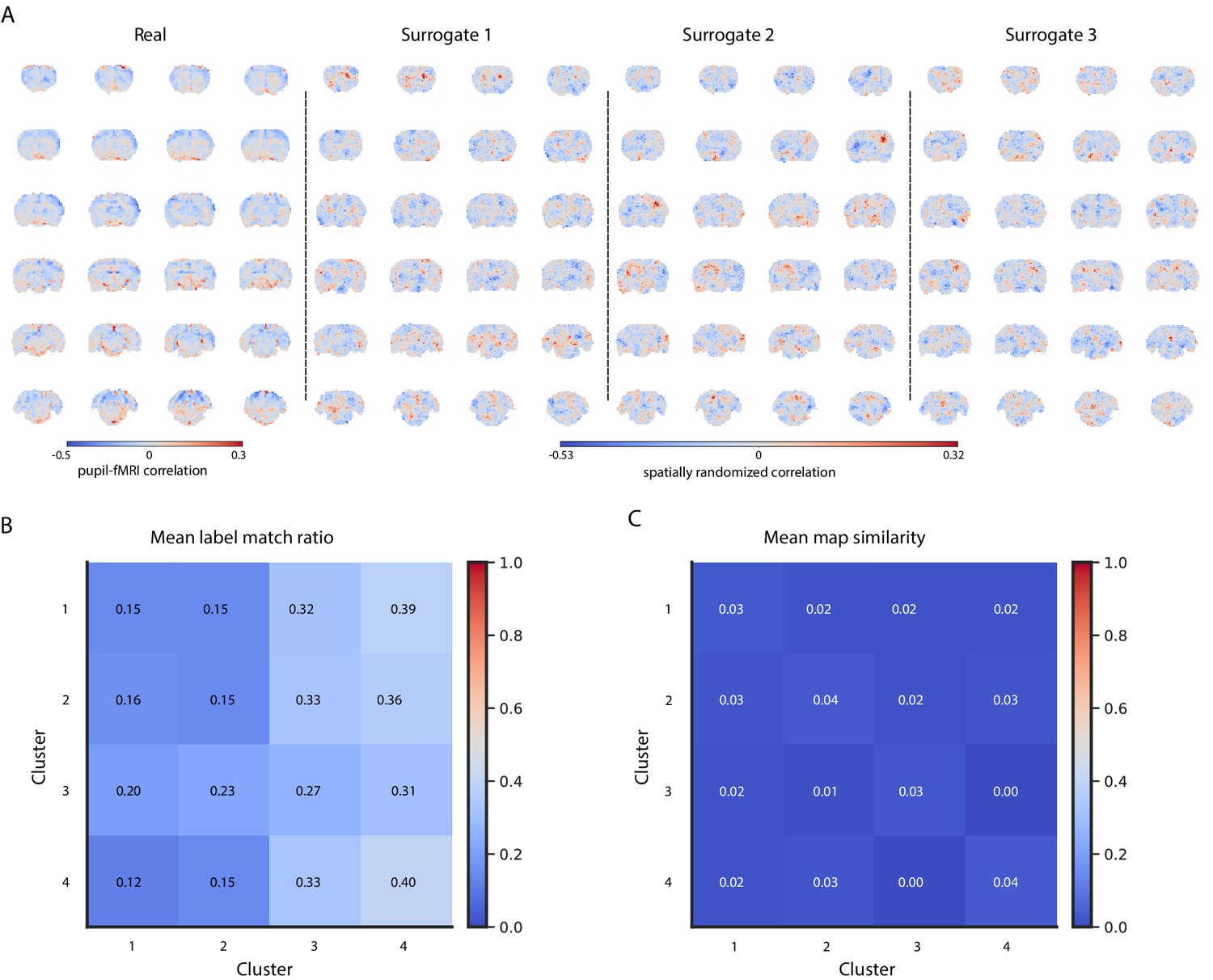
Cluster reproducibility across 100 sets of artificially generated surrogates with values and spatial autocorrelations matching those of real maps.
(A) A real pupil–fMRI correlation map and three example surrogate maps. (B) Matrix displaying the ratio of cluster membership labels generated based on the surrogate maps and those based on real data. (C) Matrix displaying the mean spatial correlation between the surrogate cluster-specific maps and those based on real data.
-
Figure 2—figure supplement 5—source data 1
Ten example surrogate sets (i.e. 740 maps total) (A), label match ratios (B), and map similarity values (C) are available in the source data file.
- https://cdn.elifesciences.org/articles/68980/elife-68980-fig2-figsupp5-data1-v2.zip
Figure 2—figure supplement 6
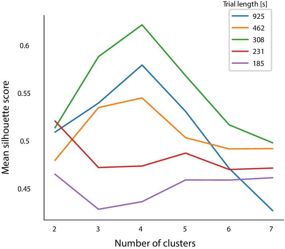
Mean silhouette scores based on 100 clustering repetitions performed on shorter trials.
Based on the silhouette score criterion, the n = 4 clusters result should be chosen even when dividing the trials into three parts.
-
Figure 2—figure supplement 6—source data 1
Individual silhouette scores are available in the source data file.
- https://cdn.elifesciences.org/articles/68980/elife-68980-fig2-figsupp6-data1-v2.zip
Figure 3 with 3 supplements
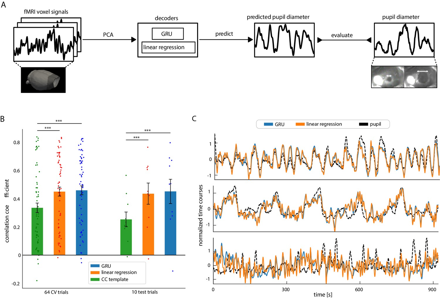
Decoding pupil dynamics based on fMRI signals.
(A) Schematic of the decoding procedure. PCA was applied to fMRI data. The PCA time courses were fed into either linear regression or GRU decoders, which generated pupil signal predictions. The prediction quality was evaluated by comparing the generated signals with real pupil fluctuations using Pearson’s correlation coefficients. (B) Comparison of the three methods’ pupil dynamics predictions. Linear regression and GRU performed better than the correlation-based baseline method on both the cross-validation splits (CCbase = 0.37 ± 0.27 s.d., CCLR = 0.45 ± 0.26 s.d., CCGRU = 0.46 ± 0.25 s.d., pLR = 4.3*10–6, pGRU = 2.4 × 10⁻⁶) and on test data (CCbase = 0.25 ± 0.17 s.d., CCLR = 0.44 ± 0.24 s.d., CCGRU = 0.45 ± 0.27 s.d., pLR = 0.003, pGRU = 0.01). Scattered points show individual prediction scores. (C) Linear regression and GRU predictions of three selected trials (CCGRU-top = 0.79, CCLR-top = 0.77, CCGRU-middle = 0.75,CCLR-middle = 0.73, CCGRU-bottom = 0.02, CCLR-bottom = 0.06). Qualitatively, linear regression and GRU predictions were very similar.
-
Figure 3—source data 1
Prediction scores (B) and all predicted time courses (C) are available in the source data file.
- https://cdn.elifesciences.org/articles/68980/elife-68980-fig3-data1-v2.zip
Figure 3—figure supplement 1
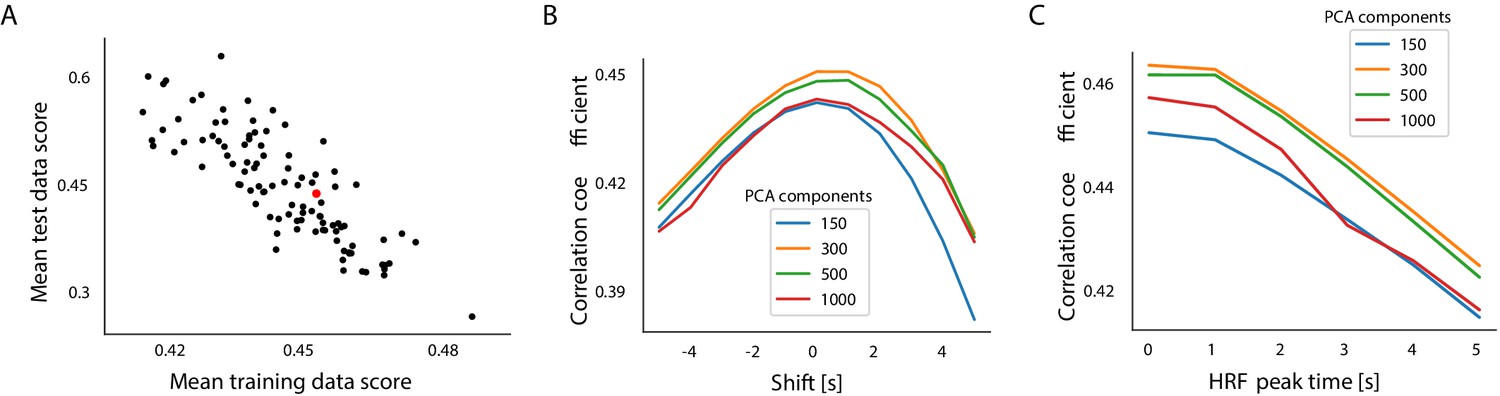
Prediction score dependence on train-test split trial selection, number of PCA components, and temporal shifts between pupil and fMRI signals.
(A) Mean test and train set prediction scores across 100 random train-test splits. The red dot shows values described in the manuscript. (B) The influence of temporal shifts and different component counts on prediction scores. Temporally shifting the fMRI and pupil fluctuation signals reduced prediction accuracy. Predictions generated based on 300 PCA components obtained the best scores. (C) The influence of predicting the HRF-convolved pupil signals and using different component counts on prediction scores. Predicting signals convolved with an HRF with a peak at 0 s generated the highest scores. Predictions generated based on 300 PCA components obtained the best scores.
-
Figure 3—figure supplement 1—source data 1
Individual prediction scores across all trial mixes (A) and the mean prediction scores (BC) are available in the source data file.
- https://cdn.elifesciences.org/articles/68980/elife-68980-fig3-figsupp1-data1-v2.zip
Figure 3—figure supplement 2
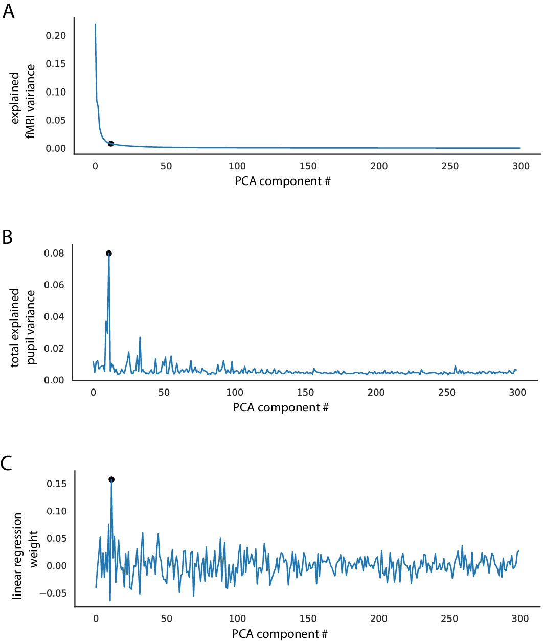
PCA decoupling of pupil-related fMRI activity from other signal sources.
(A) fMRI variance explained by individual PCA components. Components are ordered by variance explained. Black dot marks the component with the most explained pupil variance. (B) Pupil variance explained by the PCA signals. Same ordering as in (A). The component explaining the most pupil variance (explained var. = 7.03%) explains only 0.8% of fMRI variance. Black dot marks the component with the most explained pupil variance. (C) Weights of the linear regression model trained to decode pupil signals based on fMRI-PCA data. Each weight corresponds to a single PCA component’s time course. The highest absolute weights are not assigned to the components explaining the most fMRI variance. Black dot marks the component with the most explained pupil variance.
-
Figure 3—figure supplement 2—source data 1
The variance explained values (AB) and linear regression weights (C) are available in the source data file.
- https://cdn.elifesciences.org/articles/68980/elife-68980-fig3-figsupp2-data1-v2.zip
Figure 3—figure supplement 3
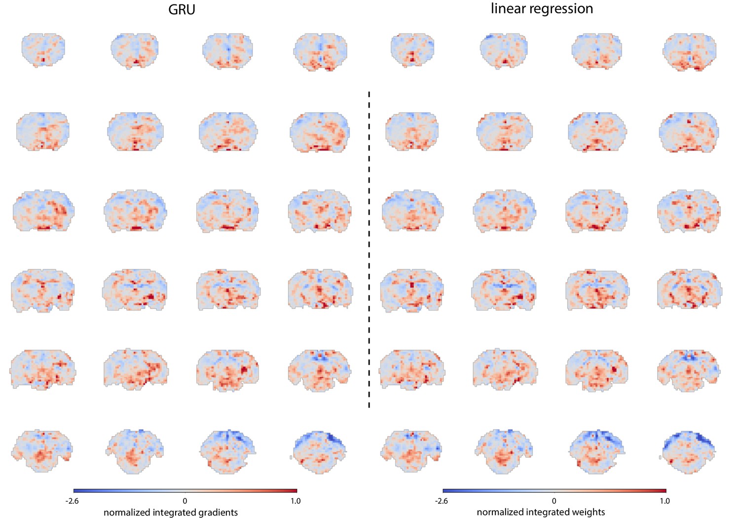
Similarity of GRU and linear regression prediction maps.
Spatial maps were generated by integrating PCA spatial maps with either linear regression weights or average GRU gradients. The maps highlight the same areas. This observation coupled with the similarity of predictions generated by both methods and the short GRU training time suggests that a linear mapping was sufficient for this decoding task.
-
Figure 3—figure supplement 3—source data 1
The maps are available in the source data file.
- https://cdn.elifesciences.org/articles/68980/elife-68980-fig3-figsupp3-data1-v2.zip
Figure 4
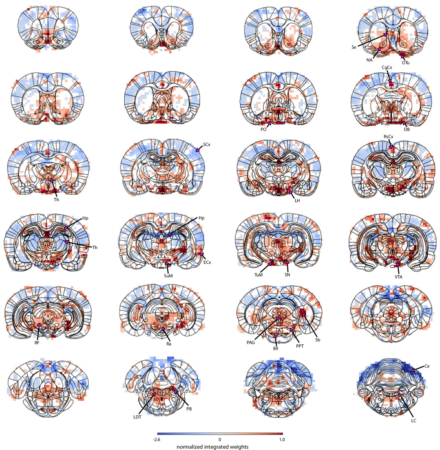
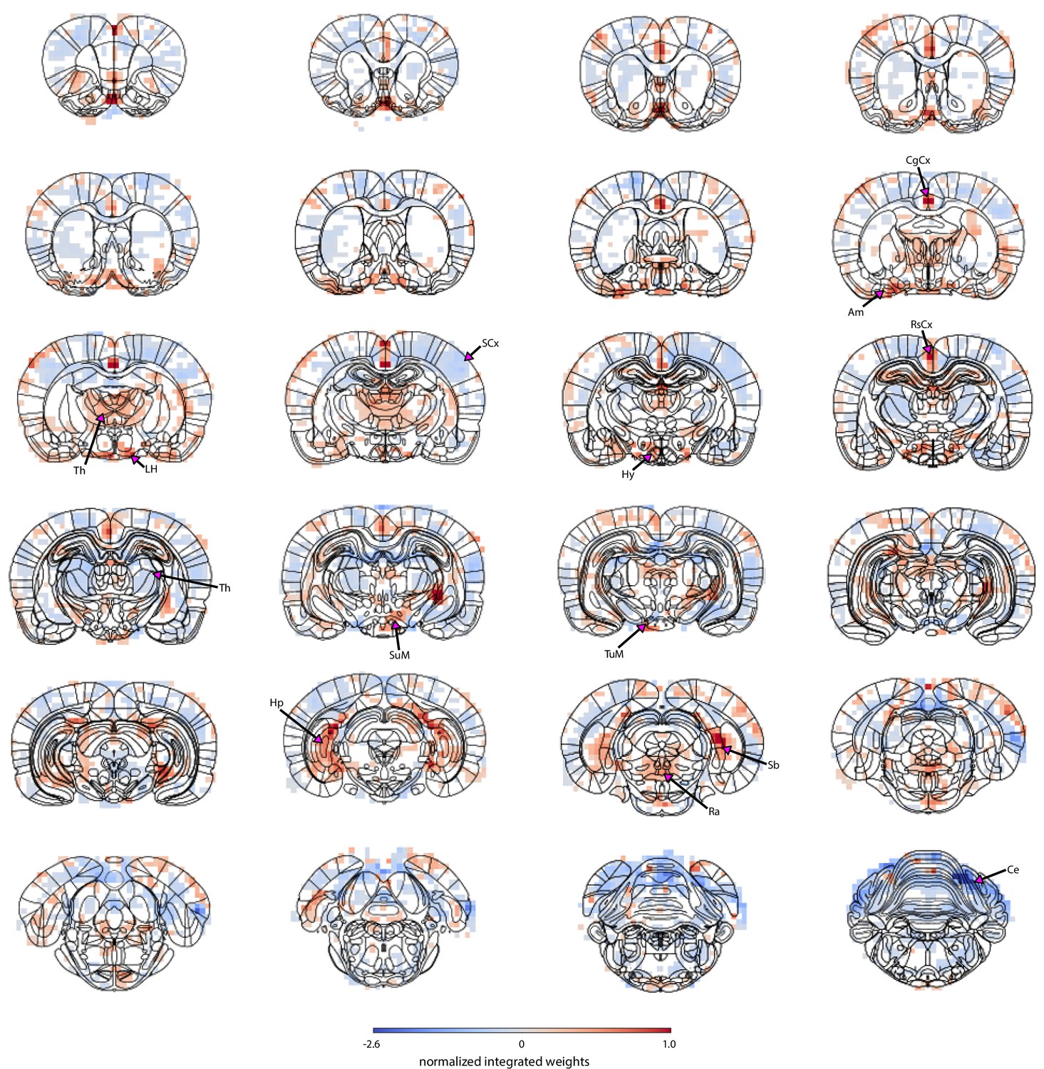
Localization of pupil dynamics-related information content across the brain.
The spatial map highlights regions from which pupil-related information was decoded. It was created by integrating PCA spatial maps with weights of the trained linear regression model. The map displays positive weights in all neuromodulatory regions of the ascending reticular activating system as well as in other regions involved in autonomous regulation – the lateral and preoptic hypothalamus and the periaqueductal gray. The subcortical basal forebrain nuclei (the horizontal limb of the diagonal band, nucleus accumbens, and olfactory tubercle) and the septal area were also positively coupled to pupil dynamics. Finally, regions of the hippocampal formation – the hippocampus, entorhinal cortex and subiculum, as well as cingulate, retrosplenial and visual cortices showed positive weights. The thalamus and the hippocampus had both positive and negative weights. Strong negative weighting was found in the cerebellum and most somatosensory cortical regions. Masked regions (white) did not pass the false discovery rate corrected significance threshold (p=0.01). Abbreviations: B9 – B9 serotonergic cells, Ce – cerebellum, CgCx – cingulate cortex, DB – horizontal limb of the diagonal band, ECx – entorhinal cortex, Hp – hippocampus, LC – locus coeruleus, LDT – laterodorsal tegmental nuclei, LH – lateral hypothalamus, NA – nucleus accumbens, OTu – olfactory tubercle, PAG – periaqueductal gray, PB – parabrachial nuclei, PO – preoptic nuclei, PPT – pedunculopontine tegmental nuclei, Ra – raphe, RF – reticular formation, RsCx – retrosplenial cortex, Sb – subiculum, SCx – somatosensory cortex, Se – septal nuclei, SN – substantia nigra, SuM – supramammillary nucleus, Th – thalamus, TuM – tuberomammillary nucleus, VTA – ventral tegmental area.
-
Figure 4—source data 1
The masked map is available in the source data file.
- https://cdn.elifesciences.org/articles/68980/elife-68980-fig4-data1-v2.zip
Figure 5 with 4 supplements
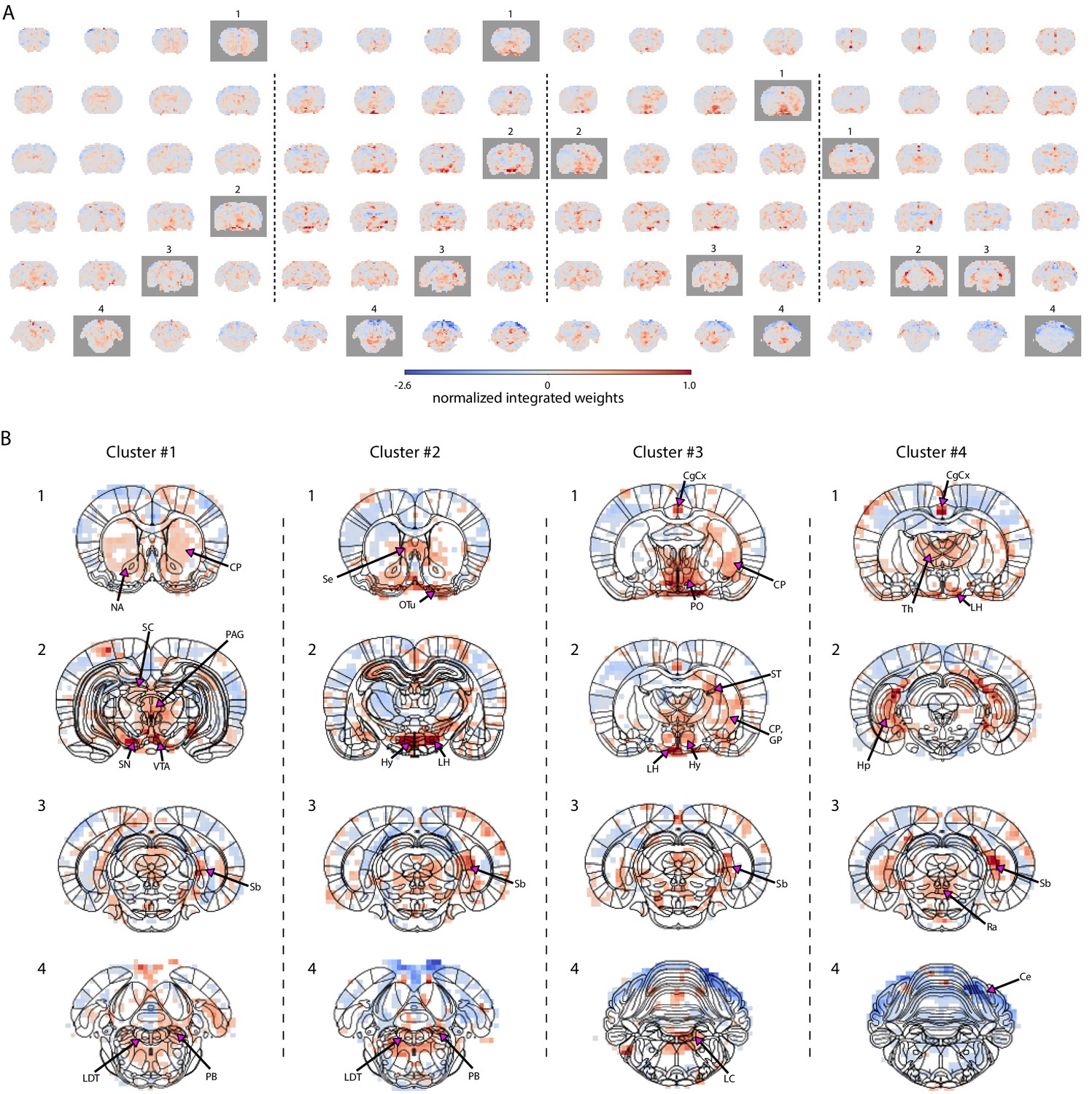
Characterization of brain state-specific pupil–fMRI relationships.
(A) Pupil information content maps generated by integrating PCA spatial maps with weights of linear regression models trained on cluster-specific trials. In all clusters, negative weights were found in the somatosensory cortex, the cerebellum, and posterior parts of the thalamus. All clusters had positive weights in anterior thalamic, preoptic and hypothalamic nuclei, subiculum, parts of the hippocampus and in the region containing the tuberomammillary nucleus. Clusters 1–3 displayed positive weights in neuromodulatory brainstem regions, substantia nigra, and ventral tegmental area, as well as the entorhinal cortex. The cingulate cortex and retrosplenial cortex and supramammillary nucleus were positive in clusters 2–4. Marked with gray are frames plotted in (B). (B) Cluster-specific spatial patterns are portrayed on slices selected from A (marked with gray rectangles). Characteristic to cluster 1 were positive weights in the dopaminergic substantia nigra and ventral tegmental area as well as in their efferent projections in the nucleus accumbens and caudate-putamen. Positive weighting was also found in the periaqueductal gray and brainstem laterodorsal tegmental and parabrachial nuclei, as well as in the superior colliculus. Cluster 2 was characterized by the strongest positive weights in hypothalamic regions, lateral in particular. Brainstem areas containing the arousal-regulating locus coeruleus, laterodorsal tegmental, and parabrachial nuclei, as well as the septal area and the olfactory tubercle displayed high positive weights. In cluster 3, as in cluster 2, the area containing the locus coeruleus, laterodorsal tegmental, and parabrachial nuclei showed positive linkage with pupil dynamics. The highest cluster 3 values were located in preoptic and other hypothalamic areas, as well as in stria terminalis carrying primarily afferent hypothalamic fibers, caudate-putamen, and globus pallidus. In cluster 4, the neuromodulatory region showing the strongest positive weights was the caudal raphe. The anterior parts of the brainstem displayed negative weighting. Characteristic to cluster 4 were high weights in the thalamus and in the hippocampus and the subiculum forming the hippocampal formation. Masked regions (white) did not pass the false discovery rate corrected significance threshold (p=0.01). Abbreviations: Ce – cerebellum, CgCx – cingulate cortex, CP – caudate-putamen, GP – globus pallidus, Hp – hippocampus, Hy – hypothalamus, LC – locus coeruleus, LDT – laterodorsal tegmental nuclei, LH – lateral hypothalamus, NA – nucleus accumbens, OTu – olfactory tubercle, PAG – periaqueductal gray, PB – parabrachial nuclei, PO – preoptic nuclei, Ra – raphe, Sb – subiculum, SC – superior colliculus, Se – septal area, SN – substantia nigra, ST – stria terminalis, Th – thalamus, VTA – ventral tegmental area.
-
Figure 5—source data 1
The unmasked cluster maps (A) and the masked maps based on randomization tests with a different random seed (B) are available in the source data file.
- https://cdn.elifesciences.org/articles/68980/elife-68980-fig5-data1-v2.zip
Figure 5—figure supplement 1
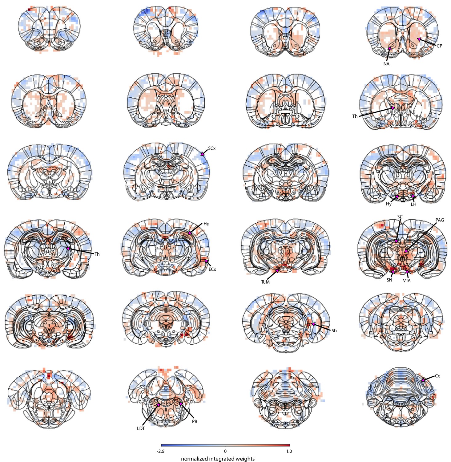
The spatial map based on cluster 1 trials highlights regions from which pupil-related information was decoded.
Masked regions (white) did not pass the false discovery rate corrected significance threshold (p=0.01). Abbreviations: Ce – cerebellum, CP – caudate-putamen, ECx – entorhinal cortex, Hp – hippocampus, Hy – hypothalamus, LDT – laterodorsal tegmental nuclei, LH – lateral hypothalamus, NA – nucleus accumbens, PAG – periaqueductal gray, PB – parabrachial nuclei, Sb – subiculum, SC – superior colliculus, SCx – somatosensory cortex, SN – substantia nigra, Th – thalamus, TuM – tuberomammillary nucleus, VTA – ventral tegmental area.
Figure 5—figure supplement 2
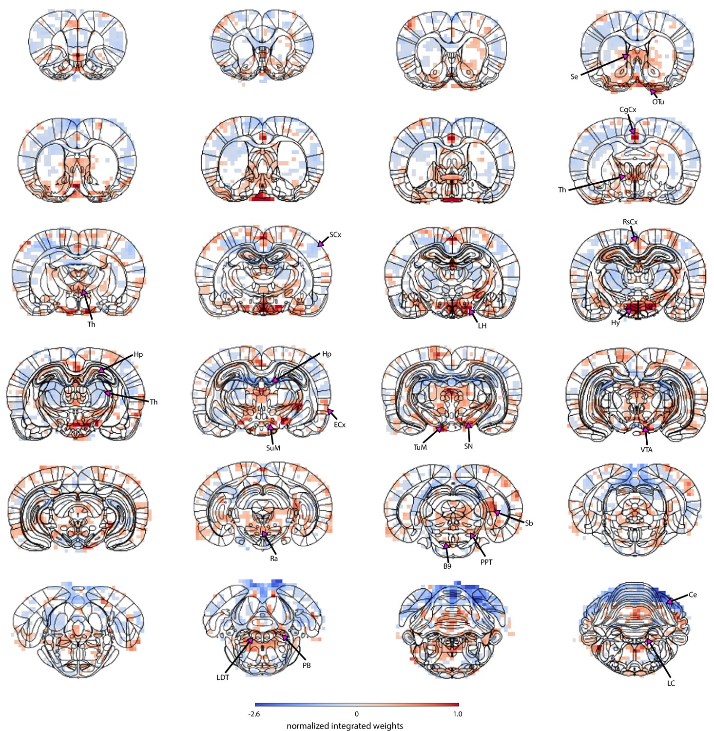
The spatial map based on cluster 2 trials highlights regions from which pupil-related information was decoded.
Masked regions (white) did not pass the false discovery rate corrected significance threshold (p=0.01). Abbreviations: B9 – B9 serotonergic cells, Ce – cerebellum, CgCx – cingulate cortex, ECx – entorhinal cortex, Hp – hippocampus, Hy – hypothalamus, LC – locus coeruleus, LDT – laterodorsal tegmental nuclei, LH – lateral hypothalamus, OTu – olfactory tubercle, PB – parabrachial nuclei, PPT – pedunculopontine tegmental nuclei, Ra – raphe, RsCx – retrosplenial cortex, Sb – subiculum, SCx – somatosensory cortex, Se – septal nuclei, SN – substantia nigra, SuM – supramammillary nucleus, Th – thalamus, TuM – tuberomammillary nucleus, VTA – ventral tegmental area.
Figure 5—figure supplement 3
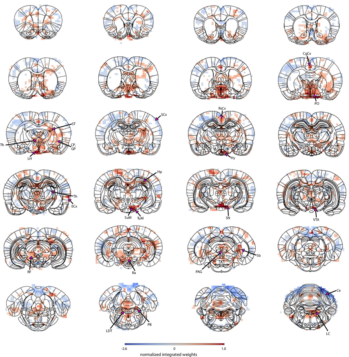
The spatial map based on cluster 3 trials highlights regions from which pupil-related information was decoded.
Masked regions (white) did not pass the false discovery rate corrected significance threshold (p=0.01). Abbreviations: Ce – cerebellum, CgCx – cingulate cortex, CP – caudate-putamen, ECx – entorhinal cortex, GP – globus pallidusHp – hippocampus, LC – locus coeruleus, LDT – laterodorsal tegmental nuclei, LH – lateral hypothalamus, PAG – periaqueductal gray, PB – parabrachial nuclei, PO – preoptic nuclei, Ra – raphe, RF – reticular formation, RsCx – retrosplenial cortex, Sb – subiculum, SCx – somatosensory cortex, SN – substantia nigra, ST – stria terminalis, SuM – supramammillary nucleus, Th – thalamus, TuM – tuberomammillary nucleus, VTA – ventral tegmental area.
Figure 5—figure supplement 4
The spatial map based on cluster 4 trials highlights regions from which pupil-related information was decoded.
Masked regions (white) did not pass the false discovery rate corrected significance threshold (p=0.01). Abbreviations: Ce – cerebellum, CgCx – cingulate cortex, Hp – hippocampus, LH – lateral hypothalamus, Ra – raphe, RsCx – retrosplenial cortex, Sb – subiculum, SCx – somatosensory cortex, SuM – supramammillary nucleus, Th – thalamus, TuM – tuberomammillary nucleus.
Tables
Table 1
Optimized GRU hyperparameters.
| Parameter name | Description | Range | Final value |
|---|---|---|---|
| Number of layers | Multiple recurrent layers could be stacked on top of each other. | [1; 3] | 1 |
| Hidden size | Hidden state vector size. | [10; 500] | 300 |
| Learning rate | The rate at which network weights were updated during training. | [10–6; 1] | 0.0023 |
| L2 | Strength of the L2 weight regularization. | [0; 10] | 0.0052 |
| Gradient clipping | Gradient clipping (Pascanu et al., 2013) limits the gradient magnitude at a specified maximum value. | [yes; no] | Yes |
| Max. gradient | Value at which the gradients are clipped. | [0.1, 2] | 1 |
| Dropout | During training, a percentage of units could be set to 0 for regularization purposes (Srivastava et al., 2014). | [0; 0.2] | 0 |
| Residual connection | Feeding the input directly to the linear decoder bypassing the RNN’s computation. | [yes; no] | No |
| Batch size | The number of training trials fed into the network before each weight update. | [3; 20] | 12 |
Additional files
Download links
A two-part list of links to download the article, or parts of the article, in various formats.
Downloads (link to download the article as PDF)
Open citations (links to open the citations from this article in various online reference manager services)
Cite this article (links to download the citations from this article in formats compatible with various reference manager tools)
Decoding the brain state-dependent relationship between pupil dynamics and resting state fMRI signal fluctuation
eLife 10:e68980.
https://doi.org/10.7554/eLife.68980


