Causal roles of prefrontal cortex during spontaneous perceptual switching are determined by brain state dynamics
- International Research Centre for Neurointelligence, The University of Tokyo Institutes for Advanced Study, Japan
- RIKEN Centre for Brain Science, Japan
Figures
Figure 1
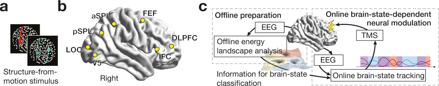
Experiment design.
While the participants were presented with a structure-from-motion (SFM) stimulus (a), we recorded EEG signals from the seven brain regions (b). DLPFC, dorsolateral prefrontal cortex; IFC, inferior frontal cortex; FEF, frontal eye fields; aSPL/pSPL, anterior/posterior superior parietal lobule; LOC, lateral occipital complex. In the control experiments, we first conducted offline energy landscape analysis, whose results allowed us to categorise brain activity patterns into either of the three major brain states (c, left). By implementing such classification information to an online EEG analysis, we tracked brain state dynamics and administered inhibitory TMS in state-/state-history-dependent manners (c, right).
Figure 2
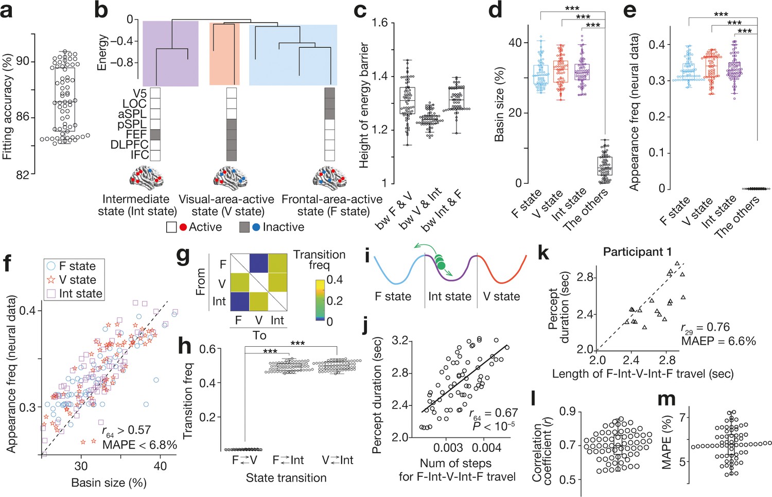
Feasibility of energy landscape analysis for EEG data.
(a-d) We confirmed that the brain state dynamics found in the EEG data were qualitatively the same as those seen in our previous fMRI study (Watanabe et al., 2014c). A pairwise maximum entropy model, a basis for the energy landscape analysis, was accurately fitted to the EEG data (a) and yielded almost the same energy landscape structure with three major brain states (e.g. panel b for Participant 1). The three brain states were significantly separated with high energy barriers (c) and dominated almost all the energy surface (d). (e and f) These estimations based on the energy landscape structure were consistent with the actual neural data. In the EEG data, almost all the neural activity patterns could be categorised into either of the three major brain states (e). The basin sizes in the model accurately predicted the appearance frequency of the major brain states (f; each mark represents each individual). (g–j) We then performed random-walk simulations on the energy landscape and found that there was no direct transition between F and V state (panel g for the group average of the transition matrix; panel h for the transition frequencies for all the participants). This result suggests that, during the bistable visual perception, the neural activity pattern (a green ball in panel i) is travelling between F and V state via Int state (i). As shown in our fMRI work, the number of steps to complete this F-Int-V-Int-F travel was correlated with the behavioural percept duration across participants (j). (k–m). We confirmed that this brain-behaviour correlation was seen at an individual level. Technically, for each run in a participant, we calculated the length of the neural travel between F and V state via Int state and compared it with the percept duration for the run. Panel k shows such a comparison in Participant 1, indicating a significant correlation between the brain state dynamics and perceptual stability in the participant. In the other participants, these associations were preserved (panel l for the correlation coefficients; panel m for the mean average per cent error, MAPE). In the panels a, c-e, h, j, l and m, dots represent participants. ***, P < 10–3 in a paired t-test (df = 64).
Figure 3
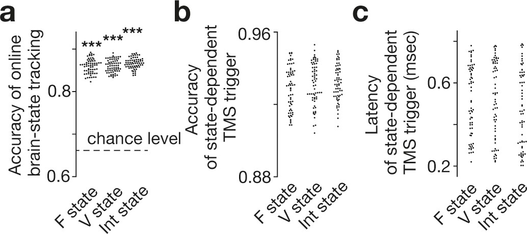
Accuracy of online brain state tracking and triggering of TMS.
The online EEG analysis tracked brain state dynamics as accurately as the offline analysis did (a). Brain-state-dependent TMS triggering system also achieved accurate neural tracking (b) with short delays (c). Note that the accuracy in the TMS trigger (b) tended to be higher than that in simple brain-state tracking (a), presumably because TMS was triggered only when a specific brain state was expected to continue in a certain period (here, 150 ms) and resultantly reduce the rate of false negative. Also, such a criterion should work as temporal smoothing and improve the signal-to-noise ratio. Each dot represents each participant. *** indicates PBonferroni <0.001 in paired t-tests (df = 64).
Figure 4
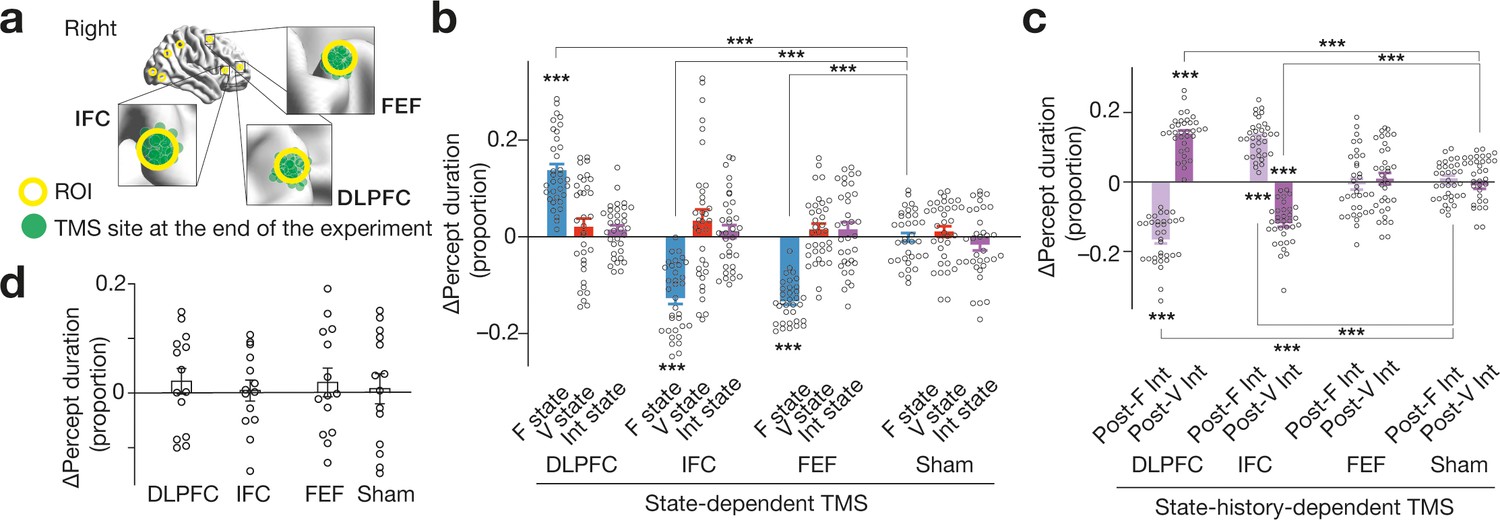
Behavioural results .
(a) We administered inhibitory TMS over the three PFC regions. In one TMS condition, we placed the TMS coil over one of the PFC areas using a stereoscopic neuro-navigation system based on the MNI coordinates at the beginning of each experiment day. At the end of the day, we re-measured the coordinates of the TMS coil using the navigation system. Finally, we averaged the coordinates across the 4-day sessions in the main experiment. The green circles represent such mean MNI coordinates of the stimulated brain site for each participant. The green circles were mapped closely onto the original coordinates (the centres of the yellow circles). (b) State-dependent TMS revealed that causal behavioural roles of the three PFC regions are detectable when the brain activity pattern stays in F state. The Y-axis shows the proportional changes in the median percept duration ( = (TMS–control)/control). The X-axis indicates the TMS conditions. *** indicates PBonferroni <0.001 in paired t-tests (df = 33). Each circle represents each participant. The error bars show the s.e.m. (c) The DLPFC and IFC showed state-history-dependent behavioural causal effects on bistable visual perception, while FEF did not. *** indicates PBonferroni <0.001 in paired t-tests (df = 33). (d) No significant behavioural change was induced after stronger and longer TMS (30min quadripulse TMS with 90 % AMT) over the same three PFC regions. The error bars show the s.e.m.The intensity of the current TMS was set at 70 % AMT.
Figure 5

Effects on energy landscape structure .
We numerically simulated how inhibitory TMS would affect the heights of the F-to-Int, Int-to-F, Int-to-V and V-to-Int barrier for each participant (a), which predicted significant changes in the energy barriers (panel b for TMS over DLPFC, panel c for TMS over IFC and panel d for TMS over FEF). In the panels b-d, the solid tricolour curves schematically represent post-TMS energy landscape structures, whereas the dashed curves denote the original energy landscape. *** indicates PBonferroni <0.001 in paired t-tests (df = 33). The error bars show the s.e.m.
Figure 6
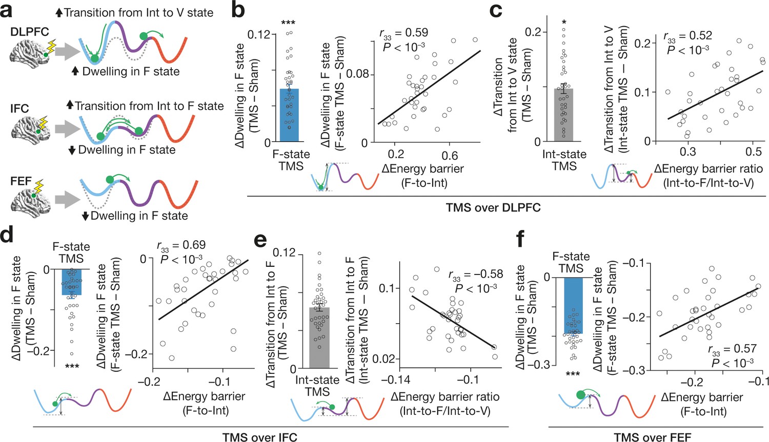
Effects on brain state dynamics.
(a) The numerical simulation (Figure 5) enables us to infer TMS-induced effects on the brain state dynamics. The tricolour curves schematically indicate the energy landscapes modified by TMS, whereas the dashed curves show the original energy landscapes. The green circles show the brain activity pattern. (b–f) These inferences were empirically confirmed. The X-axes show the changes in the hypothetical energy barrier heights, whereas the Y axes indicate TMS-induced neural effects on the brain state dynamics. The circles represent the participants. *** and * indicate PBonferroni <0.001 and PBonferroni <0.05 in paired t-tests (df = 33), respectively. The error bars show the s.e.m.
Figure 7
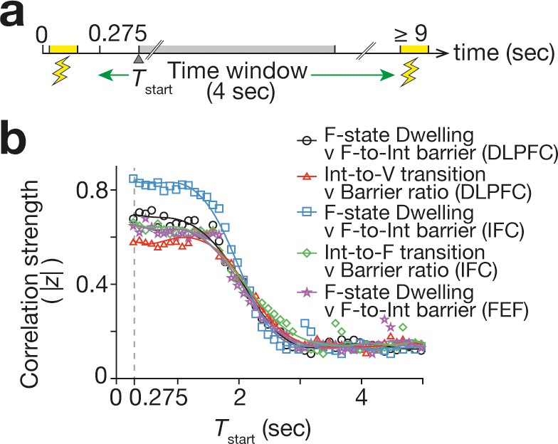
Duration of TMS effects.
To assess the duration of the TMS-induced neural effects, we examined how the correlations seen in Figure 6 changed when we slided the 4 s time window that was used to measure the neural effects. In all the correlations, the correlation strength (here, the absolute value of the Fisher-transformed correlation coefficient, |z|) began to decay ~1.5 s after the TMS. The X-axis shows the start timing of the 4 s time window (Tstart).
Figure 8
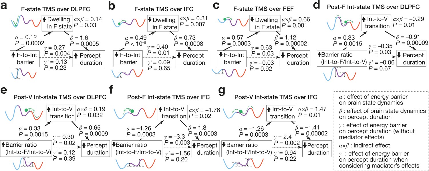
Associations between energy landscape structure, brain state dynamics and behaviour.
The mediation analyses showed that the structural changes in the energy landscapes affect the brain state dynamics, which results in the causal behavioural responses. The statistical significance of the α, β, and γ validate our application of the mediation analysis to the current data. The statistical significance of the α⨉β and the insignificance of the γ’ support the conclusions.
Figure 9

Validation tests.
(a) All the main behavioural causal responses were replicated in an independent cohort (N = 14). (b) In another independent experiment (N = 15), we administered excitatory TMS over the same PFC regions. The excitatory stimulaton induced behavioural effects opposite to those seen in the inhibitory TMS experiments. Each circle represents each participant. *** and ** indicate P < 0.001 and P < 0.01 in one-sample t-tests (df = 13 for panel a and df = 14 for panel b), respectively. The error bars show the s.e.m.
Figure 10
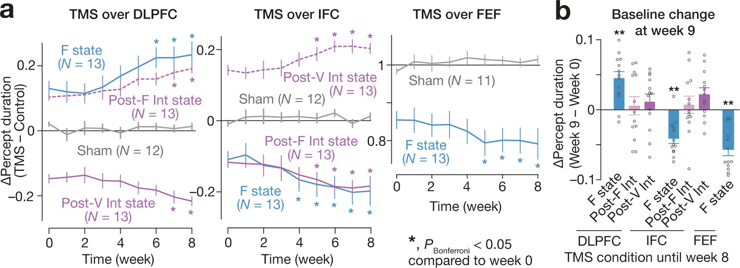
Long-term effects.
We found the accumulative effects of the state-/state-history-dependent TMS on the bistable visual perception in 2-month longitudinal experiments (a). We focused on the seven TMS conditions that induced significant behavioural effects (Figure 4b,c). Even after the 2-month weekly TMS experiments, we observed significant changes in the baseline percept duration in three of the seven TMS conditions (b). In panel a, the Y-axes show the changes in the median percept duration (TMS – Control), and * indicates PBonferroni <0.05 in paired t-tests with comparisons to the week-0 values (df = 12). In panel b, the Y-axis indicates the changes in the control performance between week 0 and 9. ** indicates PBonferroni <0.01 in one-sample t-tests (df = 12).
Figure 11
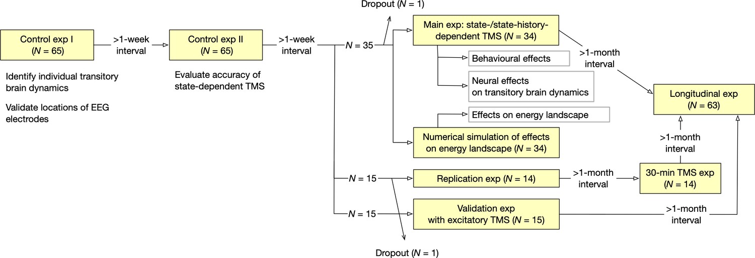
Oveall study design.
The current study consisted of seven EEG/TMS experiments and one numerical simulation.
Figure 12
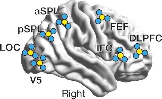
Location of electrodes.
We placed TMS-compatible EEG electrodes in an original way. First, seven electrodes were located right above on the seven ROIs using a stereoscopic neuro-navigation system. Then, for each ROI, three additional electrodes were placed right around the electrodes for the following Hjorth signal calculation. The yellow circles schematically represent the electrodes put above the ROIs, whereas the blue ones indicate the neighbouring electrodes.
Figure 13
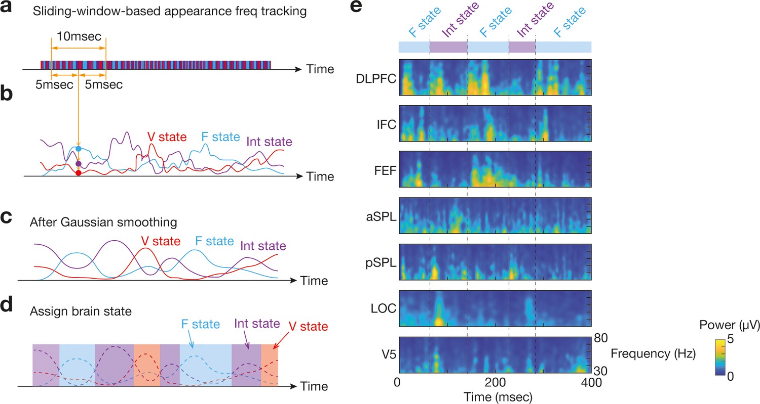
Identification of brain state dynamics.
To reduce the effects of noise-oriented fluctuation in bran state dynamics, we applied two temporal smoothing procedures to the original brain state dynamics data. First, in a sliding window manner, we calculated three appearance frequency values for the three brain states (a and b). Then, Gaussian temporal smoothing was applied to the three appearance frequency curves (c). By comparing the smoothed curves, we identified which brain state was the most dominant at each timepoint (d). Panel e shows an example for such brain state transitions with time-frequency plots of the seven ROIs in Participant 1.
Figure 14
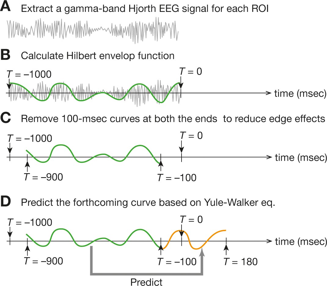
Online EEG preprocessing .
For the online preprocessing of EEG data, we first calculated a Hjorth EEG signal from each ROI data and then extracted a gamma-band signal in a sliding-window manner (a). Next, we fitted the Hilbert envelop function (b) and removed both ends of the 1000 ms time window to reduce the edge effects (c). Finally, based on the remaining 800 ms Hilbert envelop function, we made the prediction of the forthcoming 280 ms signal (d). Such 280 ms signals would be used for brain-state tracking.
Figure 15
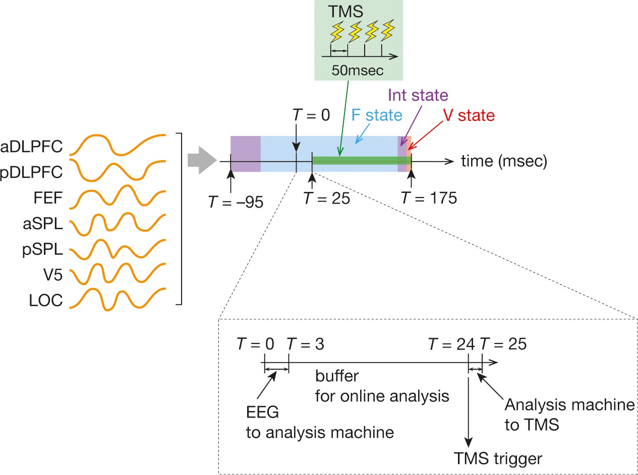
Timings of TMS.
After the online preprocessing, we obtained seven time-series data for the seven ROIs (orange curves in the left). We put the seven ROI signals into binarisation, brain state categorisation and temporal smoothing procedures, which resulted in brain state dynamics in the 270 ms time period (T = –95 to T = 175 ms). When one brain state dominated the time window, the online analysis machine sent a trigger at T = 24 ms after a 21 ms buffer period (a dashed box in the bottom). A burst of the inhibitory TMS consisted of three TMS stimulations with 500 msec intervals and thus took 150 ms (green box in the centre).
Figure 16
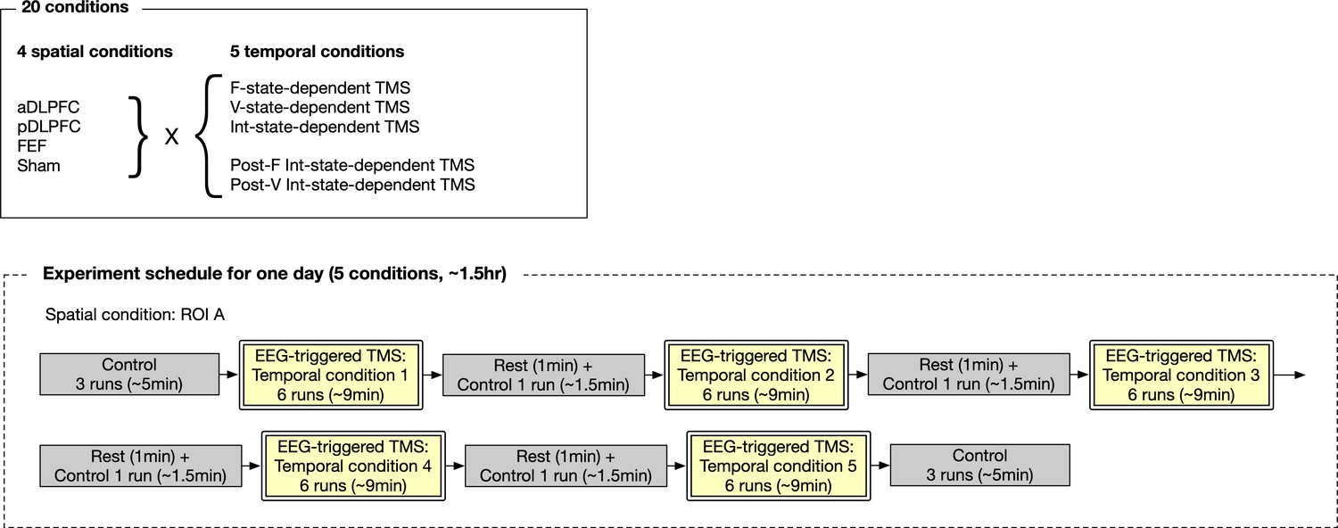
Design of the main experiment.
For each participant, the experiment was conducted over four different days with> one week intervals. On each day, they received TMS/sham over one of the three PFC days in five different timings. The stimulation site for the sham condition was randomly chosen from the three PFC areas and balanced across the participants.
Figure 17
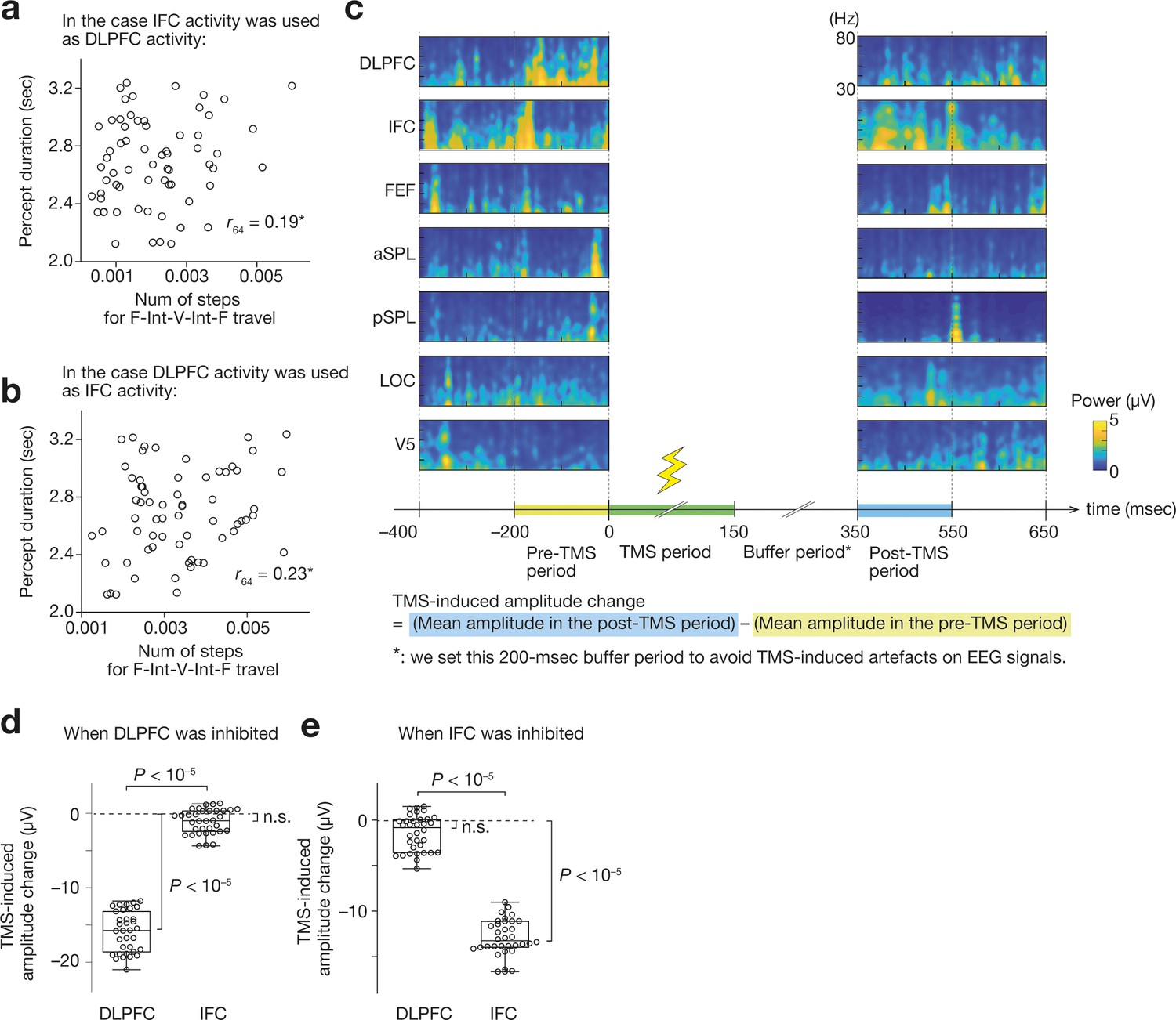
Spatial sensitivity and specificity of the current EEG system.
(a and b) If we replaced one of the prefrontal activities with the other, the brain-behaviour association in the original result (Figure 2j) deteriorated. Panel a shows a result when the DLPFC activity was replaced with the IFC activity. Panel b shows a correlation when the IFC activity was set as the same value as the DLPFC activity. *, Z > 3.2, p < 0.0018 in the comparison of the brain-behaviour correlation between the original one and one after the operation to replace one prefrontal activity with the other. Each circle represents each participant. (c) We investigated the TMS-induced changes in the gamma-band amplitude. For example, the panel c shows the gamma-band signals for the seven ROIs before and after a TMS administration over the DLPFC in Participant 1. We calculated the mean amplitude of the gamma-band signals in both pre-TMS and post-TMS periods and estimated the neural effects of the TMS. (d and e) When we applied TMS over the DLPFC, the DLPFC activity was significantly reduced but the IFC activity was not (panel d). When the TMS was performed over the IFC, only the IFC activity was inhibited (panel e). Each circle represents each participant.
Figure 18
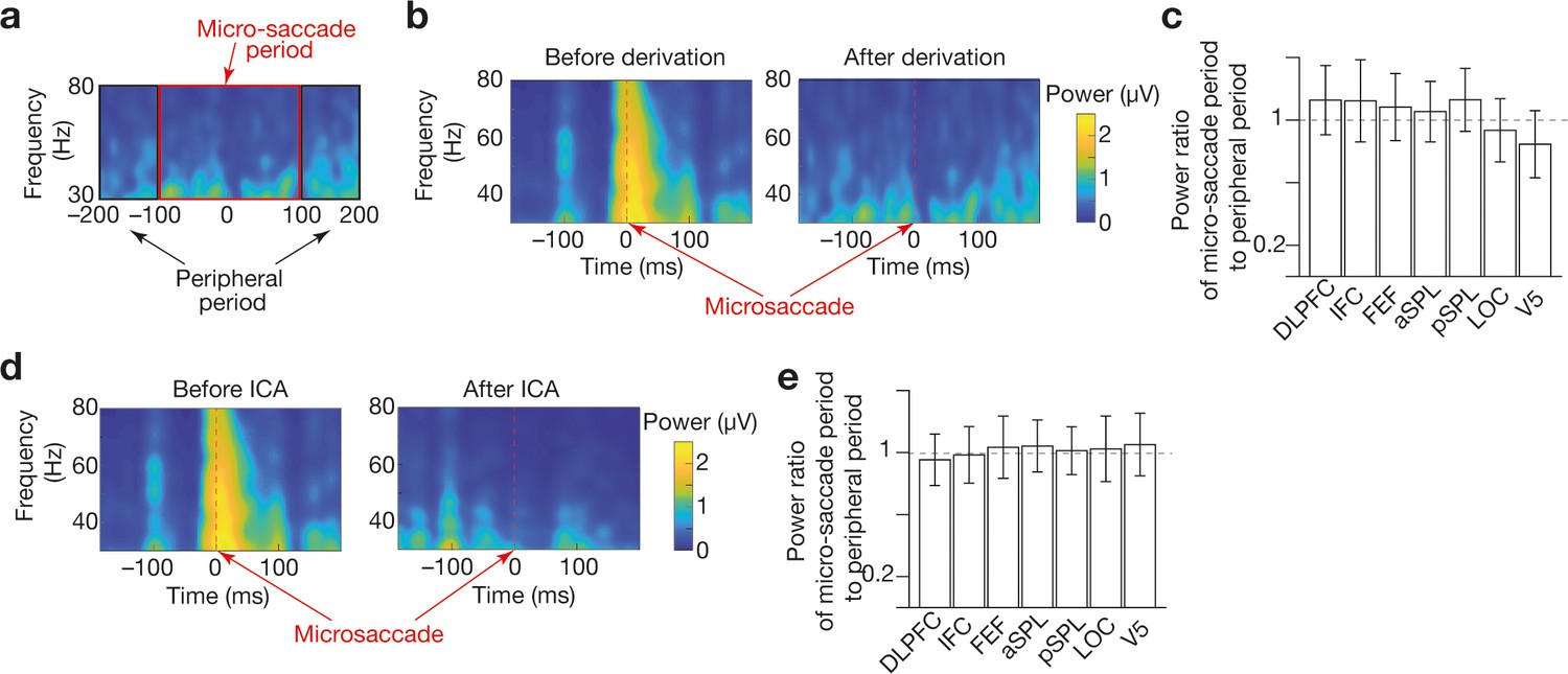
Preprocessing to reduce microsaccade-relevant effects on EEG data .
We adopted a derivation method (Keren et al., 2010; Pulvermüller et al., 1997; Trujillo et al., 2005; Zion-Golumbic et al., 2010) and independent component analysis (ICA) (Hassler et al., 2011; Jung et al., 2000; Lee et al., 1999) to reduce the artefacts of microsaccades on gamma-band EEG signals. To evaluate the effectiveness of these methods, we compared the mean amplitudes of the gamma-band signals between the microsaccade and peripheral period (a). The timings of microsaccades were determined based on EOG signals (Croft and Barry, 2000; Elbert et al., 1985; Keren et al., 2010; Shan et al., 1995). The derivation method was able to reduce the artefacts of the microsaccades (panel b for an example of IFC signals in Participant 1) in all the seven regions of interest (ROIs; panel c). The ICA could also substantially weaken such effects (panel d for an example of IFC signals in Participant 1) in all the seven ROIs (e).
Additional files
Download links
A two-part list of links to download the article, or parts of the article, in various formats.
Downloads (link to download the article as PDF)
Open citations (links to open the citations from this article in various online reference manager services)
Cite this article (links to download the citations from this article in formats compatible with various reference manager tools)
Causal roles of prefrontal cortex during spontaneous perceptual switching are determined by brain state dynamics
eLife 10:e69079.
https://doi.org/10.7554/eLife.69079


