Persistent cell migration emerges from a coupling between protrusion dynamics and polarized trafficking
- Laboratoire Physico Chimie Curie, Institut Curie, PSL Research University, Sorbonne Université, France
- Cell Biology and Cancer Unit, Institut Curie, PSL Research University, Sorbonne University, France
- Faculty of Science and Engineering, Sorbonne Université, France
- Institut Curie, PSL Research University, France
- Tumor Cell Dynamics Unit, Gustave Roussy Institute, Université Paris-Saclay, France
Figures
Figure 1 with 2 supplements
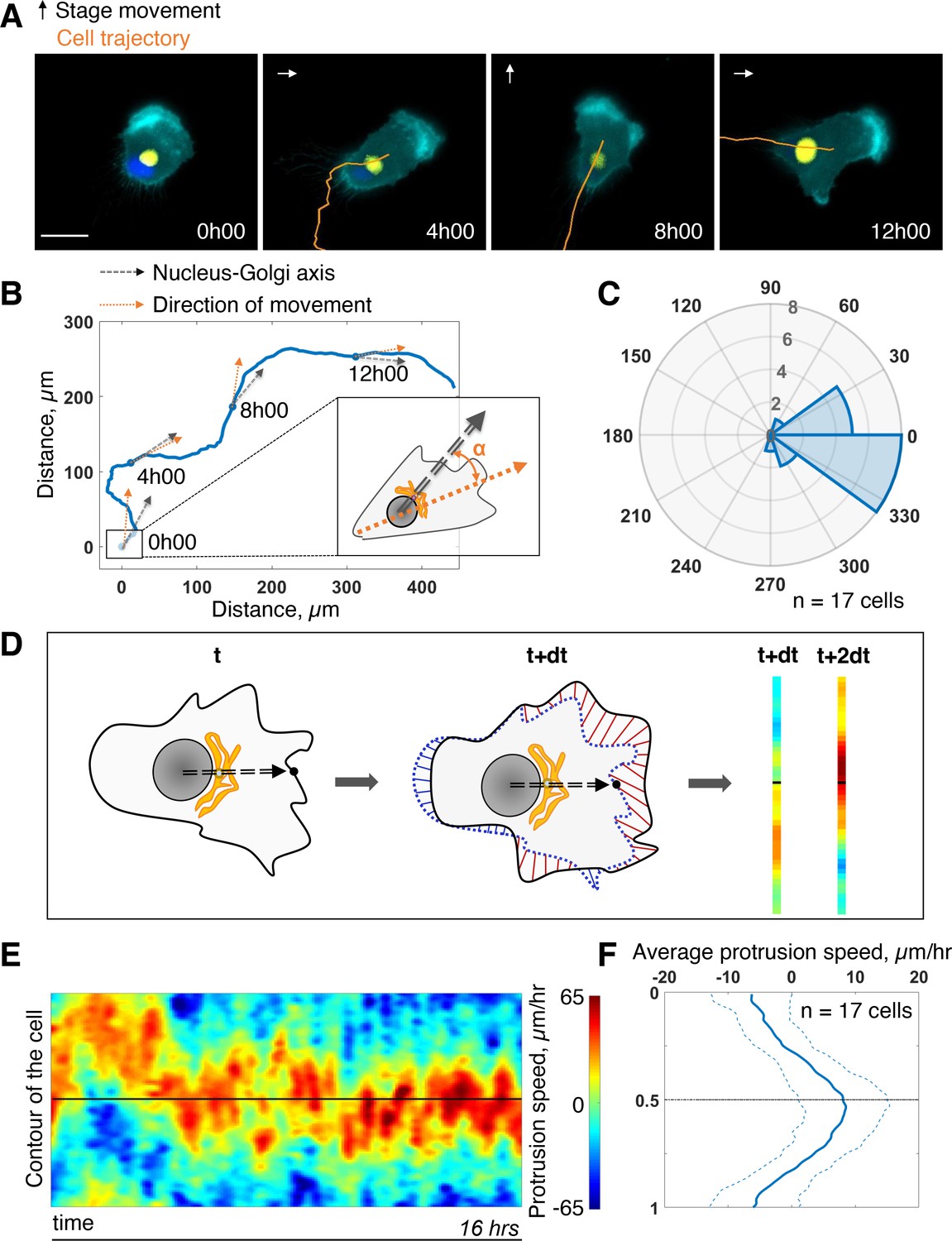
Persistent protrusions form in front of the Golgi complex.
(A) Snapshots of a representative migrating RPE1 cell at different timepoints tracked with a feedback routine in which the microscope stage follows a migrating cell (Figure 1—figure supplement 1) for 16 hr (cyan: myr-iRFP, yellow: GFP-Rab6A, blue: Hoechst 33342, trajectory overlaid in orange, microscope stage movement represented by an arrow, scale bar – 20 µm). (B) Full trajectory of a representative cell shown in (A) with Nucleus-Golgi (black dashed arrow) and direction of movement (orange dashed arrow) axes overlaid. (C) Polar histogram representing the averaged angle between Nucleus-Golgi axis and direction of movement (n = 17 cells). (D) Explanatory sketch of how a morphodynamic map of cell shape changes is computed. The contour of the cell is extracted and compared between frames and stretched out to a line representation, where the distance traveled by a point in the contour is represented (red color meaning protrusion, blue – retraction, black dashed arrow – Nucleus-Golgi axis). (E) Morphodynamic map of a representative cell (all maps in Figure 3—figure supplement 2) recentered to Nucleus-Golgi axis (black). X-axis represents time and Y-axis represents cell contour. (F) Average protrusion speed over time (n = 17 cells, dashed blue line - SD). X-axis represents average protrusion speed, and Y- axis represents cell contour with the midline corresponding to (E). Data used for C and F and related scripts can be found in Figure 1—source data 1.
-
Figure 1—source data 1
Data and analysis scripts with explanations for Figure 1 and its supplements.
- https://cdn.elifesciences.org/articles/69229/elife-69229-fig1-data1-v2.zip
Figure 1—figure supplement 1
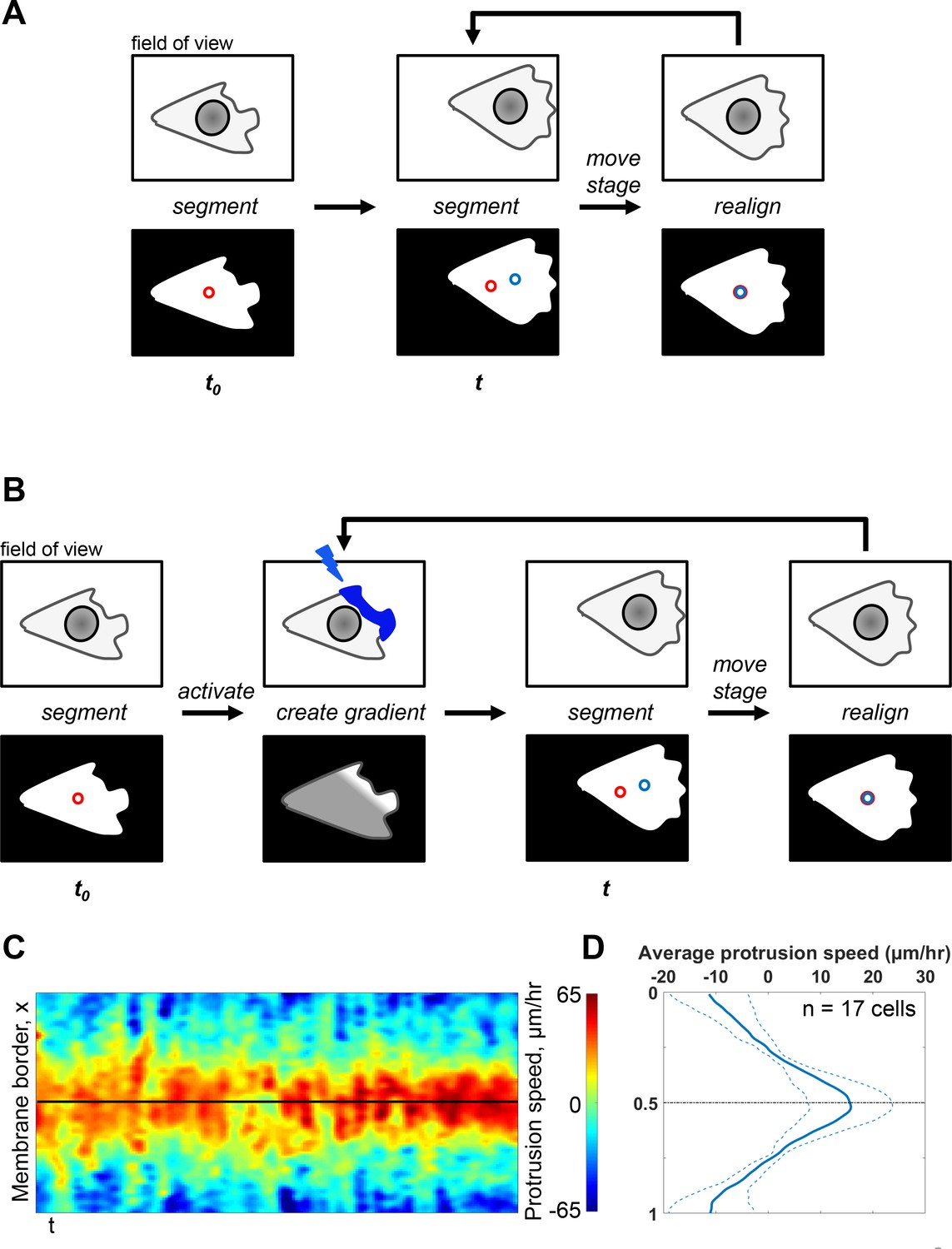
Feedback routine for moving the microscope stage (field of view) to follow a migrating cell.
(A) First frame (t0) - centroid of a cell (red circle) found from a segmented image; following frame (t) - new centroid of a cell (blue circle) is found from a taken image at time t, if the two centroids are further than a defined distance, the microscope stage is moved and two centroids are aligned. This routine continues until the end of experiment. (B) Specific light activation can be included in the feedback routine, where activation pattern is automatically adapted to the shape of the cell and goes along the plasma membrane border with selected pattern thickness. (C) Morphodynamic map of a representative cell recentered to direction of movement (black). (D) Average protrusion speed over time (n = 17 cells, dashed blue line - SD). Data used for C-D and related scripts can be found in Figure 2—source data 1.
Figure 1—video 1
Human telomerase reverse transcriptase (hTERT)–immortalized RPE1 cell freely moving on a fibronectin covered coverslip followed by a moving microscope stage.
RPE1 cell freely moving on a fibronectin (2 µg/mL) covered coverslip followed by a moving microscope stage (cyan: myr-iRFP, yellow: Rab6A, blue: Hoechst 33342, trajectory overlaid in orange, scale bar – 20 µm, time resolution – 5 min.)
Figure 2 with 3 supplements
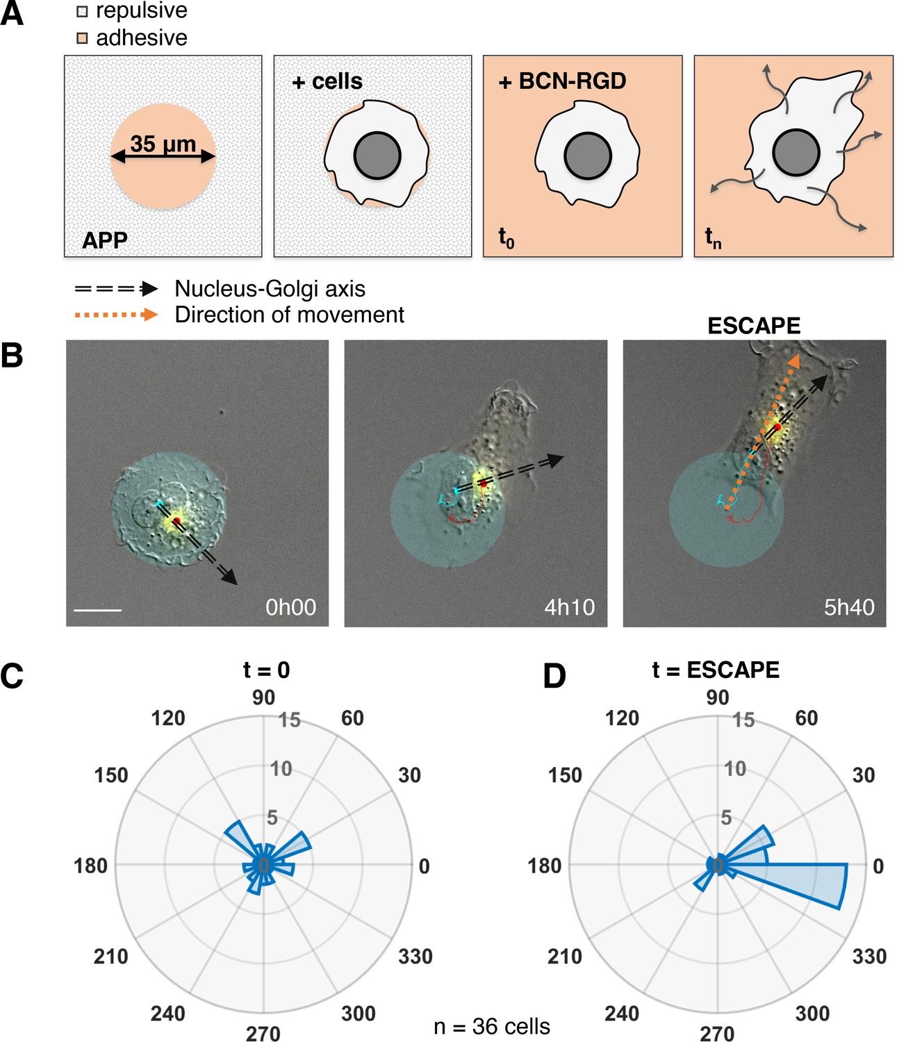
Nucleus-Golgi axis and direction of movement align when a cell starts moving.
(A) Scheme of the dynamic micropatterns experimental design that is used to study the initiation of cell movement. A cell is confined on a round fibronectin pattern and after the addition of BCN-RGD is enabled to move outside and ‘escape’ the pattern (‘escape’ is defined to be the moment when the center of the cell nucleus is leaving the area of the pattern). (B) Representative RPE1 cell ‘escaping’ the pattern (transparent cyan: pattern, cyan dot: nucleus centroid, yellow: GFP-Rab6A, red dot: Golgi centroid, black dashed line: Nucleus-Golgi axis, orange dashed line: direction of movement, scale bar – 20 µm). (C–D) Polar histograms representing the angle between Nucleus-Golgi axis at the beginning of experiment (t = 0) (C) or at the time of ‘escape’ (t = ESCAPE) (D) and direction of movement when the cell moves out of the pattern (n = 36 cells). Data used for C and D and related scripts can be found in Figure 2—source data 1.
-
Figure 2—source data 1
Data and analysis scripts with explanations for Figure 2 and its supplements.
- https://cdn.elifesciences.org/articles/69229/elife-69229-fig2-data1-v2.zip
Figure 2—figure supplement 1

Detailed analysis of Nucleus-Golgi axis movement when a cell is escaping the pattern.
Change in position of Nucleus-Golgi axis while moving out of an isotropic pattern (white circle: pattern, a line represents evolution of Nucleus-Golgi axis position in time from blue (start of experiment) to red (end of experiment), movement aligned by the author for visual purposes).
Figure 2—figure supplement 2

Detailed analysis of Nucleus-Golgi axis movement when a cell is escaping the pattern.
(A) Distance of the nucleus centroid from the center of the pattern. The nucleus starts to move out of the center approximately 1 hr before the escape. Its movement clearly points to the moment when the cell goes out of the pattern (black arrow) (time resolution – 10 min). Time is normalized for each cell by the time of escape (defined as t = 0 here). (B) Nucleus-Golgi axis position is roughly established at the same time as direction of movement (notice the orange and black arrows pointing to the start of the slope). Evolution of Nucleus-Golgi axis position and cell movement (orange: direction of movement, defined as Nucleus-center of the pattern axis, black: Nucleus-Golgi axis, the position of both axes is normalized by the direction of movement at the time of ‘escape’ from the pattern (orange curve goes to zero) (n = 36 cells), time resolution – 10 min). Data used for A-B and related scripts can be found in Figure 2—source data 1.
Figure 2—video 1
RPE1 cell ‘escaping’ the pattern.
RPE1 cell ‘escaping’ the pattern (scale bar – 20 µm, time resolution – 10 min).
Figure 3 with 5 supplements

Low dose of Nocodazole (NZ) reduces persistence of migration.
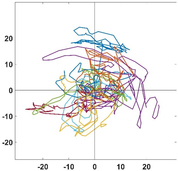
(A–B) Representative morphodynamic maps of RPE1 cells freely moving on a fibronectin-covered coverslip in control condition (Ctrl) (A) and with NZ (0.1 µm) (B). (C–E) Average protrusion speed (C), average cell speed (D), and directionality ratio (E) compared in Ctrl and with NZ (Wilcoxon rank sum test, *p≤0.05, **p≤0.01, ***p≤0.001). (F–G) Trajectories of RPE1 cells in Ctrl (n = 17) (F) and with NZ (n = 14) (G) (trajectories plotted over 7 hr of experiment). (H–I) Direction autocorrelation (H), and persistence time (I) compared in Ctrl and with NZ (Wilcoxon rank sum test, *p≤0.05, **p≤0.01, ***p≤0.001). Data used for C-I and related scripts can be found in Figure 3—source data 1.
-
Figure 3—source data 1
Data and analysis scripts with explanations for Figure 3 and its supplements.
- https://cdn.elifesciences.org/articles/69229/elife-69229-fig3-data1-v2.zip
Figure 3—figure supplement 1

Low concentrations of Nocodazole (NZ) slow down microtubule (MT) dynamics without significantly changing the MT network content.
(A) Representative images of immunofluorescence staining of α-Tubulin (MTs) and DNA (nucleus) in fixed RPE1 cells with addition of 0.1 μM NZ and in control conditions (DMSO) after 1 hr, 3 hr, 6 hr, and 24 hr (DMSO condition: 1 hr – n = 17 cells; 3 hr – n = 6 cells; 6 hr – n = 5 cells; 24 hr – n = 14 cells; NZ condition: 1 hr – n = 15 cells; 3 hr – n = 24 cells; 6 hr – n = 17 cells; 24 hr – n = 18 cells; scale bar – 20 μm). (B) Representative image of live imaging of α-Tubulin-GFP (MTs) in RPE1 cells with addition of 0.1 uM NZ and in control conditions (DMSO) after 3 hr (DMSO condition – n = 8 cells; NZ condition – n = 8 cells; scale bar – 20 μm). (C) Image of one frame and a max projection of EB3-GFP ( + end of MTs) comet trajectories of a 2 min video (acquisition every 1 s) in RPE1 cells with addition of 0.1 uM NZ and in control conditions (DMSO) after 3 hr (DMSO condition – n = 17 cells; NZ condition – n = 31 cells; scale bar – 20 μm).
Figure 3—figure supplement 2

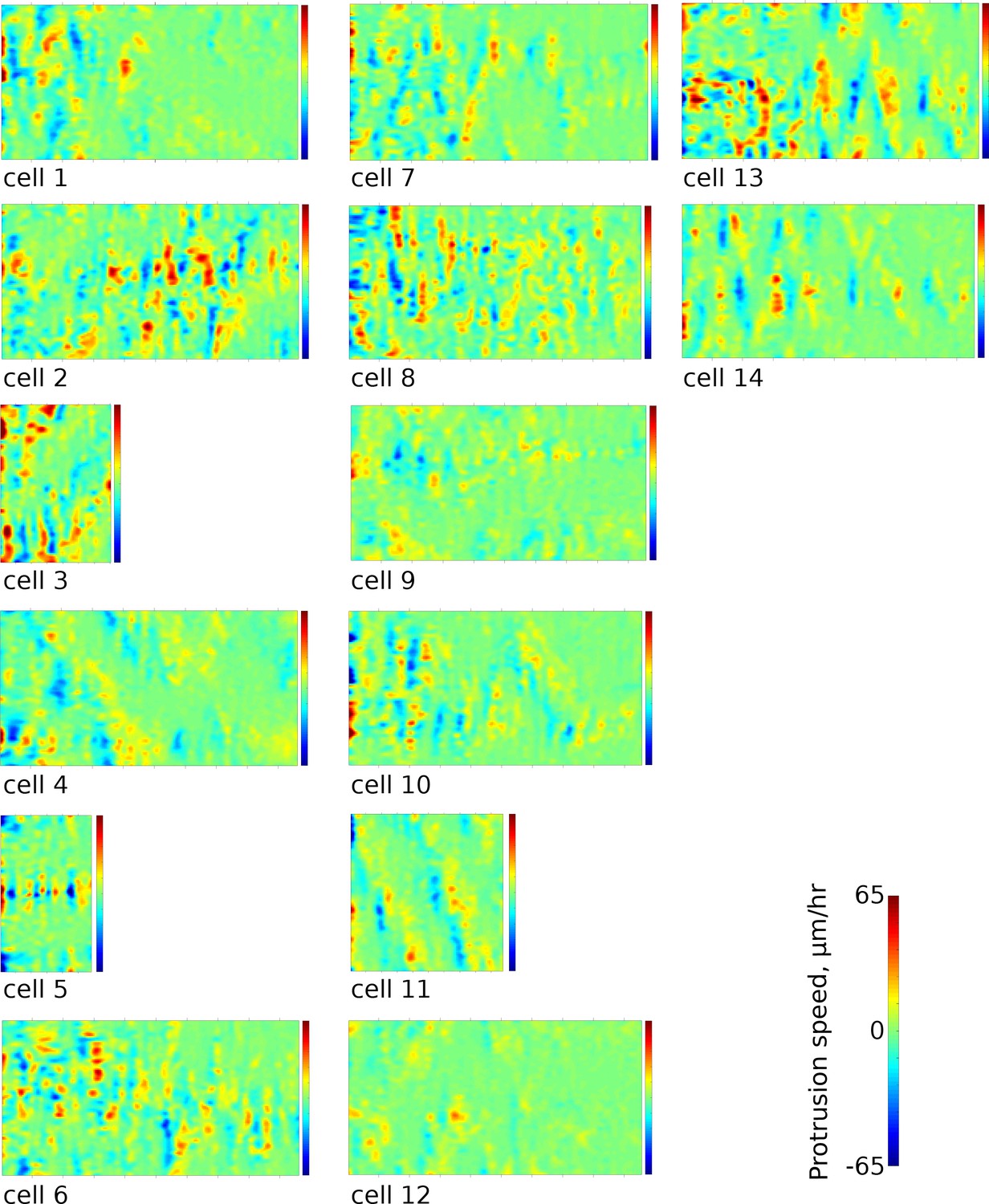
All morphodynamic maps from control experiments.
Raw morphodynamic map data can be found in Figure 3—source data 1.
Figure 3—figure supplement 3
All morphodynamic maps from Nocodazole experiments.
Raw morphodynamic map data can be found in Figure 3—source data 1.
Figure 3—video 1
RPE1 cell freely moving in 2D in control conditions and with Nocodazole (0.1 μM).
RPE1 cell freely moving on a fibronectin (2 µg/mL) covered coverslip followed by a moving microscope stage in control conditions (A) and with Nocodazole (0.1 µM) (B) (scale bar – 20 µm, time resolution – 5 min).
Figure 3—video 2
Microtubule dynamics in RPE1 cells in control conditions and with Nocodazole (0.1 μM).
RPE1 cells labeled with EGFP-α-Tubulin (A) and with EGFP-EB3 (B, lower panel) in control conditions and with Nocodazole (0.1 µM) (scale bar – 20 µm, time resolution – 1 s).
Figure 4 with 5 supplements
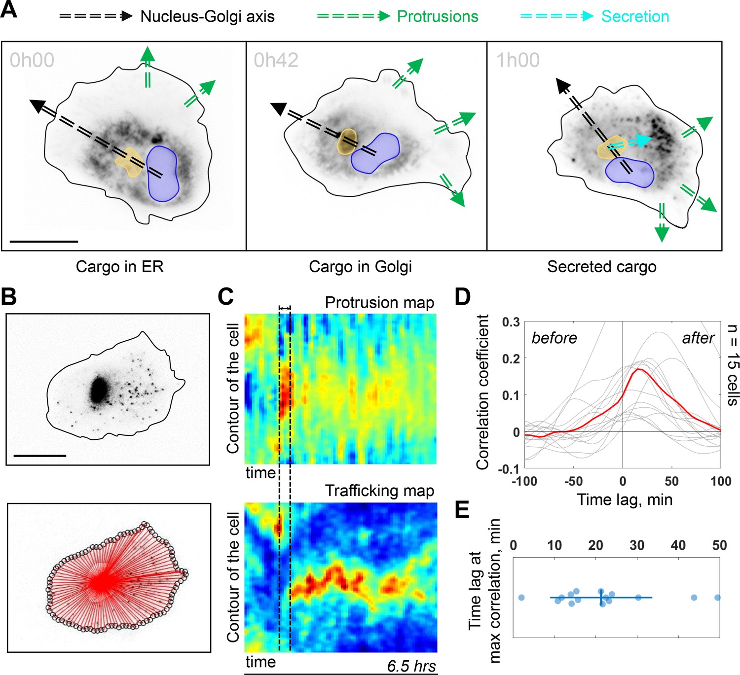
Trafficking from Golgi complex is biased toward the protrusion.
(A) Collagen X cargo (labeled in black) is traveling from ER to the Golgi complex and secreted during a Retention Using Selective Hooks assay experiment (blue contour: nucleus, yellow contour: Golgi complex, green dashed line: protrusions, black dashed line: Nucleus-Golgi axis, cyan dashed line: secretion axis, scale bar - 20 μm). (B) Top, RPE1 cells expressing endogenous levels of a marker for post-Golgi vesicles (iRFP-Rab6A) (scale bar - 20 μm). Bottom, red lines represent the lines over which vesicle traffic intensity is calculated over time. (C) Top, a representative morphodynamic map representing plasma membrane protrusions in time. Bottom, a representative trafficking map showing the flow of post-Golgi vesicles from the Golgi complex along straight lines toward the surface over time time period - 6.5 hr, black dashed lines represent the time difference between a spike in protrusions (top) and a spike in secretion (bottom). X-axis represents time and Y-axis represents the contour of the cell. (D) Cross-correlation coefficient between plasma membrane protrusions and secretion as a function of the time lag (n = 15 cells, red line: average curve depicting the correlation coefficient, gray lines: single cell data; ‘before’ and ‘after’ denote the time before the protrusion peak and after, respectively). (E) Single cell time lags in minutes between protrusions and secretion at maximal correlation, obtained by fitting the peak of individual cross-correlation curves (gray curves in (D)). Data used for C-E and related scripts can be found in Figure 4—source data 1.
-
Figure 4—source data 1
Data and analysis scripts with explanations for Figure 4 and its supplements.
- https://cdn.elifesciences.org/articles/69229/elife-69229-fig4-data1-v2.zip
Figure 4—figure supplement 1

Examples of Retention Using Selective Hooks-SPI assays in control and Nocodazole conditions.
(A) Examples of secreted cargo being trafficked toward cellular protrusions in RPE1 cells. Secreted Col10A cargo signature on anti-GFP covered coverslip (green dashed line: protrusions, scale bar - 20 µm). (B) Examples of cargo secretion in the Nocodazole (0.1 uM) condition in RPE1 cells. Secreted Col10A cargo signature on anti-GFP covered coverslip (scale bar - 20 µm).
Figure 4—figure supplement 2
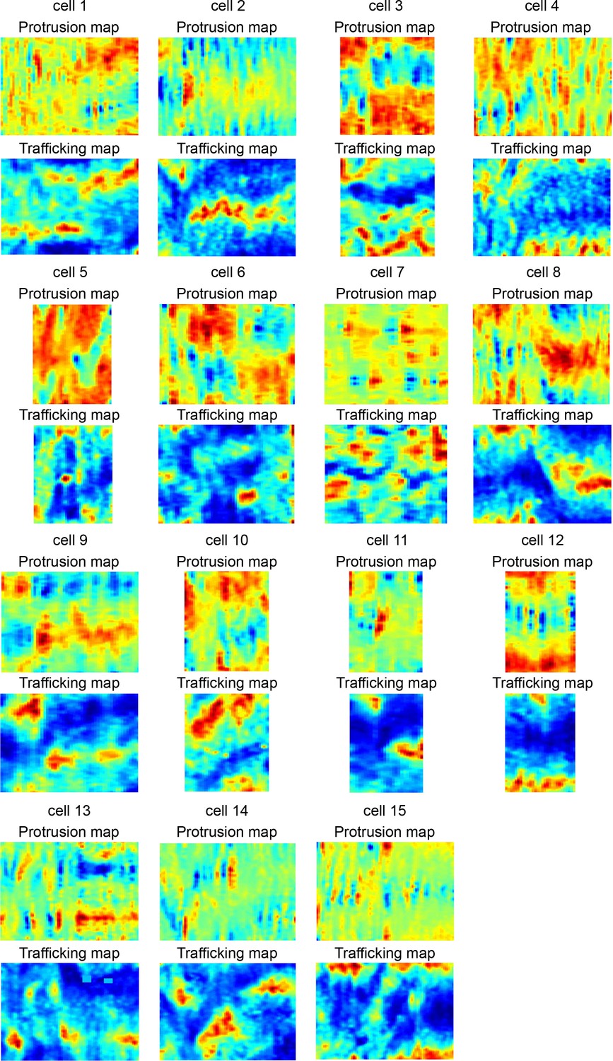
All protrusion and trafficking maps from trafficking experiments in control conditions.
Morphomap data can be found in Figure 4—source data 1.
Figure 4—figure supplement 3
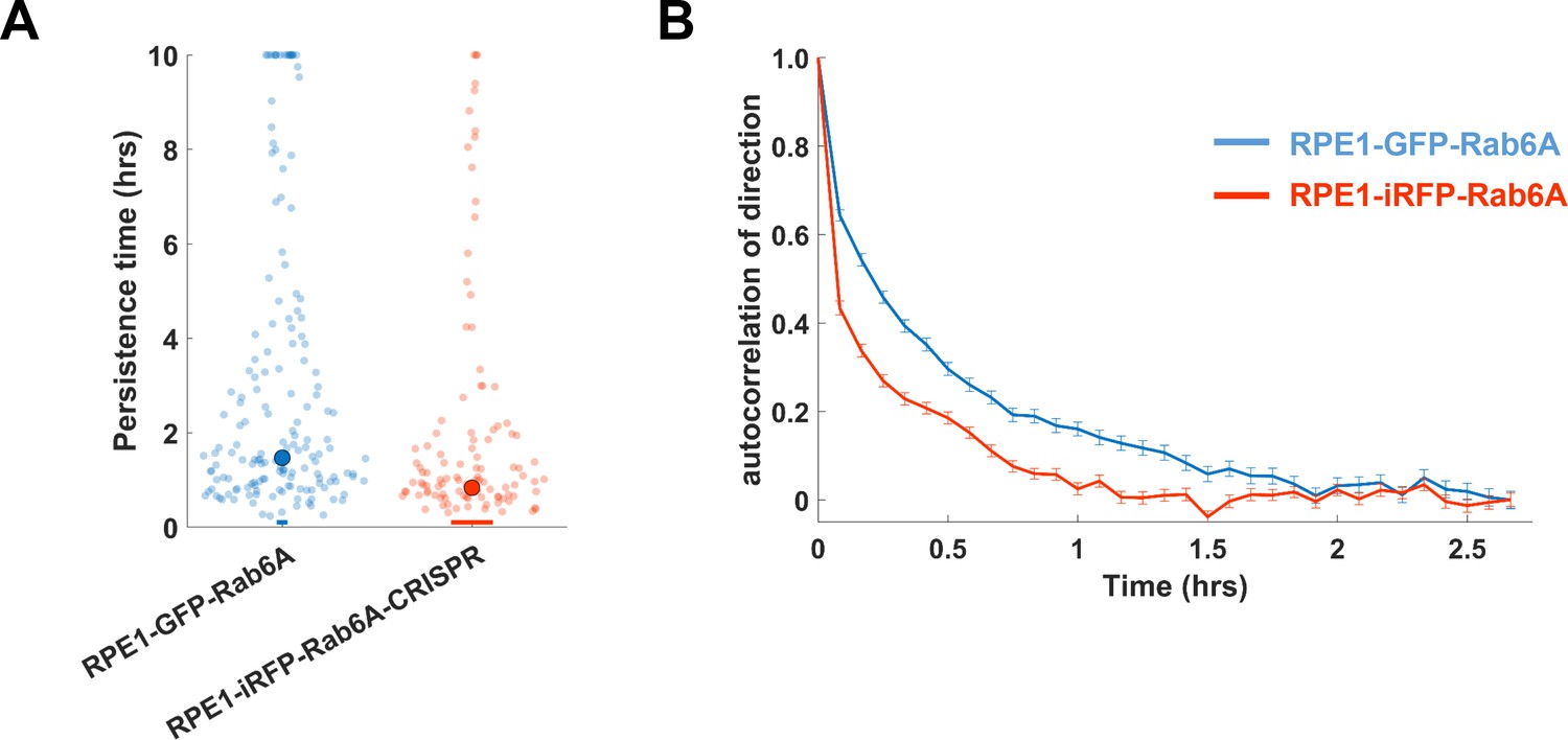
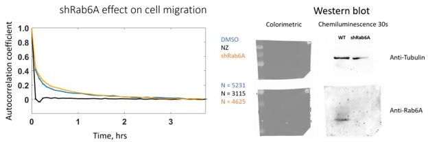
Comparison of persistence between Rab6 overexpression and Rab6 endogenous level.
(A–B) Analysis of 16-hr cell tracks using a 10× magnification. (A) Distribution of persistence time for the two conditions. The large dots represent the median of the distributions, and the horizontal lines - the fraction of nonpersistent cells. (B) Autocorrelation of cell direction as a function of time lag for the two conditions (RPE1-GFP-Rab6A overexpression N = 173, RPE1-iRFP-Rab6A endogenous expression N = 136). Data used and related scripts can be found in Figure 4—source data 1.
Figure 4—figure supplement 4

Large scale comparison of persistence for different drug conditions.
(A) Examples of 16-hr cell tracks (5 min time interval) using a Cytonote 6 W lensless microscope placed in an incubator for different experimental conditions. (B) Time over which the Golgi complex appears dispersed for increasing amounts of Golgicide A. Red box: chosen concentration of Golgicide A for further experiments. (C–E) Analysis of cell tracks from the Cytonote 6 W lensless microscope (three replicates of each condition). (C) Fraction of cells which are not persistent for each condition. Cells were defined as not persistent when their individually averaged autocorrelation of direction was below 0.3 at the first time lag. (D) Autocorrelation of cell direction as a function of time lag for each condition. (E) Distribution of persistence time for each condition. The large dots represent the median of the distributions, and the horizontal lines - the fraction of nonpersistent cells as in (C). Control n = 1681, DMSO n = 2201, Golgicide A n = 1292, Nocodazole n = 1692, Taxol n = 1641. Data used and related scripts can be found in Figure 4—source data 1.
Figure 4—video 1
RPE1 cells in Retention Using Selective Hooks (RUSH)-SPI assay with labeled Collagen X cargo in control and with Nocodazole, and with labeled Rab6A in control and with Nocodazole.
(A) RPE1 cell transfected with labeled Collagen X cargo (labeled in black) in control endoplasmic reticulum to the Golgi complex and is secreted during a RUSH assay experiment toward a newly forming protrusion (time resolution – 2 min, scale bar - 20 µm). (B) RPE1 cell transfected with labeled Collagen X cargo (labeled in black) treated with Nocodazole (0.1 µM) (time resolution – 2 min, scale bar - 20 µm). (C) RPE1 cell with labeled Rab6A (labeled in black) freely moving on a fibronectin (2 µg/mL) covered coverslip in control conditions (black arrow: Nucleus-Golgi axis, cyan arrow: secretion axis, scale bar – 20 µm, time resolution – 5 min). (D) RPE1 cell with labeled Rab6A (labeled in black) freely moving on a fibronectin (2 µg/mL) covered coverslip treated with Nocodazole (0.1 µM) (scale bar – 20 µm, time resolution – 5 min).
Figure 5 with 2 supplements
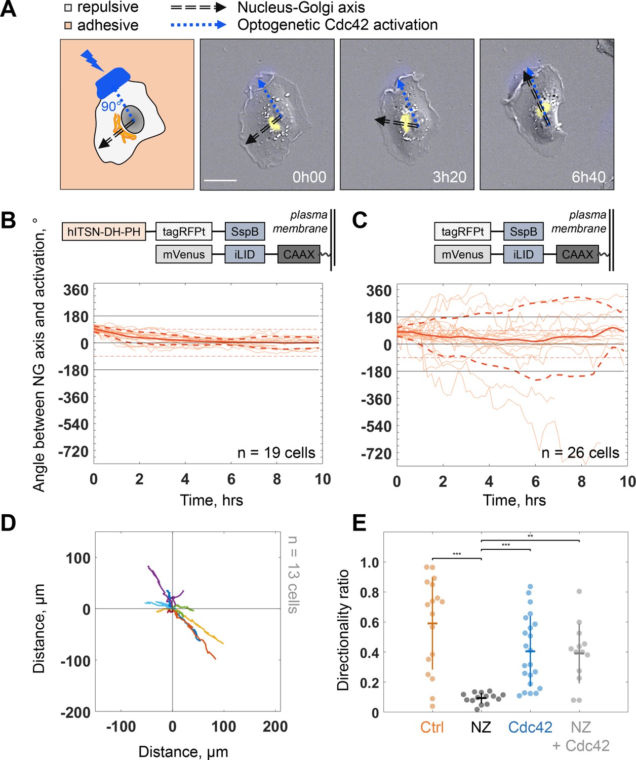
Biochemical gradient of Cdc42 reorients the Golgi complex and rescues directional migration.
(A) DIC image overlaid with Golgi marker (yellow, iRFP-Rab6A) of an RPE1 cell optogenetically activated 90° away from its initial Nucleus-Golgi axis (black dashed line: Nucleus-Golgi axis, blue dashed line: optogenetic activation axis, scale bar – 20 μm). (B–C) Optogenetic activation of Cdc42 90° away from Nucleus-Golgi axis leads to its reorientation in RPE1 cells freely moving on fibronectin covered coverslip (n = 19 cells) (B) and is random in control condition (n = 26 cells) (C) (thin orange lines: single cell data, thick orange line: data average, dashed thick orange lines: standard deviation; corresponding optogenetic constructs used are depicted above the graphs). (D) Trajectories of cells moving in this experimental condition (n = 13 cells; trajectories plotted over 7 hr of experiment). (E) Directionality ratio comparison between optogenetically activated cells in presence of Nocodazole (NZ) (orange: freely moving cells (‘Ctrl’, n = 17 cells), black: freely moving cells in presence of NZ (‘NZ’, n = 14 cells), blue: optogenetically activated cells (‘Cdc42’, n = 22 cells), gray: optogenetically activated cells in presence of NZ (‘NZ +Cdc42, n = 13 cells); Kruskal–Wallis test followed by a post hoc Dunn’s multiple comparison test, *p≤0.05, **p≤0.01, ***p≤0.001). Data used for B-E and related scripts can be found in Figure 5—source data 1.
-
Figure 5—source data 1
Data and analysis scripts with explanations for Figure 5 and its supplements.
- https://cdn.elifesciences.org/articles/69229/elife-69229-fig5-data1-v2.zip
Figure 5—figure supplement 1

Biochemical gradient of Cdc42 stabilizes the Golgi complex position and reorients it on an isotropic pattern.
(A) RPE1 cell, following the Nucleus-Golgi axis reorientation toward the optogenetically induced protrusion (yellow: iRFP-Rab6A, blue: optogenetic activation, black dashed line: Nucleus-Golgi axis, blue dashed line: optogenetic activation axis, scale bar – 20 µm). (B) Optogenetic activation of protrusion formation in front of existing Nucleus-Golgi axis leads to its stabilization in RPE1 cells freely moving on fibronectin covered coverslip (n = 19 cell; thin orange lines: single cell data, thick orange line: data average, dashed thick orange lines: standard deviation). (C) Cumulative graph, showing the ratio of cells, whose Nucleus-Golgi axis reorients in time (reorientation threshold - 30°, black: activation on pattern (n = 16 cells), orange: activation on free cells (n = 22 cells)). (D) RPE1 cell on a round fibronectin pattern (d = 35 µm), following the Nucleus-Golgi axis reorientation toward optogenetic activation of Cdc42 (yellow: iRFP-Rab6A, blue: optogenetic activation, black dashed line: Nucleus-Golgi axis, blue dashed line: optogenetic activation axis, scale bar – 20 µm). (E–F) Optogenetic activation of protrusion formation 90° away from Nucleus-Golgi axis leads to its reorientation in RPE1 cells on round fibronectin micropatterns (n = 16 cells) (E) and is random in control condition (n = 13 cells) (F) (thin orange lines: single cell data, thick orange line: data average, dashed thick orange lines: standard deviation). Data used for Figure 5B,C and E–F and related scripts can be found in Figure 5—source data 1.
Figure 5—video 1
RPE1 cells exposed to local optogenetic Cdc42 activation while freely moving, on a round pattern and freely moving with Nocodazole.
(A) RPE1 cell, following the Nucleus-Golgi axis reorientation toward the optogenetically induced protrusion (yellow: iRFP-Rab6A, blue: optogenetic activation, scale bar – 20 µm, time resolution – 10 min). (B) RPE1 cell on a round fibronectin pattern (d = 35 µm), following the Nucleus-Golgi axis reorientation toward optogenetic activation of Cdc42 (yellow: iRFP-Rab6A, blue: optogenetic activation, scale bar – 20 µm, time resolution – 10 min). (C) RPE1 cell, following the Nucleus-Golgi axis reorientation toward the optogenetically induced protrusion treated with Nocodazole (NZ, 0.1 µm) (yellow: iRFP-Rab6A, blue: optogenetic activation, scale bar – 20 µm, time resolution – 10 min).
Figure 6 with 4 supplements
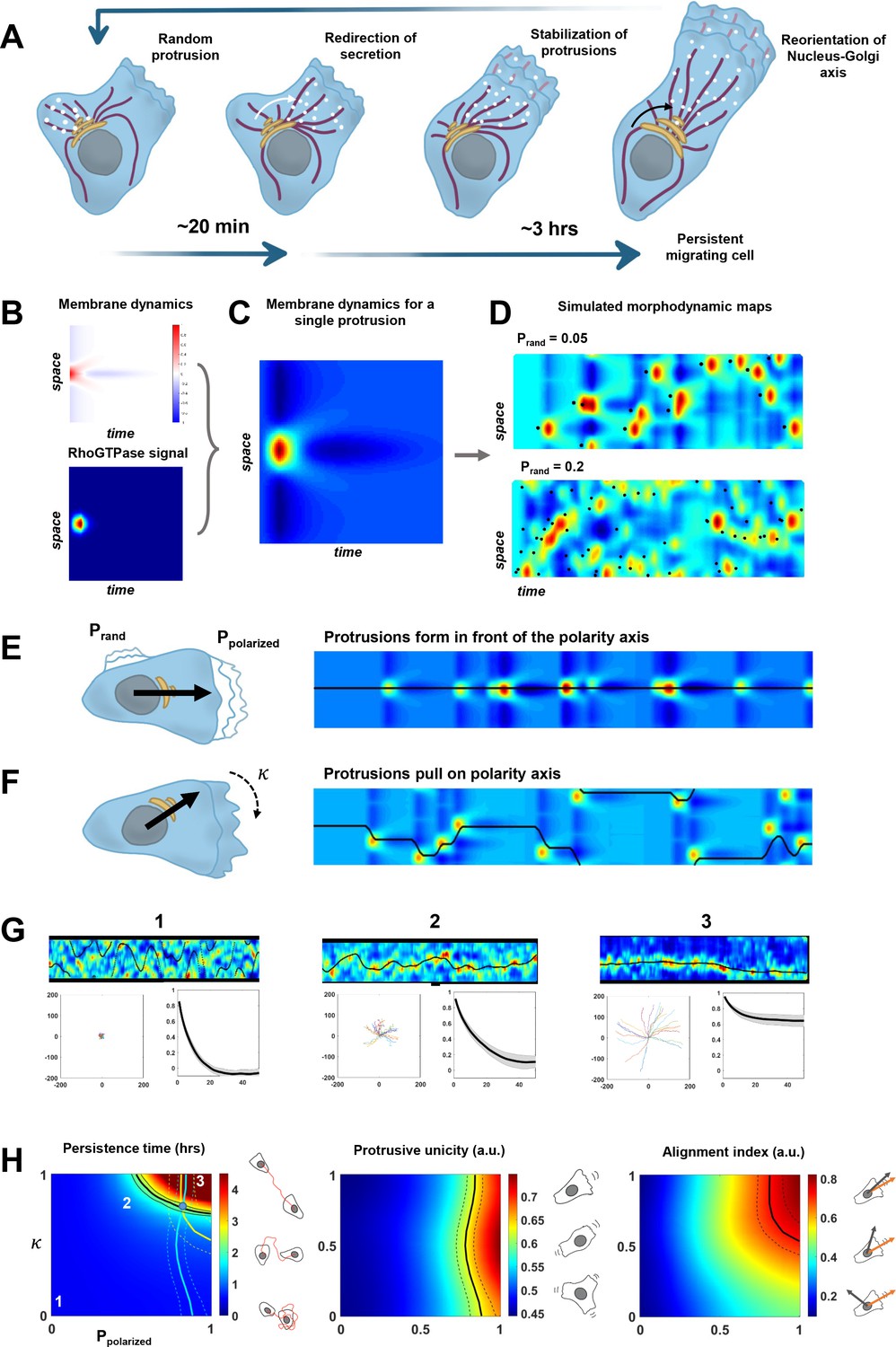
A minimal physical model based on the coupling between protrusive activity and internal polarity recapitulates persistent migration.
(A) Scheme representing the sequence of events leading to persistent migration. The Golgi complex is in yellow, microtubules are in violet, and vesicles in white. (B–C) Membrane dynamics for a point-like Cdc42 activation (A, upper panel) were convolved with a RhoGTPases signal (A, lower panel) to compute membrane dynamics for a single protrusive event (B). (D) Overall synthetic morphodynamic maps generated by varying the protrusive activity frequency. The intensity of protrusive activity varies from one protrusion every 20 frames (top), to one every 5 frames (bottom), the latter value having been retained for our simulations in (G–H). (E–F) Implementation of the feedback, with quantifying the probability to form a protrusion in front of the polarity axis (equal to one in the simulated morphodynamic map in (E)), and quantifying the capacity of protrusions to pull on the polarity axis (equal to one the simulated morphodynamic map in (F)). (G) Examples of morphodynamic maps (top, black line is the direction of the internal polarity axis), cell trajectories (bottom left), and autocorrelation of direction (bottom right) for different values of strength of the feedback. 1: . 2: . 3: . (H) Phase diagrams of persistence time, protrusive unicity, and alignment index. Black lines in the diagrams correspond to the experimental values (persistent time ~2 hr, protrusive unicity ~0.6 and alignment index ~0.7). The lines of the two last diagrams are reported on the first one, where they cross at a single point (blue dot), hereby showing consistency between the model and our experimental measurements. Data used for A-H, related scripts and additional explanations can be found in Figure 6—source data 1.
-
Figure 6—source data 1
Data and analysis scripts with explanations for Figure 6 and its supplements.
- https://cdn.elifesciences.org/articles/69229/elife-69229-fig6-data1-v2.zip
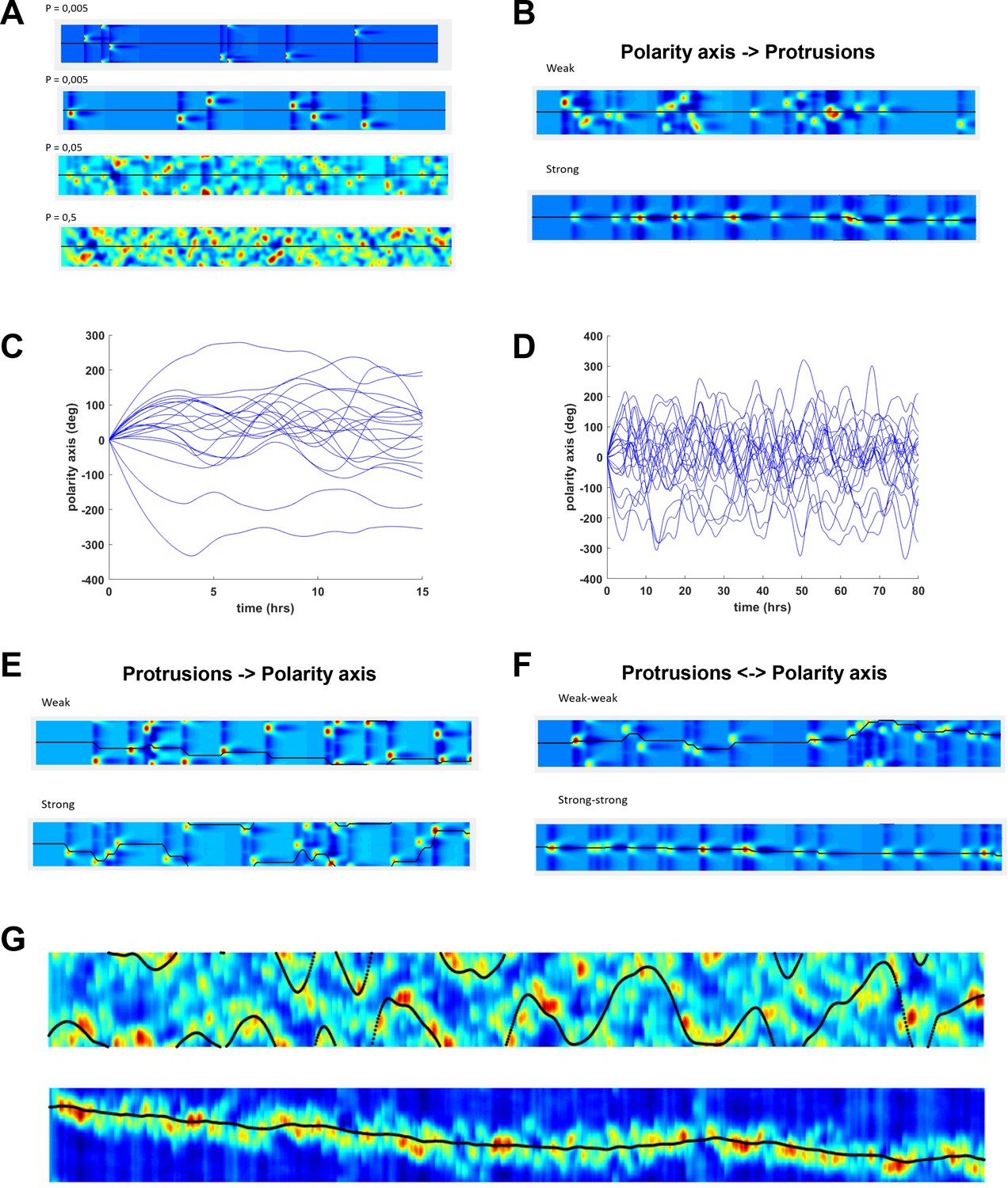
Figure 6—figure supplement 1
Detailed explanation of the minimal physical model.
(A) Example of morphodynamic maps without any feedback for varying frequencies of protrusions. The x-axis is time (1000 frames) and the y-axis is the contour along the cell, . The color code represents membrane speed in arbitrary units, from deep blue (retraction) to deep red (protrusion). (B) Example of morphodynamic maps with two extreme values of the feedback between polarity axis and protrusions. The direction of the polarity axis is depicted by the central black line which corresponds to the position of over time. In the top figure, there is a weak tendency to form protrusions in the direction of the polarity axis. In the bottom figure, there is a strong tendency to form protrusions in the direction of the polarity axis. The x-axis is time (1000 frames) and the y-axis is the contour along the cell, . The color code represents membrane speed in arbitrary units, from deep blue (retraction) to deep red (protrusion). (C–D) Natural evolution of the polarity axis in the simulation for 150 frames (~15 hr) for 20 repetitions (C) and for 1000 frames (~80 hr) for 20 repetitions (D). (E) Example of morphodynamic maps with two extreme values of the feedback between protrusions and polarity axis. The direction of the polarity axis is depicted by the black line which corresponds to the position of over time. In the top figure, there is a weak tendency of the polarity axis to follow protrusions, whereas in the bottom figure, there is a strong tendency of the polarity axis to align with every protrusion. The x-axis is time (1000 frames) and the y-axis is the contour along the cell, . The color code represents membrane speed in arbitrary units, from deep blue (retraction) to deep red (protrusion). (F) Example of morphodynamic maps with the two sides of the feedback in action. The direction of the polarity axis is depicted by the black line, which corresponds to the position of over time. The top figure corresponds to weak feedback, and the bottom figure to strong feedback. The x-axis is time (1000 frames) and the y-axis is the contour along the cell, . The color code represents membrane speed in arbitrary units, from deep blue (retraction) to deep red (protrusion). (G) Example of morphodynamic maps with the two sides of the feedback in action, for realistic frequencies of protrusion per unit of time. The direction of the polarity axis is depicted by the black line which corresponds to the position of over time. The top figure corresponds to intermediate feedback () that still leads to random migration. The bottom figure corresponds to strong feedback () that leads to very persistent migration. The x-axis is time (1000 frames) and the y-axis is the contour along the cell, . The color code represents membrane speed in arbitrary units, from deep blue (retraction) to deep red (protrusion).
Figure 6—figure supplement 2
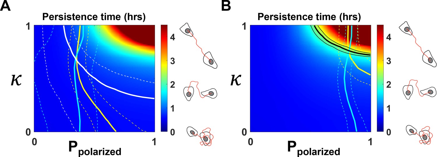
Comparison of phase diagrams of HeLa and RPE1 cells.
(A) Phase diagram of persistence time for HeLa cells. Persistence time is 0.7 ± 0.17 (SEM), white line; protrusive unicity is 0.420.7 ± 0.03 (SEM), cyan line; alignment index is 0.26 ± 0.06 (SEM), yellow line (N = 17). (B) Phase diagram of persistence time for RPE1 cells, as in Figure 6 of the main manuscript shown here for comparison. Data used and related scripts can be found in Figure 6—source data 1.
Figure 6—figure supplement 3
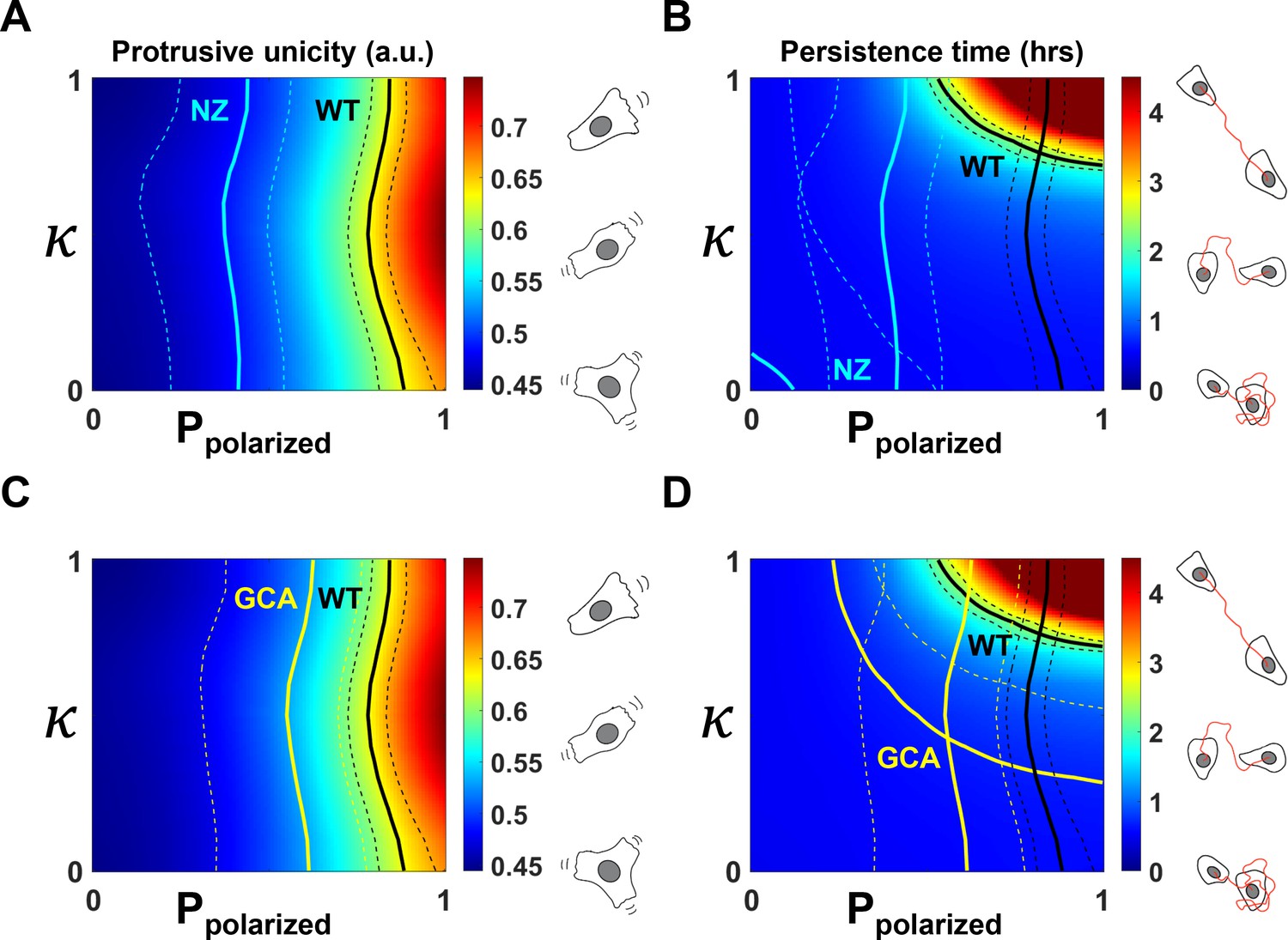
Comparison of phase diagrams of Nocodazole and Golgicide A treated RPE1 cells.
Heat maps of persistence time and protrusive unicity to compare between wild-type (WT) cells and Nocodazole (NZ) treated cells (A–B) and WT cells, and Golgicide A (GCA) treated cells (C–D). Data used and related scripts can be found in Figure 6—source data 1.
Figure 6—video 1
Movement of a synthetic cell recapitulated by the minimal physical model.
Author response image 1
Author response image 2
Tables
Key resources table
| Reagent type (species) or resource | Designation | Source or reference | Identifiers | Additional information |
|---|---|---|---|---|
| Cell line (Homo sapiens) | hTERT RPE1 (immortalized, normal, female) | ATCC | ATCC Cat# CRL-4000, RRID:CVCL_4388 | |
| Cell line (H. sapiens) | HeLa (adenocarcinoma, female) | ATCC | ATCC Cat# CCL-2, RRID:CVCL_0030 | |
| Cell line (H. sapiens) | RPE1::iRFP-Rab6A | This paper | Heterozygous iRFP-Rab6A CRISPR knock-in | |
| Cell line (H. sapiens) | RPE1::iRFP-Rab6::hITSN1-tgRFP-SSPB wtt::Venus-iLID-CAAX | This paper | Stable cell line with heterozygous iRFP-Rab6A label and lentivirally induced expression of optogenetic constructs | |
| Cell line (H. sapiens) | RPE1::GFP-Rab6A | This paper | Lentivirally induced stable GFP-Rab6A overexpression | |
| Cell line (H. sapiens) | RPE1::GFP-Rab6A::myr-iRFP | This paper | Stable cell line with GFP-Rab6A and myr-iRFP overexpression | |
| Cell line (H. sapiens) | RPE1::EGFP-α-tubulin | Piel lab | Stable cell line with a α-tubulin marker | |
| Cell line (H. sapiens) | RPE1::EB3-EGFP | https://doi.org/10.1038/nmeth.1493 | Krek lab | |
| Transfected construct (H. sapiens) | pLL7.0: hITSN1(1159–1509)-tgRFPt-SSPB WT | Addgene | RRID: Addgene_60419 | Lentiviral optogenetic construct for Cdc42 activation |
| Transfected construct (H. sapiens) | pLL7.0: Venus-iLID-CAAX | Addgene | RRID: Addgene_60411 | Lentiviral optogenetic construct |
| Transfected construct (H. sapiens) | pMD2.G | Addgene | RRID: Addgene_12259 | Lentiviral VSV-G envelope expressing plasmid |
| Transfected construct (H. sapiens) | psPAX2 | Addgene | RRID:Addgene_12260 | Second generation lentiviral packaging plasmid |
| Transfected construct (H. sapiens) | pHR: myr-iRFP | Coppey lab | Lentiviral construct to label plasma membrane with iRFP | |
| Transfected construct (H. sapiens) | pEGFP-C3: Rab6A_wt | Goud lab | Plasmid construct to label Rab6A (Golgi complex) | |
| Transfected construct (H. sapiens) | pIRESneo3: Str-KDEL-SBP-EGFP-COL10A1 | https://doi.org/10.1083/jcb.201805002 | RUSH system plasmid with EGFP tagged Collagen X cargo | |
| Antibody | anti-GFP (rabbit monoclonal) | Recombinant Antibody Platform of Institut Curie | Cat#:A-P-R#06 | (dilution 1:100) |
| Antibody | anti-α-Tubulin (mouse monoclonal) | Sigma Aldrich | Sigma-Aldrich Cat# T5168, RRID:AB_477579 | (dilution 1:1000) |
| Antibody | Anti-mouse AlexaFluor 546 F(ab’)2 fragment of IgG (H + L) (goat polyclonal) | Life Technologies | (dilution 1:1000) | |
| Sequence-based reagent | gRNA-3-mRAB6A | Eurofins | sgRNA | GTCTCCGCCCGTGGACATTG |
| Chemical compound, drug | Nocodazole | Sigma Aldrich | M1404 | (0.1 µM) |
| Chemical compound, drug | Golgicide A | Sigma Aldrich | G0923 | (35 µM) |
| Chemical compound, drug | Taxol | Sigma Aldrich | T7402 | (0.1 µM) |
| Chemical compound, drug | Biotin | Sigma Aldrich | B4501 | (40 µM) |
| Chemical compound, drug | Poly-L-lysine | Sigma Aldrich | P8920 | (0.01% diluted in water) |
| Chemical compound, drug | Fibronectin | Sigma Aldrich | F1141 | (2 µg/mL; 10 µg/mL; 20 µg/mL) |
| Chemical compound, drug | PLL-g-PEG | Surface Solutions | PLL(20)-g[3.5]- PEG(2) | (100 µg/mL) |
| Chemical compound, drug | azido-PLL-g-PEG (APP) | https://doi.org/10.1002/adma.201204474 | (100 µg/mL) | |
| Chemical compound, drug | BCN-RGD | https://doi.org/10.1002/adma.201204474 | (20 µM) | |
| Software, algorithm | Matlab | MathWorks | RRID:SCR_001622 | |
| Software, algorithm | Fiji, ImageJ | https://doi.org/10.1038/nmeth.2019 | RRID:SCR_002285 | |
| Software, algorithm | Trackmate | https://doi.org/10.1016/j.ymeth.2016.09.016https://doi.org/10.1016/j.ymeth.2016.09.016 | ||
| Software, algorithm | MetaMorph | Molecular Devices | RRID:SCR_002368 | |
| Other | Hoechst 33,342 | Thermo Fisher Scientific | H3570 | (1 µg/mL) |
| Other | DAPI stain | Merck | D9542 | (1 µg/mL) |
Additional files
Download links
A two-part list of links to download the article, or parts of the article, in various formats.
Downloads (link to download the article as PDF)
Open citations (links to open the citations from this article in various online reference manager services)
Cite this article (links to download the citations from this article in formats compatible with various reference manager tools)
Persistent cell migration emerges from a coupling between protrusion dynamics and polarized trafficking
eLife 11:e69229.
https://doi.org/10.7554/eLife.69229


