Tracking cell lineages in 3D by incremental deep learning
- Institut de Génomique Fonctionnelle de Lyon (IGFL), École Normale Supérieure de Lyon, France
- Centre National de la Recherche Scientifique (CNRS), France
Figures
Figure 1 with 2 supplements
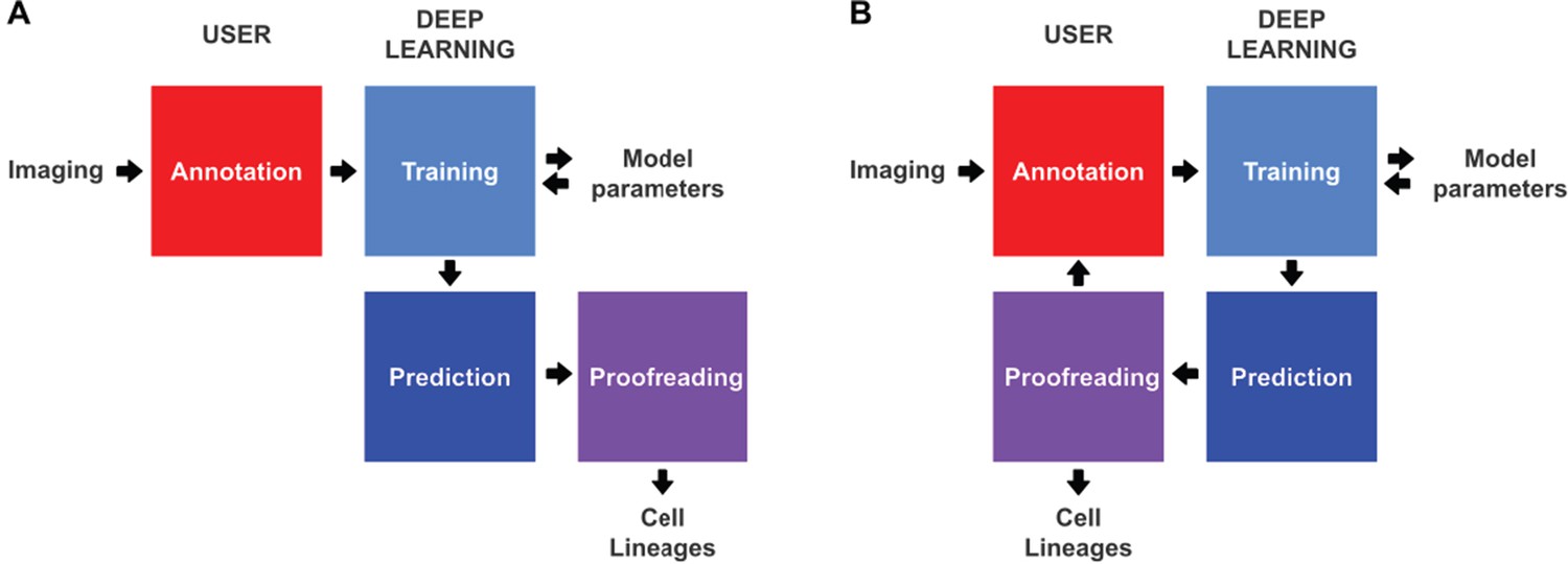
Conventional and incremental deep learning workflows for cell tracking.
(A) Schematic illustration of a typical deep learning workflow, starting with the annotation of imaging data to generate training datasets, training of deep learning models, prediction by deep learning and proofreading. (B) Schematic illustration of incremental learning with ELEPHANT. Imaging data are fed into a cycle of annotation, training, prediction, and proofreading to generate cell lineages. At each iteration, model parameters are updated and saved. This workflow applies to both detection and linking phases (see Figures 2A and 4A).
Figure 1—figure supplement 1
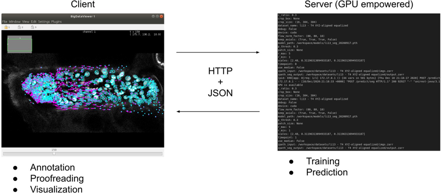
ELEPHANT client-server architecture.
The client provides an interactive user interface for annotation, proofreading, and visualization. The server performs training and prediction with deep learning. The client and server communicate using HTTP and JSON.
Figure 1—figure supplement 2
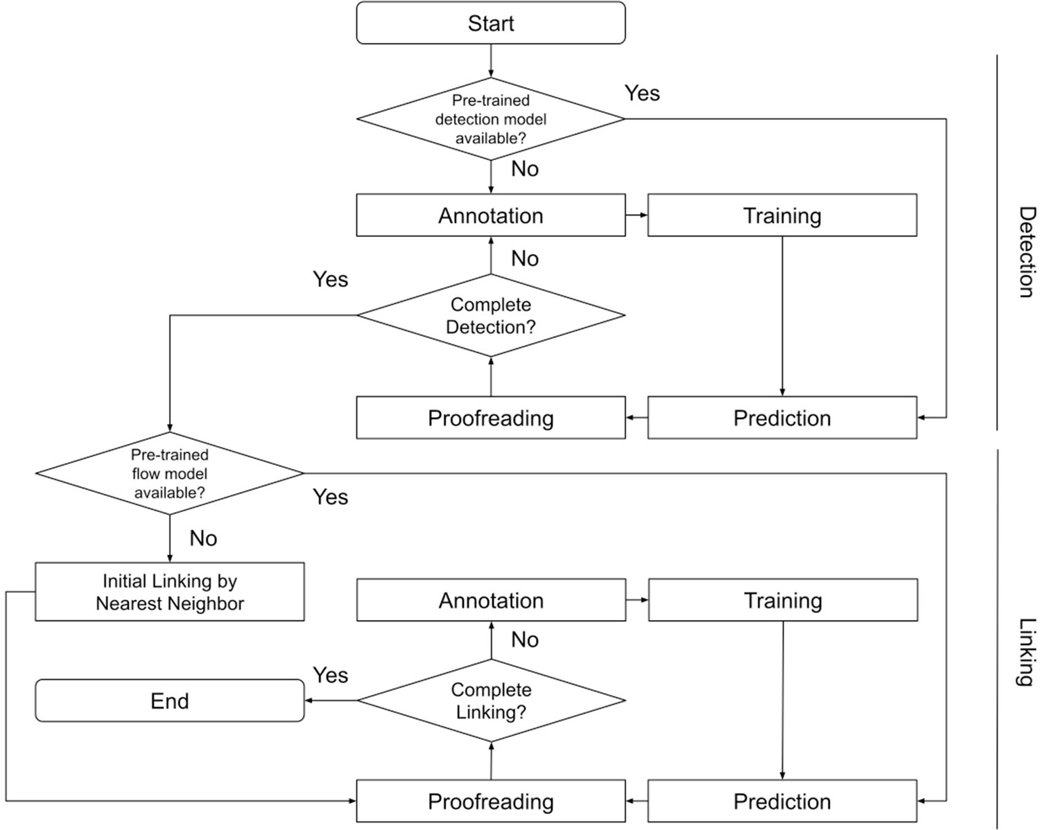
Block diagram of ELEPHANT tracking workflow.
A block diagram showing how the entire tracking workflow can be performed using ELEPHANT.
Figure 2 with 2 supplements
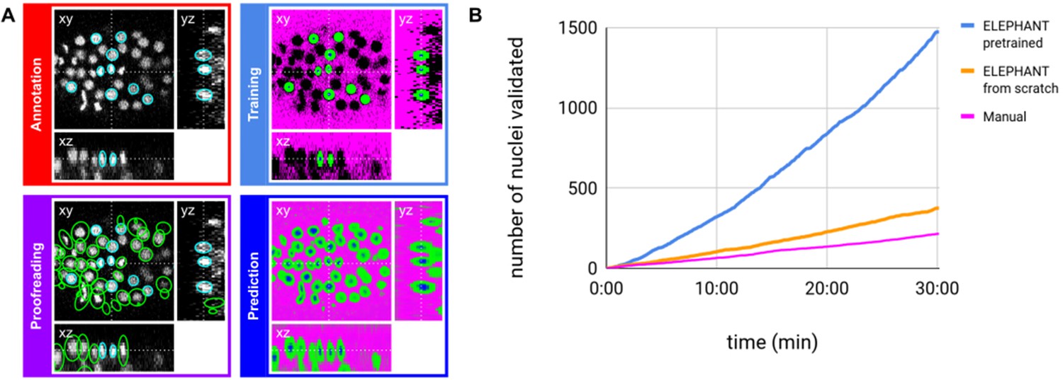
ELEPHANT detection workflow.
(A) Detection workflow, illustrated with orthogonal views on the CE1 dataset. Top left: The user annotates nuclei with ellipsoids in 3D; newly generated annotations are colored in cyan. Top right: The detection model is trained with the labels generated from the sparse annotations of nuclei and from the annotation of background (in this case by intensity thresholding); background, nucleus center, nucleus periphery and unlabelled voxels are indicated in magenta, blue, green, and black, respectively. Bottom right: The trained model generates voxel-wise probability maps for background (magenta), nucleus center (blue), or nucleus periphery (green). Bottom left: The user validates or rejects the predictions; predicted nuclei are shown in green, predicted and validated nuclei in cyan. (B) Comparison of the speed of detection and validation of nuclei on successive timepoints in the CE1 dataset, by manual annotation (magenta), semi-automated detection without a pre-trained model (orange) and semi-automated detection using a pre-trained model (blue) using ELEPHANT.
Figure 2—figure supplement 1
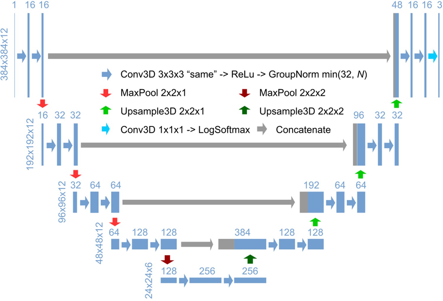
3D U-Net architecture for detection.
Schematic illustration of the 3D U-Net architecture for detection, using an input image with a size of 384 × 384 x 12 and a ratio of lateral-to-axial resolution of 8 as an example. Rectangles show the input/intermediate/output layers, with the sizes shown on the left of each row and the number of channels shown above each rectangle. Block arrows represent different operations as described in the figure. The resolution of the z dimension is maintained until the image becomes nearly isotropic (ratio of lateral-to-axial resolution of 1, in the bottom layers in this example).
Figure 2—figure supplement 2
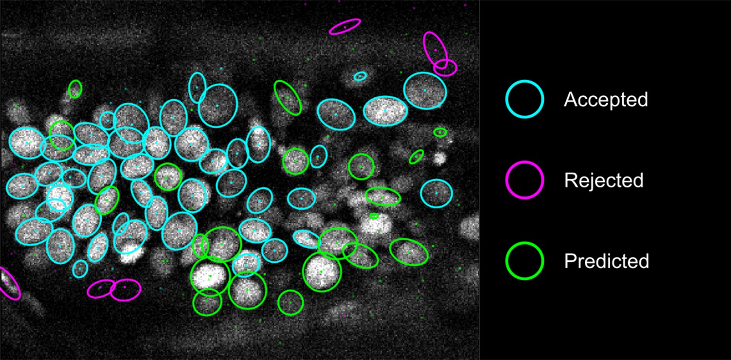
Proofreading in detection.
The ellipses show the sections of nuclear annotations in the xy plane and the dots represent the projections of the center position of the annotated nuclei, drawn in distinct colors; color code explained on the right. Nuclei that are out of focus in this view appear only as dots.
Figure 3 with 2 supplements
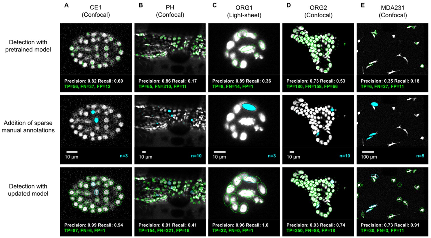
ELEPHANT detection with sparse annotations.
Detection results obtained using ELEPHANT with sparse annotations on five image datasets recording the embryonic development of C. elegans (CE1 dataset, A), leg regeneration in the crustacean P. hawaiensis (PH dataset, B), human intestinal organoids (ORG1 and ORG2, C and D), and human breast carcinoma cells (MDA231, E). CE1, PH, ORG2, and MDA231 were captured by confocal microscopy; ORG1 was captured by light sheet microscopy. Top: Detection results using models that were pre-trained on diverse annotated datasets, excluding the test dataset (see Supplementary file 3). Precision and Recall scores are shown at the bottom of each panel, with the number of true positive (TP), false positive (FP), and false negative (FN) predicted nuclei. Middle: Addition of sparse manual annotations for each dataset. n: number of sparse annotations. Scale bars: 10 µm. Bottom: Detection results with an updated model that used the sparse annotations to update the pre-trained model. Precision, Recall, TP, FP, and FN values are shown as in the top panels.
Figure 3—figure supplement 1
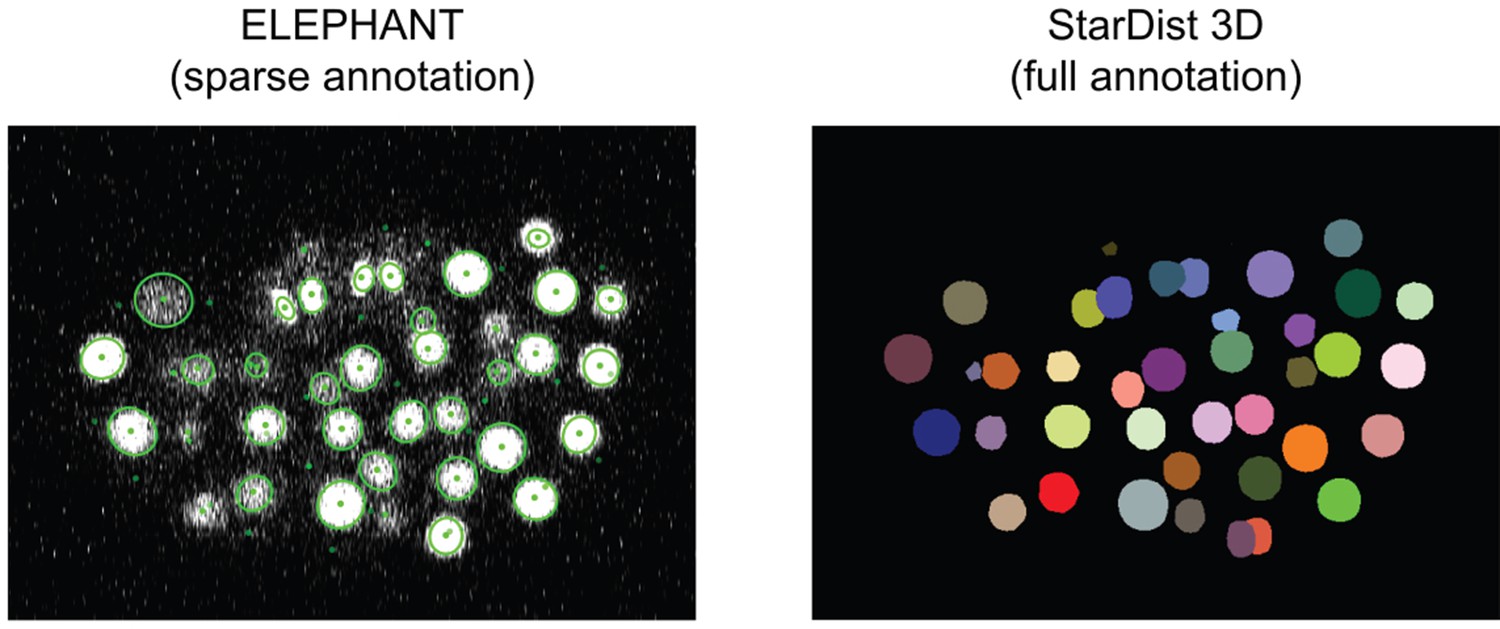
Comparing detection predictions of ELEPHANT and StarDist3D.
ELEPHANT and StarDist3D models were trained with the CE1 dataset (timepoint = 100) and tested on the CE2 dataset (timepoint = 100). The ELEPHANT model was trained from scratch with sparse annotations (10 nuclei, as shown in Figure 3—figure supplement 2), whereas the StarDist3D model was trained with full annotations (93 nuclei). The cell instances segmented by StarDist3D are color-coded in Fiji. The DET scores were 0.975 (ELEPHANT) and 0.999 (StarDist3D), respectively.
Figure 3—figure supplement 2
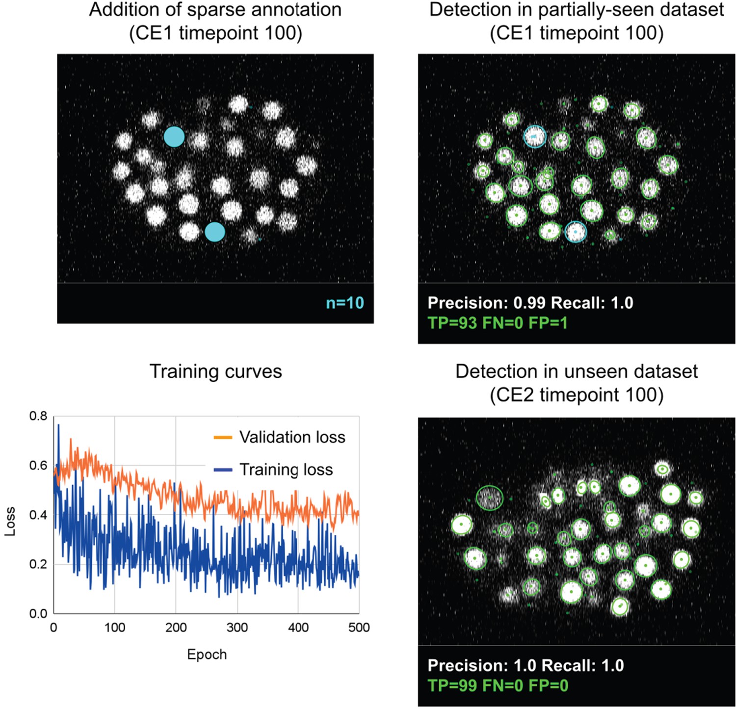
Evaluation of overfitting in detection using ELEPHANT.
An ELEPHANT detection model was trained with 10 sparse annotations for 500 training epochs starting from scratch. The top left panel shows a slice of image volume used for training, on which the sparse annotations are overlaid in cyan. The bottom left plot shows the loss curves in training and validation datasets. The top right and bottom right panels show the detection results on the CE1 (top) and CE2 (bottom) datasets, obtained using the model trained for 500 epochs, where the annotations and predictions are indicated with outlines in cyan and green colors. Precision and Recall scores are shown at the bottom of each panel, with the number of true positive (TP), false positive (FP), and false negative (FN) predicted nuclei.
Figure 4 with 2 supplements

ELEPHANT linking workflow.
(A) Linking workflow, illustrated on the CE1 dataset. Top left: The user annotates links by connecting detected nuclei in successive timepoints; annotated/validated nuclei and links are shown in cyan, non-validated ones in green. Top right: The flow model is trained with optical flow labels coming from annotated nuclei with links (voxels indicated in the label mask), which consist of displacements in X, Y, and Z; greyscale values indicate displacements along a given axis, annotated nuclei with link labels are outlined in red. Bottom right: The trained model generates voxel-wise flow maps for each axis; greyscale values indicate displacements, annotated nuclei are outlined in red. Bottom left: The user validates or rejects the predictions; predicted links are shown in green, predicted and validated links in cyan. (B) Tracking results obtained with ELEPHANT. Left panels: Tracked nuclei in the CE1 and CE2 datasets at timepoints 194 and 189, respectively. Representative optical sections are shown with tracked nuclei shown in green; out of focus nuclei are shown as green spots. Right panels: Corresponding lineage trees. (C) Comparison of tracking results obtained on the PH dataset, using the nearest neighbor algorithm (NN) with and without optical flow prediction (left panels); linking errors are highlighted in red on the correct lineage tree. The panels on the right focus on the nuclear division that is marked by a dashed line rectangle. Without optical flow prediction, the dividing nuclei (in magenta) are linked incorrectly.
Figure 4—figure supplement 1
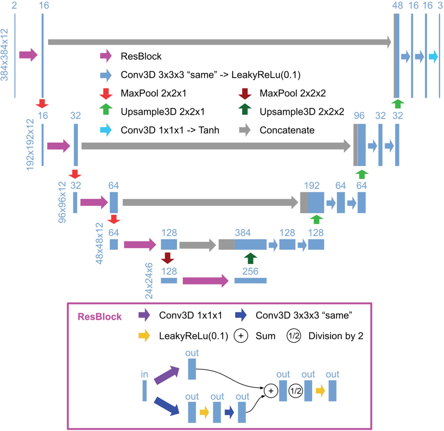
3D U-Net architecture for flow.
Schematic illustration of the 3D U-Net architecture for the flow model, depicted as in Figure 2—figure supplement 1. The structure of ResBlock is shown on the bottom.
Figure 4—video 1
ELEPHANT flow predictions in 3D.
The PH dataset is shown in parallel with the corresponding flow predictions of the ELEPHANT optical flow model (in three dimensions), over the entire duration of the recording. Gray values for flow predictions represent displacements between timepoints as introduced in Figure 4A.
Figure 5 with 3 supplements
Cell lineages tracked during the time course of leg regeneration.
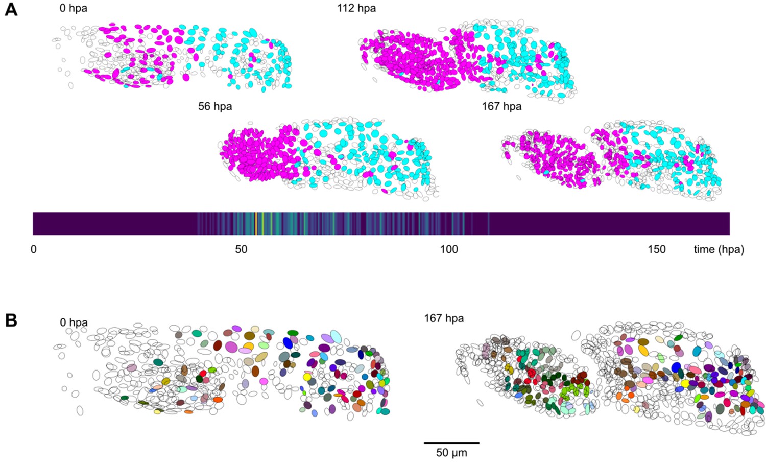
(A) Spatial and temporal distribution of dividing nuclei in the regenerating leg of Parhyale tracked over a 1-week time course (PH dataset), showing that cell proliferation is concentrated at the distal part of the regenerating leg stump and peaks after a period of proliferative quiescence, as described in Alwes et al., 2016. Top: Nuclei in lineages that contain at least one division are colored in magenta, nuclei in non-dividing lineages are in cyan, and nuclei in which the division status is undetermined are blank (see Materials and methods). Bottom: Heat map of the temporal distribution of nuclear divisions; hpa, hours post amputation. The number of divisions per 20-min time interval ranges from 0 (purple) to 9 (yellow). (B) Fate map of the regenerating leg of Parhyale, encompassing 109 fully tracked lineage trees (202 cells at 167 hpa). Each clone is assigned a unique color and contains 1–9 cells at 167 hpa. Partly tracked nuclei are blank. In both panels, the amputation plane (distal end of the limb) is located on the left.
Figure 5—figure supplement 1
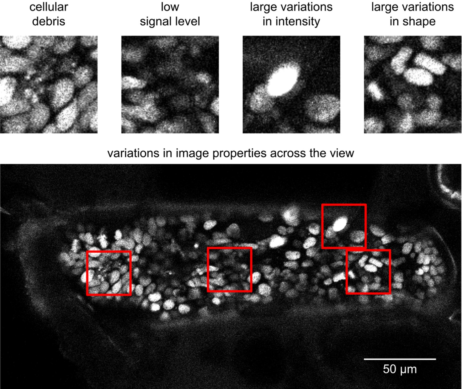
Image quality issues in the PH dataset.
Snapshots represent the image characteristics of the PH dataset that render cell tracking more challenging: fluorescence from cellular debris, low signal, variations in nuclear fluorescence intensity and nuclear shape, and variations in image quality across the imaged sample. The top panels show parts of a field of view indicated with red squares; the bottom panel shows an entire xy plane.
Figure 5—figure supplement 2
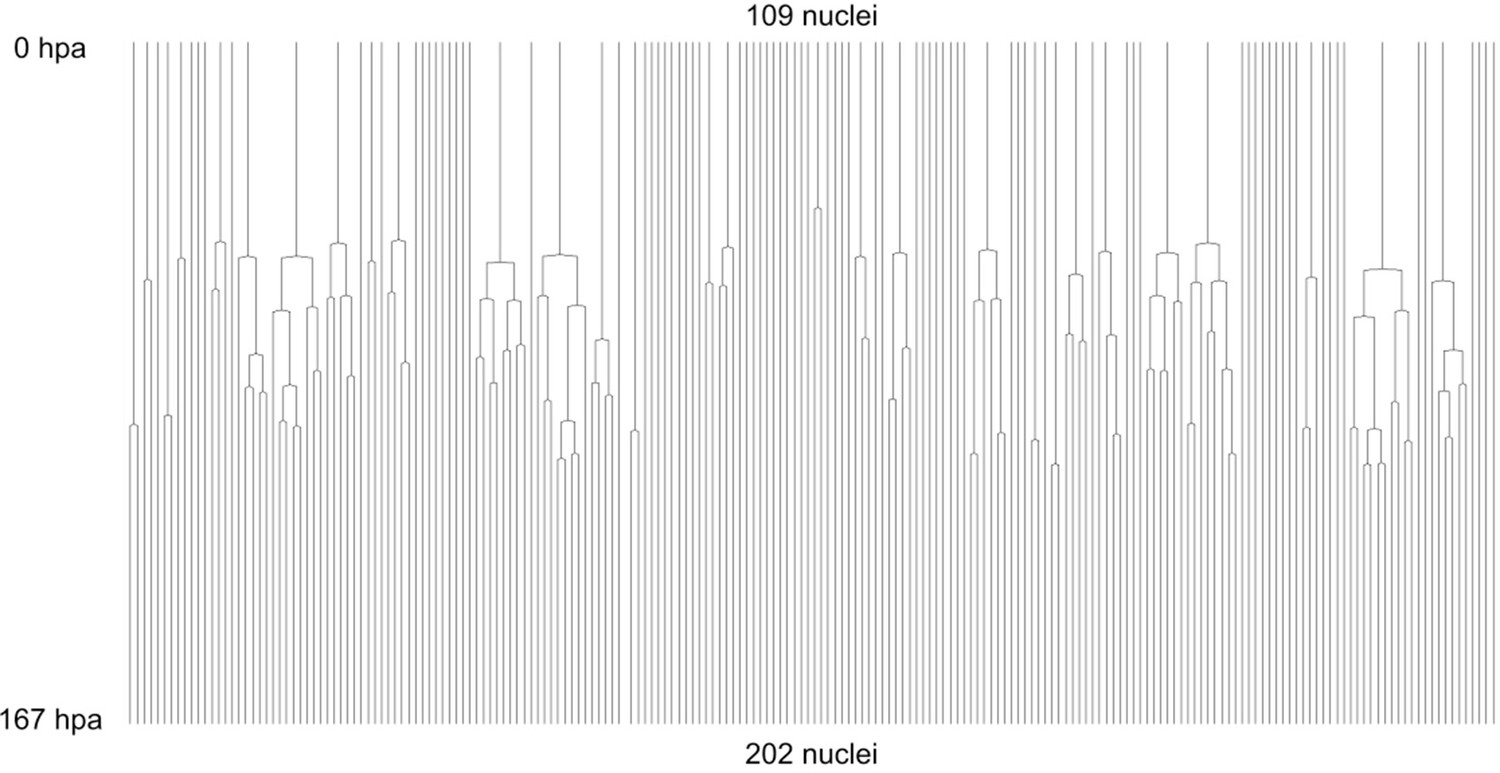
Complete cell lineage trees in a regenerating leg of Parhyale.
The displayed trees contain 109 complete and fully validated cell lineages in a regenerating leg of Parhyale (PH dataset), corresponding to Figure 5.
Figure 5—video 1
Live imaging of Parhyale leg regeneration (PH dataset).
A maximum intensity projection of the PH dataset captures the regeneration of a Parhyale T4 leg amputated at the distal end of the carpus, over a period of 1 week. hpa, hours post amputation.
Tables
Table 1
Performance of ELEPHANT on the Cell Tracking Challenge dataset.
Performance of ELEPHANT compared with two state-of-the-art algorithms, using the metrics of the Cell Tracking Challenge on unseen CE datasets. ELEPHANT outperforms the other methods in detection and linking accuracy (DET and TRA metrics); it performs less well in segmentation accuracy (SEG).
| ELEPHANT | KTH-SE | KIT-Sch-GE | |
|---|---|---|---|
| (IGFL-FR) | |||
| SEG | 0.631 | 0.662 | 0.729 |
| TRA | 0.975 | 0.945 | 0.886 |
| DET | 0.979 | 0.959 | 0.930 |
Additional files
-
Supplementary file 1
Processing speed of the detection model Processing speed of the deep learning model for the detection of nuclei, applied to three datasets.
The training speed is affected by the distribution of annotations because the algorithm contains a try-and-error process for cropping, in which the nucleus periphery labels are forced to appear with the nucleus center labels.
- https://cdn.elifesciences.org/articles/69380/elife-69380-supp1-v1.xlsx
-
Supplementary file 2
Comparison of linking performances Linking performances on the PH dataset, on a total number of 259,071 links (including 688 links on cell divisions).
Incremental training was performed by transferring the training parameters from the model pre-trained with the CE datasets. Linking performance on dividing cells is scored separately.
- https://cdn.elifesciences.org/articles/69380/elife-69380-supp2-v1.xlsx
-
Supplementary file 3
Datasets used for training generic detection models Datasets used in training of the detection models used in Figure 3.
Columns correspond to the datasets analysed in Figure 3 and rows indicate the image datasets included in the training. In each case, the test image data were excluded from training. The Fluo-C3DH-A549 (Castilla et al., 2019), Fluo-C3DH-H157 (Maška et al., 2013), Fluo-N3DH-CHO (Dzyubachyk et al., 2010), Fluo-N3DH-CE (Murray et al., 2008) datasets are from the Cell Tracking Challenge (Maška et al., 2014).
- https://cdn.elifesciences.org/articles/69380/elife-69380-supp3-v1.xlsx
-
Supplementary file 4
Parameters used for training and prediction using StarDist3D Parameters used for training and prediction in the StarDist3D model used in Figure 3—figure supplement 1.
These parameters were extracted from “config.json” and “thresholds.json” generated by the software.
- https://cdn.elifesciences.org/articles/69380/elife-69380-supp4-v1.xlsx
-
Supplementary file 5
Parameters used for training and validation of generic models Parameters used for training and validation of the generic models used in Figure 3.
Size and scale are represented in the format [X]x[Y]x[Z].
- https://cdn.elifesciences.org/articles/69380/elife-69380-supp5-v1.xlsx
-
Supplementary file 6
Parameters used for fine-tuning and prediction using generic models Parameters used for fine-tuning of the generic models and prediction used in Figure 3.
Size and scale are represented in the format [X]x[Y]x[Z].
- https://cdn.elifesciences.org/articles/69380/elife-69380-supp6-v1.xlsx
-
Transparent reporting form
- https://cdn.elifesciences.org/articles/69380/elife-69380-transrepform1-v1.docx
Download links
A two-part list of links to download the article, or parts of the article, in various formats.
Downloads (link to download the article as PDF)
Open citations (links to open the citations from this article in various online reference manager services)
Cite this article (links to download the citations from this article in formats compatible with various reference manager tools)
Tracking cell lineages in 3D by incremental deep learning
eLife 11:e69380.
https://doi.org/10.7554/eLife.69380


