Tracking cell lineages in 3D by incremental deep learning

Version of Record

Accepted for publication after peer review and revision.

Download
Cite
Share
CommentOpen annotations (there are currently 0 annotations on this page).

Version of Record published: January 6, 2022 (This version)
Accepted: December 7, 2021
Received: April 13, 2021
Preprint posted: February 26, 2021 (Go to version)

1. Of interest
Transcription: A hub of activity

Virginia L Pimmett, Mounia Lagha

Insight Nov 29, 2023
Further reading

Abstract
Introduction
Results and discussion
Materials and methods
Data availability
References
Decision letter
Author response
Article and author information
Metrics

Abstract

Deep learning is emerging as a powerful approach for bioimage analysis. Its use in cell tracking is limited by the scarcity of annotated data for the training of deep-learning models. Moreover, annotation, training, prediction, and proofreading currently lack a unified user interface. We present ELEPHANT, an interactive platform for 3D cell tracking that addresses these challenges by taking an incremental approach to deep learning. ELEPHANT provides an interface that seamlessly integrates cell track annotation, deep learning, prediction, and proofreading. This enables users to implement cycles of incremental learning starting from a few annotated nuclei. Successive prediction-validation cycles enrich the training data, leading to rapid improvements in tracking performance. We test the software’s performance against state-of-the-art methods and track lineages spanning the entire course of leg regeneration in a crustacean over 1 week (504 timepoints). ELEPHANT yields accurate, fully-validated cell lineages with a modest investment in time and effort.

Introduction

Recent progress in deep learning has led to significant advances in bioimage analysis (Moen et al., 2019; Ouyang et al., 2018; Weigert et al., 2018). As deep learning is data-driven, it is adaptable to a variety of datasets once an appropriate model architecture is selected and trained with adequate data (Moen et al., 2019). In spite of its powerful performance, deep learning remains challenging for non-experts to utilize, for three reasons. First, pre-trained models can be inadequate for new tasks and the preparation of new training data is laborious. Because the quality and quantity of the training data are crucial for the performance of deep learning, users must invest significant time and effort in annotation at the start of the project (Moen et al., 2019). Second, an interactive user interface for deep learning, especially in the context of cell tracking, is lacking (Kok et al., 2020; Wen et al., 2021). Third, deep learning applications are often limited by accessibility to computing power (high-end GPU).

We have addressed these challenges by establishing ELEPHANT (Efficient learning using sparse human annotations for nuclear tracking), an interactive web-friendly platform for cell tracking, which seamlessly integrates manual annotation with deep learning and proofreading of the results. ELEPHANT implements two algorithms optimized for incremental deep learning using sparse annotations, one for detecting nuclei in 3D and a second for linking these nuclei across timepoints in 4D image datasets. Incremental learning allows models to be trained in a stepwise fashion on a given dataset, starting from sparse annotations that are incrementally enriched by human proofreading, leading to a rapid increase in performance (Figure 1). ELEPHANT is implemented as an extension of Mastodon (https://github.com/mastodon-sc/mastodon; Mastodon Science, 2021), an open-source framework for large-scale tracking deployed in Fiji (Schindelin et al., 2012). It implements a client-server architecture, in which the server provides a deep learning environment equipped with sufficient GPU (Figure 1—figure supplement 1).

Figure 1 with 2 supplements see all

Download asset Open asset

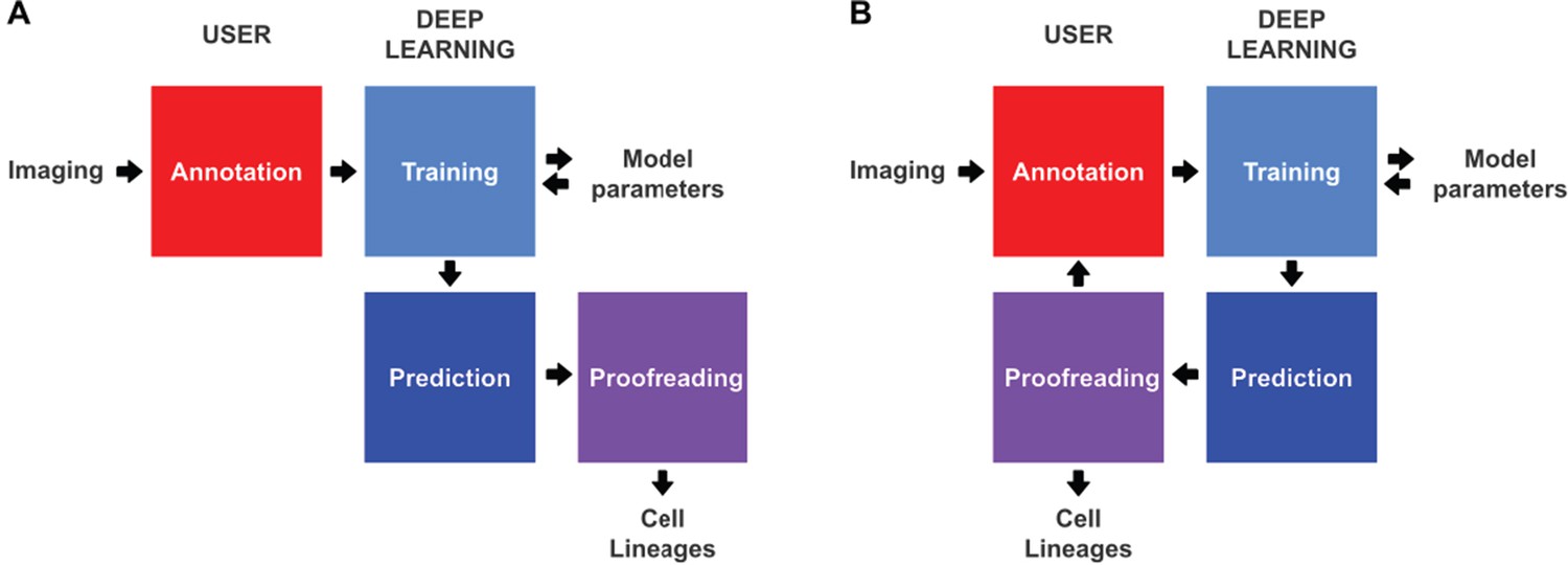
Conventional and incremental deep learning workflows for cell tracking.

(A) Schematic illustration of a typical deep learning workflow, starting with the annotation of imaging data to generate training datasets, training of deep learning models, prediction by deep learning and proofreading. (B) Schematic illustration of incremental learning with ELEPHANT. Imaging data are fed into a cycle of annotation, training, prediction, and proofreading to generate cell lineages. At each iteration, model parameters are updated and saved. This workflow applies to both detection and linking phases (see Figures 2A and 4A).

Results and discussion

ELEPHANT employs the tracking-by-detection paradigm (Maška et al., 2014), which involves initially the detection of nuclei in 3D and subsequently their linking over successive timepoints to generate tracks. In both steps, the nuclei are represented as ellipsoids, using the data model of Mastodon (Figure 2A and Figure 4A). We use ellipsoids for annotation because ellipsoids allow rapid and efficient training and prediction, compared with more complex shapes. This is essential for interactive deep learning. In the detection phase, voxels are labelled as background, nucleus center or nucleus periphery, or left unlabelled (Figure 2A, top right). The nucleus center and nucleus periphery labels are generated by the annotation of nuclei, and the background can be annotated either manually or by intensity thresholding. Sparse annotations (e.g. of a few nuclei in a single timepoint) are sufficient to start training. A U-Net convolutional neural network (U-Net CNN; Cicek et al., 2016; Ronneberger et al., 2015, Figure 2—figure supplement 1) is then trained on these labels (ignoring the unlabelled voxels) to generate voxel-wise probability maps for background, nucleus center, or nucleus periphery, across the entire image dataset (Figure 2A, bottom right). Post-processing on these probability maps yields predictions of nuclei which are available for visual inspection and proofreading (validation or rejection of each predicted nucleus) by the user (Figure 2A, bottom left). Human-computer interaction is facilitated by color coding of the annotated nuclei as predicted (green), accepted (cyan), or rejected (magenta) (see Figure 2—figure supplement 2), based on the proofreading. The cycles of training and prediction are rapid because only a small amount of training data are added each time (in the order of seconds, see Supplementary file 1). As a result, users can enrich the annotations by proofreading the output almost simultaneously, enabling incremental training of the model in an efficient manner.

Figure 2 with 2 supplements see all

Download asset Open asset

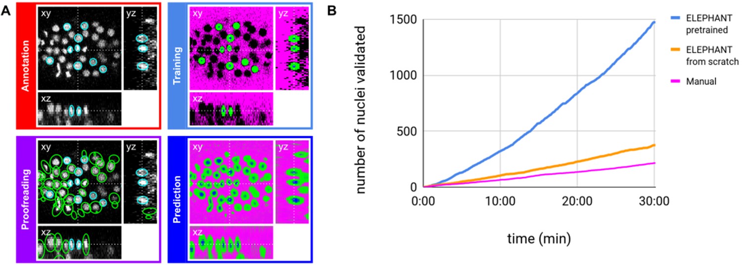
ELEPHANT detection workflow.

(A) Detection workflow, illustrated with orthogonal views on the CE1 dataset. Top left: The user annotates nuclei with ellipsoids in 3D; newly generated annotations are colored in cyan. Top right: The detection model is trained with the labels generated from the sparse annotations of nuclei and from the annotation of *background* (in this case by intensity thresholding); *background*, *nucleus center*, *nucleus periphery* and unlabelled voxels are indicated in magenta, blue, green, and black, respectively. Bottom right: The trained model generates voxel-wise probability maps for *background* (magenta), *nucleus center* (blue), or *nucleus periphery* (green). Bottom left: The user validates or rejects the predictions; predicted nuclei are shown in green, predicted and validated nuclei in cyan. (B) Comparison of the speed of detection and validation of nuclei on successive timepoints in the CE1 dataset, by manual annotation (magenta), semi-automated detection without a pre-trained model (orange) and semi-automated detection using a pre-trained model (blue) using ELEPHANT.

We evaluated the detection performance of ELEPHANT on diverse image datasets capturing the embryonic development of Caenorhabditis elegans (CE1), leg regeneration in the crustacean Parhyale hawaiensis (PH), human intestinal organoids (ORG1 and ORG2) and human breast carcinoma cells (MDA231) by confocal or light sheet microscopy (Figure 3A–E). First, we tested the performance of a generic model that had been pre-trained with various annotated image datasets (Figure 3A–E top). We then annotated 3–10 additional nuclei or cells on each test dataset (Figure 3A–E middle) and re-trained the model. This resulted in greatly improved detection performance (Figure 3A–E), showing that a very modest amount of additional training on a given dataset can yield rapid improvements in performance. We find that sparsely trained ELEPHANT detection models have a comparable performance to state-of-the-art software (Figure 3—figure supplement 1) and fully trained ELEPHANT models outperform most tracking software (Table 1).

Figure 3 with 2 supplements see all

Download asset Open asset

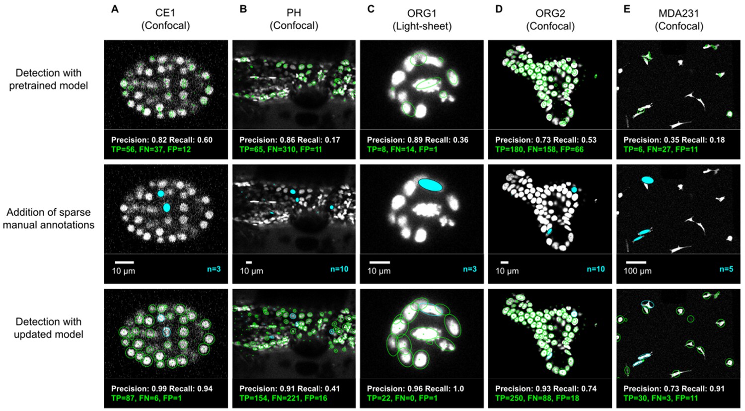
ELEPHANT detection with sparse annotations.

Detection results obtained using ELEPHANT with sparse annotations on five image datasets recording the embryonic development of C. *elegans* (CE1 dataset, A), leg regeneration in the crustacean *P. hawaiensis* (PH dataset, B), human intestinal organoids (ORG1 and ORG2, **C and D**), and human breast carcinoma cells (MDA231, E). CE1, PH, ORG2, and MDA231 were captured by confocal microscopy; ORG1 was captured by light sheet microscopy. Top: Detection results using models that were pre-trained on diverse annotated datasets, excluding the test dataset (see Supplementary file 3). Precision and Recall scores are shown at the bottom of each panel, with the number of true positive (TP), false positive (FP), and false negative (FN) predicted nuclei. Middle: Addition of sparse manual annotations for each dataset. n: number of sparse annotations. Scale bars: 10 µm. Bottom: Detection results with an updated model that used the sparse annotations to update the pre-trained model. Precision, Recall, TP, FP, and FN values are shown as in the top panels.

Table 1

Performance of ELEPHANT on the Cell Tracking Challenge dataset.

Performance of ELEPHANT compared with two state-of-the-art algorithms, using the metrics of the Cell Tracking Challenge on unseen CE datasets. ELEPHANT outperforms the other methods in detection and linking accuracy (DET and TRA metrics); it performs less well in segmentation accuracy (SEG).

	ELEPHANT	KTH-SE	KIT-Sch-GE
	(IGFL-FR)
SEG	0.631	0.662	0.729
TRA	0.975	0.945	0.886
DET	0.979	0.959	0.930

We also investigated whether training with sparse annotations could cause overfitting of the data in the detection model, by training the detection model using sparse annotations in dataset CE1 and calculating the loss values using a second, unseen but similar dataset (see Materials and methods). The training and validation learning curves did not show any signs of overfitting even after a large amount of training (Figure 3—figure supplement 2). The trained model could detect nuclei with high precision and recall both on partially seen data (CE1) and unseen data (CE2). A detection model that has been pre-trained with diverse image datasets is available to users as a starting point for tracking on new image data (see Materials and methods).

In the linking phase, we found that nearest neighbor approaches for tracking nuclei over time (Crocker and Grier, 1996) perform poorly in challenging datasets when the cells are dividing; hence we turned to optical flow modeling to improve linking (Amat et al., 2013; Horn and Schunck, 1981; Lucas and Kanade, 1981). A second U-Net CNN, optimized for optical flow estimation (Figure 4—figure supplement 1), is trained on manually generated/validated links between nuclei in successive timepoints (Figure 4A, top left). Unlabelled voxels are ignored, hence training can be performed on sparse linking annotations. The flow model is used to generate voxel-wise 3D flow maps, representing predicted x, y and z displacements over time (Figure 4A, bottom right), which are then combined with nearest neighbor linking to predict links between the detected nuclei (see Materials and methods). Users proofread the linking results to finalize the tracks and to update the labels for the next iteration of training (Figure 4A, bottom left).

Figure 4 with 2 supplements see all

Download asset Open asset

ELEPHANT linking workflow.

(A) Linking workflow, illustrated on the CE1 dataset. Top left: The user annotates links by connecting detected nuclei in successive timepoints; annotated/validated nuclei and links are shown in cyan, non-validated ones in green. Top right: The flow model is trained with optical flow labels coming from annotated nuclei with links (voxels indicated in the label mask), which consist of displacements in X, Y, and Z; greyscale values indicate displacements along a given axis, annotated nuclei with link labels are outlined in red. Bottom right: The trained model generates voxel-wise flow maps for each axis; greyscale values indicate displacements, annotated nuclei are outlined in red. Bottom left: The user validates or rejects the predictions; predicted links are shown in green, predicted and validated links in cyan. (B) Tracking results obtained with ELEPHANT. Left panels: Tracked nuclei in the CE1 and CE2 datasets at timepoints 194 and 189, respectively. Representative optical sections are shown with tracked nuclei shown in green; out of focus nuclei are shown as green spots. Right panels: Corresponding lineage trees. (C) Comparison of tracking results obtained on the PH dataset, using the nearest neighbor algorithm (NN) with and without optical flow prediction (left panels); linking errors are highlighted in red on the correct lineage tree. The panels on the right focus on the nuclear division that is marked by a dashed line rectangle. Without optical flow prediction, the dividing nuclei (in magenta) are linked incorrectly.

We evaluated the linking performance of ELEPHANT using two types of 4D confocal microscopy datasets in which nuclei were visualized by fluorescent markers: the first type of dataset captures the embryonic development of Caenorhabditis elegans (CE datasets), which has been used in previous studies to benchmark tracking methods (Murray et al., 2008; Ulman et al., 2017), and the second type captures limb regeneration in Parhyale hawaiensis (PH dataset, imaging adapted from Alwes et al., 2016), which presents greater challenges for image analysis (see below, Figure 5—video 1). For both types of dataset, we find that fewer than 10 annotated nuclei are sufficient to initiate a virtuous cycle of training, prediction, and proofreading, which efficiently yields cell tracks and validated cell lineages in highly dynamic tissues. Interactive cycles of manual annotation, deep learning, and proofreading on ELEPHANT reduce the time required to detect and validate nuclei (Figure 2B). On the CE1 dataset, a complete cell lineage was built over 195 timepoints, from scratch, using ELEPHANT’s semi-automated workflow (Figure 4B). The detection model was trained incrementally starting from sparse annotations (four nuclei) on the first timepoint. On this dataset, linking could be performed using the nearest neighbor algorithm (without flow modeling) and manual proofreading. In this way, we were able to annotate in less than 8 hr a total of 23,829 nuclei (across 195 timepoints), of which ~ 2% were manually annotated (483 nuclei) and the remaining nuclei were collected by validating predictions of the deep-learning model.

Although ELEPHANT works efficiently without prior training, cell tracking can be accelerated by starting from models trained on image data with similar characteristics. To illustrate this, we used nuclear annotations in a separate dataset, CE2, to train a model for detection, which was then applied to CE1. This pre-trained model allowed us to detect nuclei in CE1 much more rapidly and effortlessly than with an untrained model (Figure 2B, blue versus orange curves). For benchmarking, the detection and linkage models trained with the annotations from the CE1 and CE2 lineage trees were then tested on unseen datasets with similar characteristics (without proofreading), as part of the Cell Tracking Challenge (Maška et al., 2014; Ulman et al., 2017). In this test, our models with assistance of flow-based interpolation (see Materials and methods) outperformed state-of-the-art tracking algorithms (Magnusson et al., 2015; Scherr et al., 2020) in detection (DET) and tracking (TRA) metrics (Table 1). ELEPHANT performs less well in segmentation (SEG), probably due to the use of ellipsoids to approximate nuclear shapes.

The PH dataset presents greater challenges for image analysis, such as larger variations in the shape, intensity, and distribution of nuclei, lower temporal resolution, and more noise (Figure 5—figure supplement 1). ELEPHANT has allowed us to grapple with these issues by supporting the continued training of the models through visual feedback from the user (annotation of missed nuclei, validation and rejection of predictions). Using ELEPHANT, we annotated and validated over 260,000 nuclei in this dataset, across 504 timepoints spanning 168 hr of imaging.

We observed that the conventional nearest neighbor approach was inadequate for linking in the PH dataset, resulting in many errors in the lineage trees (Figure 4C). This is likely due to the lower temporal resolution in this dataset (20 min in PH, versus 1–2 min in CE) and the fact that daughter nuclei often show large displacements at the end of mitosis. We trained optical flow using 1,162 validated links collected from 10 timepoints (including 18 links for 9 cell divisions). These sparse annotations were sufficient to generate 3D optical flow predictions for the entire dataset (Figure 4—video 1), which significantly improved the linking performance (Figure 4C, Supplementary file 2): the number of false positive and false negative links decreased by ~57% (from 2093 to 905) and ~32% (from 1991 to 1349), respectively, among a total of 259,071 links.

By applying ELEPHANT’s human-in-the-loop semi-automated workflow, we succeeded in reconstructing 109 complete and fully validated cell lineage trees encompassing the duration of leg regeneration in Parhyale, each lineage spanning a period of ~1 week (504 timepoints, Figure 5—figure supplement 2). Using analysis and visualization modules implemented in Mastodon and ELEPHANT, we could capture the distribution of cell divisions across time and space (Figure 5A) and produce a fate map of the regenerating leg of Parhyale (Figure 5B). This analysis, which would have required several months of manual annotation, was achieved in ~1 month of interactive cell tracking in ELEPHANT, without prior training. Applying the best performing models to new data could improve tracking efficiency even further.

Figure 5 with 3 supplements see all

Download asset Open asset

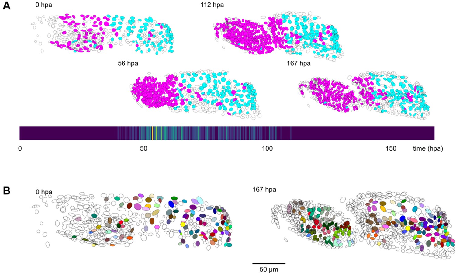
Cell lineages tracked during the time course of leg regeneration.

(A) Spatial and temporal distribution of dividing nuclei in the regenerating leg of *Parhyale* tracked over a 1-week time course (PH dataset), showing that cell proliferation is concentrated at the distal part of the regenerating leg stump and peaks after a period of proliferative quiescence, as described in Alwes et al., 2016. Top: Nuclei in lineages that contain at least one division are colored in magenta, nuclei in non-dividing lineages are in cyan, and nuclei in which the division status is undetermined are blank (see Materials and methods). Bottom: Heat map of the temporal distribution of nuclear divisions; hpa, hours post amputation. The number of divisions per 20-min time interval ranges from 0 (purple) to 9 (yellow). (B) Fate map of the regenerating leg of *Parhyale*, encompassing 109 fully tracked lineage trees (202 cells at 167 hpa). Each clone is assigned a unique color and contains 1–9 cells at 167 hpa. Partly tracked nuclei are blank. In both panels, the amputation plane (distal end of the limb) is located on the left.

Materials and methods

Image datasets

Request a detailed protocol

The PH dataset (dataset li13) was obtained by imaging a regenerating T4 leg of the crustacean Parhyale hawaiensis, based on the method described by Alwes et al., 2016; Figure 5—video 1. The imaging was carried out on a transgenic animal carrying the Mi(3xP3> DsRed; PhHS> H2B-mRFPRuby) construct (Wolff et al., 2018), in which nuclear-localised mRFPRuby fluorescent protein is expressed in all cells following heat-shock. The leg was amputated at the distal end of the carpus. Following the amputation, continuous live imaging over a period of 1 week was performed on a Zeiss LSM 800 confocal microscope equipped with a Plan-Apochromat 20 x/0.8 M27 objective (Zeiss 420650-9901-000), in a temperature control chamber set to 26 °C. Heat-shocks (45 minutes at 37 °C) were applied 24 hr prior to the amputation, and 65 and 138 hr post-amputation. Every 20 min we recorded a stack of 11 optical sections, with a z step of 2.48 microns. Voxel size (in xyz) was 0.31 × 0.31 x 2.48 microns.

The CE1 and CE2 datasets (Murray et al., 2008) and the MDA231 dataset were obtained via the Cell Tracking Challenge (Ulman et al., 2017) (datasets Fluo-N3DH-CE and Fluo-C3DL-MDA231). The ORG1 and ORG2 datasets were obtained from de Medeiros, 2021 and Kok et al., 2020, respectively. Additional datasets used to train the generic models (see Supplementary file 3) were obtained from the Cell Tracking Challenge (Ulman et al., 2017).

ELEPHANT platform architecture

Request a detailed protocol

ELEPHANT implements a client-server architecture (Figure 1—figure supplement 1), which can be set up on the same computer or on multiple connected computers. This architecture brings flexibility: allowing the client to run Mastodon (implemented in Java) while the deep learning module is implemented separately using Python, and releasing the client computer from the requirements of high GPU needed to implement deep learning. The client side is implemented by extending Mastodon, a framework for cell tracking built upon the SciJava ecosystem (https://scijava.org/) and is available as a Fiji (Schindelin et al., 2012) plugin. Combining the BigDataViewer (Pietzsch et al., 2015) with an efficient memory access strategy (https://github.com/mastodon-sc/mastodon/blob/master/doc/trackmate-graph.pdf), Mastodon enables fast and responsive user interaction even for very large datasets. ELEPHANT leverages the functionalities provided by Mastodon, including the functions for manual annotation of nuclei, and extends them by implementing modules for deep learning-based algorithms.

The server side is built using an integrated system of a deep learning library (PyTorch Paszke et al., 2019), tools for tensor computing and image processing (NumPy Harris et al., 2020), SciPy (Virtanen et al., 2020), Scikit Image (van der Walt et al., 2014), and web technologies (Nginx, uWSGI, Flask). The client and the server communicate by Hypertext Transfer Protocol (HTTP) and JavaScript Object Notation (JSON). To reduce the amount of data exchanged between the client and the server, the image data is duplicated and stored in an appropriate format on each side. An in-memory data structure (Redis) is used to organize the priorities of the HTTP requests sent by the client. A message queue (RabbitMQ) is used to notify the client that the model is updated during training. The client software is available as an extension on Fiji (https://github.com/elephant-track/elephant-client). The server environment is provided as a Docker container to ensure easy and reproducible deployment (https://github.com/elephant-track/elephant-server). The server can also be set up with Google Colab in case the user does not have access to a computer that satisfies the system requirements.

Computer setup and specifications

Request a detailed protocol

In this study, we set up the client and the server on the same desktop computer (Dell Alienware Aurora R6) with the following specifications: Intel Core i7-8700K CPU @3.70 GHz, Ubuntu 18.04, 4 × 16 GB DDR4 2,666 MHz RAM, NVIDIA GeForce GTX 1080 Ti 11 GB GDDR5X (used for deep learning), NVIDIA GeForce GTX 1650 4 GB GDDR5, 256 GB SSD and 2 TB HDD. System requirements for the client and the server are summarized in the user manual (https://elephant-track.github.io/).

Dataset preparation

Request a detailed protocol

Images were loaded in the BigDataViewer (BDV, Pietzsch et al., 2015) format on the client software. The CE1, CE2, ORG1, ORG2, and MDA231 datasets were converted to the BDV format using the BigDataViewer Fiji plugin (https://imagej.net/BigDataViewer) without any preprocessing. Because the PH dataset showed non-negligible variations in intensity during long-term imaging, the original 16-bit images were intensity normalized per timepoint before conversion to the BDV format, for better visualization on Mastodon. In this normalization, the intensity values were re-scaled so that the minimum and maximum values at each timepoint become 0 and 65535, respectively. The PH dataset also showed 3D drifts due to heat-shocks. The xy drifts were corrected using an extended version of image alignment tool (Tseng et al., 2011) working as an ImageJ (Schneider et al., 2012) plugin, where the maximum intensity projection images were used to estimate the xy displacements, subsequently applied to the whole image stack (https://github.com/elephant-track/align-slices3d). The z drifts were corrected manually by visual inspection using Fiji.

On the server, images, annotation labels and outputs were stored in the Zarr format, allowing fast read/write access to subsets of image data using chunk arrays (Moore et al., 2021). At the beginning of the analysis, these data were prepared using a custom Python script that converts the original image data from HDF5 to Zarr and creates empty Zarr files for storing annotation labels and outputs (https://github.com/elephant-track/elephant-server). This conversion can also be performed from the client application. Generally, HDF5 is slower in writing data than Zarr, especially in parallelization, while they show comparable reading speeds (Moore et al., 2021).

Algorithm for detection

Request a detailed protocol

Detection of nuclei relies on three components: (i) a U-Net CNN that outputs probability maps for nucleus center, nucleus periphery, and background, (ii) a post-processing workflow that extracts nucleus center voxels from the probability maps, (iii) a module that reconstructs nuclei instances as ellipsoids. We designed a variation of 3D U-Net (Cicek et al., 2016) as illustrated in Figure 2—figure supplement 1. In both encoder and decoder paths, repeated sets of 3D convolution, ReLU activation (Nair and Hinton, 2010) and Group Normalization (Wu and He, 2020) are employed. Max pooling in 3D is used for successive downsampling in the encoder path, in each step reducing the size to half the input size (in case of anisotropy, maintaining the z dimension until the image becomes nearly isotropic). Conversely, in the decoder path, upsampling with nearest-neighbor interpolation is applied to make the dimensions the same as in the corresponding intermediate layers in the encoder path. As a result, we built a CNN with 5,887,011 trainable parameters. The weights are initialized with the Kaiming fan-in algorithm (He et al., 2015a) and the biases are initialized to zero for each convolution layer. For each group normalization layer, the number of groups is set as the smallest value between 32 and the number of output channels, and the weights and biases are respectively initialized to one and zero. When starting to train from scratch, the CNN is trained using the cropped out 3D volumes from the original image prior to training with annotations. In this prior training phase, a loss function $L_{p r i o r}$ is used that penalizes the addition of the following two mean absolute differences (MADs): (i) nucleus center probabilities c_i and the [0, 1] normalized intensity of the original image y_i, (ii) background probabilities b_i and the [0, 1] normalized intensity of the intensity-inverted image $1 - y_{i}$ where i stands for the voxel index of an input volume with $n$ voxels $i \in V := {1, 2, \dots, n}$ .

L_{p r i o r} = \frac{1}{n} \sum_{i = 1}^{n} | y_{i} - c_{i} | + \frac{1}{n} \sum_{i = 1}^{n} | (1 - y_{i}) - b_{i} |

The prior training is performed on three cropped out 3D volumes generated from the 4D datasets, where the timepoints are randomly picked, and the volumes are randomly cropped with random scaling in the range (0.8, 1.2). The training is iterated for three epochs with decreasing learning rates (0.01, 0.001, and 0.0001, in this order) with the Adam optimizer (Kingma and Ba, 2014). The prior training can be completed in ~20 s for each dataset.

Training with sparse annotations is performed in the following steps. First, the client application extracts the timepoint, 3D coordinates and covariances representing ellipsoids of all the annotated nuclei in the specified time range. Subsequently, these data, combined with user-specified parameters for training, are embedded in JSON and sent to the server in an HTTP request. On the server side, training labels are generated from the received information by rendering nucleus center, nucleus periphery, background and unlabelled voxels with distinct values. The background labels are generated either by explicit manual annotation or intensity thresholding, where the threshold value is specified by the user, resulting in the label images as shown in Figure 2A. To render ellipsoids in the anisotropic dimension, we extended the draw module in the scikit-image library (van der Walt et al., 2014) (https://github.com/elephant-track/elephant-server). Training of the CNN is performed using the image volumes as input and the generated labels as target with a loss function $L_{v c l a s s}$ that consists of three terms: (i) a class-weighted negative log-likelihood (NLL) loss, (ii) a term computed as one minus the dice coefficient for the nucleus center voxels, and (iii) a term that penalizes the roughness of the nucleus center areas. We used the empirically-defined class weights $w c$ for the NLL loss: $n u c l e u s c e n t e r = 10$ , $n u c l e u s p e r i p h e r y = 10$ , $b a c k g r o u n d = 1$ ; the unlabelled voxels are ignored. The first two terms accept different weights for the true annotations $w t$ (i.e. true positive and true negative) and the false annotations $w f$ (i.e. false positive and false negative). The third term is defined as the MAD between the voxel-wise probabilities for nucleus center and its smoothed representations, which are calculated by the Gaussian filter with downsampling ( $D o w n$ ) and upsampling ( $U p$ ). Let i stand for the voxel index of an input volume with $n$ voxels $i \in V := {1, 2, \dots, n}$ , x_i for the input voxel value, $h_{i}$ for the output from the CNN before the last activation layer for the three classes, $y_{i} \in Y := {1, 2, 3}$ for the voxel class label (1: nucleus center, 2: nucleus periphery, 3: background, respectively), and $z_{i} \in Z := {t r u e, f a l s e, u n l a b e l e d}$ for the voxel annotation label. We define the following subsets: the voxel index with true labels $T = {i ∣ i \in V, z_{i} = t r u e}$ , with false labels $F = {i ∣ i \in V, z_{i} = f a l s e}$ , and the nucleus center $C = {i ∣ i \in V, y_{i} = 1}$ . In the calculation of the $L_{d i c e}$ , a constant $ϵ = 0.000001$ is used to prevent zero division. Using these components and the empirically-defined weights for each loss term ( $α = 1, β = 5, γ = 1$ ), we defined the $L_{v c l a s s}$ as below.

L_{v c l a s s} = α L_{n l l} + β L_{d i c e} + γ L_{s m o o t h}

L_{n l l} = w t \frac{\sum_{i \in T} (N L L (h_{i}, y_{i}) \cdot w c [y_{i}])}{\sum_{i \in T} w c [y_{i}]} + w f \frac{\sum_{i \in F} (N L L (h_{i}, y_{i}) \cdot w c [y_{i}])}{\sum_{i \in F} w c [y_{i}]}

\begin{array}{ll} L_{d i c e} = w t (1 - \frac{2 \sum_{i \in T} (P r o b (h_{i}, 1) \cdot O n e h o t (y_{i}, 1))}{m a x (\sum_{i \in T} ({(P r o b (h_{i}, 1))}^{2} + {(O n e h o t (y_{i}, 1))}^{2}), ϵ)}) \\ + w f (1 - \frac{2 \sum_{i \in F} (P r o b (h_{i}, 1) \cdot O n e h o t (y_{i}, 1))}{m a x (\sum_{i \in F} ({(P r o b (h_{i}, 1))}^{2} + {(O n e h o t (y_{i}, 1))}^{2}), ϵ)}) \end{array}

L_{s m o o t h} = \frac{1}{n} \sum_{i \in V} | P r o b (h_{i}, 1) - U p (D o w n (P r o b (h_{i}, 1))) |

P r o b (h, c) = \frac{e x p (h [c])}{\sum_{j = 1}^{3} e x p (h [j])}

N L L (h, y) = - \log (P r o b (h, y))

O n e h o t (y_{i}, c) = {\begin{cases} 0 & (y_{i} \neq c) \\ 1 & (y_{i} = c) \end{cases}

In the analyses shown in Figure 3 and its supplements 1 and 2, the following loss functions are updated to make them more robust using normalization, which are employed in the current version of software.

L_{v c l a s s} = \frac{α L_{n l l} + β L_{d i c e} + γ L_{s m o o t h}}{α + β + γ}

L_{n l l} = \frac{n (T) w t}{n (T) w t + n (F) w f} \frac{\sum_{i \in T} (N L L (h_{i}, y_{i}) \cdot w c [y_{i}])}{\sum_{i \in T} w c [y_{i}]} + \frac{n (F) w f}{n (T) w t + n (F) w f} \frac{\sum_{i \in F} (N L L (h_{i}, y_{i}) \cdot w c [y_{i}])}{\sum_{i \in F} w c [y_{i}]}

\begin{array}{ll} L_{d i c e} = \frac{n (T) w t}{n (T) w t + n (F) w f} (1 - \frac{2 \sum_{i \in T} (P r o b (h_{i}, 1) \cdot O n e h o t (y_{i}, 1))}{m a x (\sum_{i \in T} ({(P r o b (h_{i}, 1))}^{2} + {(O n e h o t (y_{i}, 1))}^{2}), ϵ)}) \\ + \frac{n (F) w f}{n (T) w t + n (F) w f} (1 - \frac{2 \sum_{i \in F} (P r o b (h_{i}, 1) \cdot O n e h o t (y_{i}, 1))}{m a x (\sum_{i \in F} ({(P r o b (h_{i}, 1))}^{2} + {(O n e h o t (y_{i}, 1))}^{2}), ϵ)}) \end{array}

Training of the CNN is performed on the image volumes generated from the 4D datasets, where the volumes are randomly cropped with/without random scaling, random contrast, random flip and random rotation, which are specified at runtime. There are two modes for training: (i) an interactive mode that trains a model incrementally, as the annotations are updated, and (ii) a batch mode that trains a model with a fixed set of annotations. In the interactive training mode, sparse annotations in a given timepoint are used to generate crops of image and label volumes, with which training is performed using the Adam optimizer with a learning rate specified by the user. In the batch training mode, a set of crops of image and label volumes per timepoint is generated each iteration, with which training is performed for a number of epochs specified by the user (ranging from 1 to 1000) using the Adam optimizer with the specified learning rates. In the prediction phase, the input volume can be cropped into several blocks with smaller size than the original size to make the volume can be cropped into several blocks with smaller size than the original size to make the input data compatible with available GPU memory. To stitch the output blocks together, the overlapping regions are seamlessly blended by weighted linear blending.

In post-processing for the CNN output, voxel-wise probabilities for nucleus center class are denoised by subtracting edges of background class that are calculated with the Gaussian filter and the Prewitt operation for each z-slice. After denoising, the voxels with nucleus center probabilities greater than a user defined value are thresholded and extracted as connected components, which are then represented as ellipsoids (from their central moments). These ellipsoids representing the nucleus center regions are enlarged so that they cover the original nucleus size (without excluding its periphery). The ellipsoids with radii smaller than $r_{m i n}$ are removed and the radii are clamped to $r_{m a x}$ specified by the user, generating a list of center positions and covariances that can be used to reconstruct the nuclei. On the client application, the detection results are converted to Mastodon spots and rendered on the BDV view, where the existing and predicted nuclei are tagged based on their status: labelled as ‘true positive’ (positive and predicted), ‘false negative’ (positive and not predicted), ‘true negative’ (negative and not predicted), ‘false positive’ (negative and predicted), and ‘non-validated’ (newly predicted). These labels can be visualized when running ELEPHANT in the advanced color mode (in basic color mode true positives and false negatives are visualized as ‘accepted’ and false positives and true negatives as ‘rejected’). If more than one nucleus is predicted within a user-specified threshold $d_{s u p}$ , the one with human annotation is given priority, followed by the one with the largest volume.

Algorithm for linking

Request a detailed protocol

Linking of nuclei relies on two components: (i) estimation of the positions of nuclei at the previous timepoint by optical flow estimation using deep learning, which is skipped in the case of the nearest neighbor algorithm without flow support, (ii) association of nuclei based on the nearest neighbor algorithm. We designed a variation of 3D U-Net for flow estimation as illustrated in Figure 4—figure supplement 1. In the encoder path, the residual blocks (He et al., 2015b) with 3D convolution and LeakyReLU (Maas et al., 2013) activation are applied, in which the outputs are divided by two after the sum operation to keep the consistency of the scale of values. In the decoder path, repeated sets of 3D convolution and LeakyReLU activation are employed. Downsampling and upsampling are applied as described for the detection model. Tanh activation is used as a final activation layer. As a result, we built a CNN with 5,928,051 trainable parameters. The weights and biases for convolution layers are initialized as described for the detection model. Training of the flow model with sparse annotations is performed in a similar way as for the detection model. First, on the client application, for each annotated link, which connects the source and target nuclei, the following information gets extracted: the timepoint, the backward displacements in each of the three dimensions, and the properties of the target nucleus (3D coordinates and covariances). Subsequently, these data, combined with parameters for training, are embedded in JSON and sent to the server in an HTTP request. On the server side, flow labels are generated from the received information by rendering backward displacements for each target nucleus in each of three dimensions, where the displacements are scaled to fit the range (–1, 1). In this study, we used fixed scaling factors (1/80, 1/80, 1/10) for each dimension, but they can be customized to the target dataset. Foreground masks are generated at the same time to ignore unlabelled voxels during loss calculation. Ellipsoid rendering is performed as described for the detection training. Training of the CNN for flow estimation is performed using the two consecutive image volumes $(I_{t - 1}, I_{t})$ as input, and the generated label as target. A loss function $L_{f l o w}$ is defined with the following three terms; (i) a dimension-weighted MAD between the CNN outputs and the flow labels, (ii) a term computed as one minus the structural similarity (SSIM) (Wang et al., 2004) of $I_{t - 1}$ and ${\tilde{I}}_{t}$ , where the estimated flow is applied to $I_{t}$ (Ilg et al., 2017), (iii) a term penalizing the roughness of the CNN outputs. Let i stand for the voxel index of an input volume with $n$ voxels $i \in V := {1, 2, \dots, n}$ , x_i for the input voxel value, $\hat{y}$ for the output of the CNN, $y$ for the flow label, $m \in M \subset V$ for the index of the annotated voxels, $d \in D := {0, 1, 2}$ for the dimension index for three dimensions and $w d$ for the dimension weights. In the SSIM calculation, we defined a function $G a u s s$ as a 3D Gaussian filter with the window size 7 × 7 x 3 and standard deviation of 1.5. Using these components and the empirically defined weights for each loss term $(α = 1, β = 0.0001, γ = 0.0001)$ , we defined the $L_{f l o w}$ as below.

L_{f l o w} = α L_{m a d} + β L_{s s i m} + γ L_{s m o o t h}

L_{m a d} = \frac{1}{n} \sum_{d \in D} w d_{d} \sum_{m \in M} | y_{m d} - {\hat{y}}_{m d} |

L_{s s i m} = 1 - S S I M (I_{t - 1}, {\hat{I}}_{t})

L_{s m o o t h} = \frac{1}{3 n} \sum_{i \in V} \sum_{d \in D} | {\hat{y}}_{i d} - U p (D o w n ({\hat{y}}_{i d})) |

μ_{I_{1}} = G a u s s (I_{1}), μ_{I_{2}} = G a u s s (I_{2})

σ_{I_{1}}^{2} = G a u s s (I_{1}^{2}) - μ_{I_{1}}^{2}, σ_{I_{2}}^{2} = G a u s s (I_{2}^{2}) - μ_{I_{2}}^{2}, σ_{I_{1} I_{2}} = G a u s s (I_{1} I_{2}) - μ_{I_{1}} μ_{I_{2}}

S S I M (I_{1}, I_{2}) = \frac{(2 μ_{I_{1}} μ_{I_{2}} + C_{1}) (2 σ_{I_{1} I_{2}} + C_{2})}{(μ_{I_{1}}^{2} + μ_{I_{2}}^{2} + C_{1}) (σ_{I_{1}}^{2} + σ_{I_{2}}^{2} + C_{2})}

, where $C_{1} = 0.0001$ and $C_{2} = 0.0009$ . In the current version of software, the following loss functions are updated to make them more robust using normalization.

L_{f l o w} = \frac{α L_{m a d} + β L_{s s i m} + γ L_{s m o o t h}}{α + β + γ} (α = 1, β = 0.01, γ = 0.01)

L_{m o d} = \frac{1}{n (M)} \sum_{d \in D} \frac{w d_{d}}{\sum_{d \in D} w d_{d}} \sum_{m \in M} | y_{m d} - {\hat{y}}_{m d} |

The training is performed on the image volumes generated from the 4D datasets, where the sets of two consecutive images and corresponding flow labels are randomly cropped with/without random scaling and random rotation, which are specified at runtime. The training is performed for a fixed number of epochs using the Adam optimizer and with learning rates specified by the user, generating a set of images and labels for each timepoint in each epoch. The CNN outputs are rescaled to the original physical scale and used to calculate the estimated coordinate of each nucleus center at the previous timepoint. Let $K \subset V$ stands for a subset of voxel index of a nucleus and $p$ for its center coordinate. Using the output of the CNN $\hat{y}$ and the scaling factor $s$ , the estimated coordinate at the previous timepoint $\hat{p}$ is calculated.

\hat{p} = p + \frac{s}{n (K)} \sum_{k \in K} {\hat{y}}_{k}

These estimated coordinates are subsequently used to find the parent of the nucleus at the previous timepoint by the nearest neighbor algorithm (a similar concept was introduced for 2D phase contrast microscopy data; Hayashida and Bise, 2019; Hayashida et al., 2020). The pairs with a distance smaller than $d_{s e a r c h}$ are considered as link candidates, where the closer the Euclidean distance between the two points, the higher their priority of being the correct link. Each nucleus accepts either one or two links, determined by the estimated displacements and actual distances. Briefly, given that a single nucleus has two possible links, it can accept both if at least one of the estimated displacements is larger than the threshold $d_{d i s p}$ or both distances are smaller than the threshold $d_{d i s t}$ . In this study, we used ad hoc thresholds $d_{d i s p} = 1.0$ and $d_{d i s t} = 1.0$ . If there are competing links beyond the allowed maximum of two links, the links with smaller $d_{d i s p}$ are adopted and the remaining nucleus looks for the next closest nucleus up to $N_{m a x}$ neighbors. The links are generated by repeating the above procedure until all the nuclei get linked or the iteration count reaches to five. We optionally implement an interpolation algorithm, in which each orphan nucleus tries to find its source up to $T_{m a x}$ timepoints back and is linked with a nucleus at the estimated coordinate based on the flow prediction, interpolating the points in between.

Preparation of generic pre-trained models and fine-tuning with sparse annotations (Figure 3)

Request a detailed protocol

The generic pre-trained models for each dataset were trained on the datasets summarized in Supplementary file 3. Training of the detection models was performed with volumes of 384 × 384 x 16 voxels or smaller, which were generated by preprocessing with random flip in each dimension, random scaling in the range (0.5, 2), random cropping and random contrast in the range (0.5, 1). In the label generation step, the center ratio was set to 0.4 and the background threshold was set to 1 (i.e. all voxels without manual annotations are background) for the Cell Tracking Challenge datasets (Fluo-C3DH-A549, Fluo-C3DH-H157, Fluo-C3DL-MDA231, Fluo-N3DH-CE and Fluo-N3DH-CHO), and to 0.03 for the PH dataset. The labels for the Cell Tracking Challenge datasets were automatically generated from the silver-standard corpus (silver truth). We trained the models for up to 200 epochs starting from scratch using the Adam optimizer with the learning rate of 5 × 10^–3, where each epoch contained randomly selected 10 pre-processed volumes from each dataset. Validation was performed after each epoch using randomly selected five timepoints from each dataset. In the validation phase, image volumes were fed into the model using blocks with size 512 × 512 x 24 or smaller, and the outputs were stitched together to reconstruct the whole volume. For each condition, the model with the highest score in the validation data was finally adopted. At the start of each epoch, the model parameters were set to the ones that had previously produced the highest scores on the validation data. The parameters for training and validation are summarized in Supplementary file 5. Fine-tuning of the model was performed as follows: (i) 3–10 sparse annotations were added at the points where the pre-trained model failed in detection (Figure 3 middle), (ii) we trained the models for 10 epochs starting from the pre-trained model parameters with volumes of 384 × 384 x 16 voxels or smaller. These volumes were generated by preprocessing with random flip in each dimension, random scaling in the range (0.5, 2), random cropping and random contrast in the range (0.5, 1), using the Adam optimizer with the learning rate of 0.01 or 0.001, where each epoch contained five randomly cropped volumes. The pre-trained model and the fine-tuned model were applied to each dataset with parameters summarized in Supplementary file 6. The evaluation scores were calculated based on the detection criterion of ELEPHANT, which recognizes that a prediction is correct if the distance between the prediction and the manual annotation is less than $d_{s u p}$ .

Comparison between ELEPHANT and StarDist3D (Figure 3 – Supplement 1)

Request a detailed protocol

The ELEPHANT detection model is the same as the one used in Figure 3—figure supplement 2. For training of the StarDist3D (Weigert et al., 2020) segmentation model, a single volume of the CE1 dataset (timepoint = 100) with the fully labelled instance segmentation annotations (93 nuclei) was used for training, and another volume of the CE1 dataset (timepoint = 101) with the fully labelled instance segmentation annotations (95 nuclei) was used for validation during training. The instance segmentation annotations were taken from the silver-standard corpus (silver truth) in the Cell Tracking Challenge. Training of the StarDist3D model was performed with the parameters summarized in Supplementary file 4. The model with the best performance in the validation data was selected for comparison. The trained ELEPHANT and StarDist3D models were applied to a single volume (timepoint = 100) of the CE2 dataset to generate the output for comparison (Figure 3—figure supplement 1). The DET scores were calculated by the evaluation software provided by the Cell Tracking Challenge using the gold-standard corpus (gold truth).

Evaluation of overfitting of the detection model (Figure 3 – Supplement 2)

Request a detailed protocol

A single volume of the CE1 dataset (timepoint = 100) with sparse annotations (10 nuclei) was used for training, and a single volume of the fully labelled CE2 dataset (timepoint = 100) was used for validation. Training of the detection model was performed using 384 × 384 x 16 cropped-out image volumes generated by preprocessing with random flip in each dimension, random scaling in the range (0.5, 2), random cropping and random contrast in the range (0.5, 1). In the label generation step, the center ratio was set to 0.4 and the background threshold was set to 0 (i.e. all voxels without manual annotations are ignored). We trained a model for 500 epochs starting from scratch using the Adam optimizer with the learning rate of 5 × 10^–4, where each epoch contained five pre-processed volumes. Training and validation losses were recorded at the end of each epoch (Figure 3—figure supplement 2, bottom left). The detection model trained for 500 epochs was tested on the CE1 dataset (partially-seen data; Figure 3—figure supplement 2, top right) and the CE2 dataset (unseen data; Figure 3—figure supplement 2, bottom right). In the prediction phase, the input volumes were cropped into 2 × 2 x 2 blocks with size 544 × 384 x 28 for CE1 or 544 × 384 x 24 for CE2, and stitched together to reconstruct the whole image of 708 × 512 x 35 for CE1 or 712 × 512 x 31 for CE2. In the postprocessing of the prediction for detection, a threshold for the nucleus center probabilities were set to 0.5, and $r_{m i n}$ , $r_{m a x}$ and $d_{s u p}$ were set to 0.5 µm, 3 µm, and 2 µm respectively. The evaluation scores were calculated in the same way as described in the previous section.

Detection and tracking in the CE datasets (Figures 2 and 4)

Request a detailed protocol

On the CE1 and CE2 datasets, training of detection and flow models was performed with volumes of 384 × 384 x 16 voxels that were generated by preprocessing with random scaling in the range (0.5, 2) and random cropping. For training of a detection model, preprocessing with random contrast in the range (0.5, 1) was also applied. In the label generation step, the center ratio was set to 0.3 and the background threshold was set to 0.1 and 1 (i.e. all voxels without manual annotations are background). In the interactive training of detection models, 10 labelled cropped out volumes were generated per iteration, with which training was performed using the Adam optimizer with a learning rate between 5 × 10^–5 and 5 × 10^–6. In the batch training of detection models, training was performed for 100 epochs using the Adam optimizer with learning rates of 5 × 10^–5. In the training of a flow model, training was performed for 100 epochs using the Adam optimizer with learning rates of 5 × 10^–5 for the first 50 epochs and 5 × 10^–6 for the last 50 epochs. $w t$ and $w f$ were set to 1 and 5, respectively, and $w d$ was set to (1/3, 1/3, 1/3). In the prediction phase, the input volumes were cropped into 2 × 2 x 2 blocks with size 544 × 384 x 28 for CE1 or 544 × 384 x 24 for CE2, and stitched together to reconstruct the whole image of 708 × 512 x 35 for CE1 or 712 × 512 x 31 for CE2. In the preprocessing of the prediction for detection, we corrected the uneven background levels across the z-slices by shifting the slice-wise median value to the volume-wise median value. In the postprocessing of the prediction for detection, a threshold for the nucleus center probabilities were set to 0.3, and $r_{m i n}$ and $r_{m a x}$ , $d_{s u p}$ were set to 1 µm, 3 µm and 1 µm, respectively. In the nearest-neighbor linking with/without flow prediction, $d_{s e a r c h}$ was set to 5 µm and $N_{m a x}$ was set to 3. In the results submitted to the Cell Tracking Challenge (Table 1), the suppression of detections with $d_{s u p}$ was not applied, and the linking was performed by the nearest-neighbor linking with flow support and an optional interpolation module, where $T_{m a x}$ was set to 5.

Detection and tracking in the PH dataset

Request a detailed protocol

On the PH dataset, training of detection and flow models was performed with volumes of 384 × 384 x 12 voxels generated by preprocessing with random rotation in the range of ±180 degrees and random cropping. For training a detection model, preprocessing with random contrast in the range (0.5, 1) was also applied. In the label generation step, the center ratio was set to 0.3, and the background threshold was set to 0.03. In the interactive training of a detection model, 10 crops of image and label volumes were generated per iteration, with which training was performed using the Adam optimizer with a learning rate between 5 × 10^–5 and 5 × 10^–6. In the batch training of a detection model, training was performed for 100 epochs using the Adam optimizer with learning rates of 5 × 10^–5. In the training of a flow model, training was performed for 100 epochs using the Adam optimizer with learning rates of 5 × 10^–5 for the first 50 epochs and 5 × 10^–6 for the last 50 epochs. $w t$ and $w f$ were set to 1 and 3, respectively, and $w d$ was set to (1, 1, 8). In the prediction phase, the input volumes were fed into the CNNs without cropping or further preprocessing. In the postprocessing of the prediction for detection, a threshold for the $n u c l e u s c e n t e r$ probabilities were set to 0.3, and $r_{m i n}$ , $r_{m a x}$ and $d_{s u p}$ were set to 1 µm, 3 µm and 5 µm respectively. In the nearest-neighbor linking with/without flow prediction, $d_{s e a r c h}$ was set to 5 µm and $N_{m a x}$ was set to 3.

Analysis of CE and PH datasets

Request a detailed protocol

On the CE1 and CE2 datasets, the detection and link annotations were made starting from timepoint 0 and proceeding forward until timepoints 194 (CE1) and 189 (CE2), respectively. In the CE1 dataset, the detection was made from scratch, based on manual annotation and incremental training, and the linking was performed by the nearest neighbor algorithm without flow prediction. After completing annotation from timepoint 0 to 194 on the CE1 dataset, the detection and flow models were trained by the batch mode with the fully labelled annotations. In the CE2 dataset, the detection was performed in a similar way as for CE1, by extending the model trained with CE1, and the linking was performed by the nearest neighbor algorithm with flow support using the pre-trained model followed by proofreading. Incremental training of the detection model was performed when there were annotations from nuclei that were not properly predicted.

On the PH dataset, the annotations were made by iterating the semi-automated workflow. In general, the nuclei with high signal-to-noise ratio (SNR) were annotated early, while the nuclei with low SNR were annotated in a later phase. The detection model was updated frequently to fit the characteristics of each region and timepoint being annotated, while the flow model was updated less frequently. The CE1 dataset was used to evaluate the speed of detection and validation (Figure 2B). All workflows started at timepoint 0 and proceeded forward in time, adding and/or validating all the nuclei found in each timepoint. To evaluate the manual workflow, we annotated nuclei using hotkeys that facilitate the annotation of a given nucleus at successive timepoints. To evaluate the ELEPHANT from scratch workflow, we performed prediction with the latest model, followed by proofreading, including add, modify, or delete operations, and incremental training. At each timepoint, the model was updated with the new annotations added manually or by proofreading. To evaluate the ELEPHANT pre-trained workflow, we performed predictions with a model trained on the CE2 dataset, followed by proofreading without additional training. The numbers of validated nuclei associated with time were counted from the log data. We measured the counts over 30 min after the start of each workflow and plotted them in Figure 2B.

To compare the linking performances (Figure 4C), we trained the flow model with 1,162 validated links, including 18 links corresponding to 9 cell divisions, from 108 lineage trees collected between timepoints 150 and 159. It took around 30 hr to train the flow model from scratch using these links. Starting from a pre-trained model, the training time can be decreased to a few minutes, providing a major increase in speed compared with training from scratch (Supplementary file 2).

The results shown in A and BFigure 5A, B were generated based on the tracking results with 260,600 validated nuclei and 259,071 validated links. In the analysis for Figure 5A, nuclei were categorised as dividing or non-dividing depending on whether the lineages to which they belong contain at least one cell division or not during the period of cell proliferation (timepoints 100–350). Nuclei that did not meet these criteria were left undetermined. For Figure 5B, the complete lineages of 109 nuclei were tracked through the entire duration of the recording, from 0 to 167 hr post-amputation, with no missing links.

Evaluation of cell tracking performance

Request a detailed protocol

We submitted our results and executable software to the Cell Tracking Challenge organizers, who evaluated our algorithm’s performance, validated its reproducibility using the executable software that we submitted, and provided us with the scores. The details of the detection accuracy (DET), tracking accuracy (TRA), and segmentation accuracy (SEG) metrics can be found in the original paper (Matula et al., 2015) and the website (http://celltrackingchallenge.net/evaluation-methodology/). Briefly, the DET score evaluates how many split, delete, and add operations are required to achieve the ground truth starting from the predicted nuclei, reflecting the accuracy of detection; the TRA score evaluates how many split, delete, and add operations for nuclei, and delete, add, and alter the semantics operations for links are required to reconstruct the ground truth lineage trees from the predicted lineage trees, reflecting the accuracy of linking; the SEG score evaluates the overlap of the detected ellipsoids with fully segmented nuclei, reflecting the precision of nucleus segmentation. All three scores range from 0 (poorest) to 1 (best).

Data availability

Request a detailed protocol

The CE1, CE2, and MDA231 datasets are available from the Cell Tracking Challenge website: http://celltrackingchallenge.net/3d-datasets/. The ORG1 and ORG2 datasets were obtained from de Medeiros, 2021 and Kok et al., 2020, respectively. The following files are available at https://doi.org/10.5281/zenodo.4630933: (i) the tracking results shown in Figure 4B, (ii) the PH dataset and its tracking results, and (iii) deep-learning model parameters for the CE and PH datasets.

Code availability

Request a detailed protocol

The source code for the ELEPHANT client is available at https://github.com/elephant-track/elephant-client (Sugawara, 2021c copy archived at swh:1:rev:449f9ff8ad17ce75f355e18f815653ec0aa4bbb8), for the ELEPHANT server at https://github.com/elephant-track/elephant-server (Sugawara, 2021a copy archived at swh:1:rev:8935febdbcb2e2d6ba2220ca139e765db44e6458), and for the Align Slices 3D + t extension ImageJ plugin at https://github.com/elephant-track/align-slices3d (Sugawara, 2021b copy archived at swh:1:rev:36c6cb6ccb7e308f9349ec26294d408c35be1ed7). The user manual for ELEPHANT is available at https://elephant-trackgithub.io/.

Data availability

The imaging datasets are available at https://doi.org/10.5281/zenodo.4630933. The source code for the ELEPHANT software is available at https://github.com/elephant-track.

The following data sets were generated

1. Sugawara, Çevrim and Averof
(2021) Zenodo
PH_li13 Zenodo.
https://doi.org/10.5281/zenodo.4630933

The following previously published data sets were used

1. Waterston Lab
(2008) Cell Tracking Challenge
ID Fluo-N3DH-CE. C. elegans developing embryo.

http://data.celltrackingchallenge.net/training-datasets/Fluo-N3DH-CE.zip
1. Kamm R
(2017) Cell Tracking Challenge
ID Fluo-C3DL-MDA231. MDA231 human breast carcinoma cells.

http://data.celltrackingchallenge.net/training-datasets/Fluo-C3DL-MDA231.zip

References

(2016) Live imaging reveals the progenitors and cell dynamics of limb regeneration
eLife 5:e19766.
https://doi.org/10.7554/eLife.19766
- PubMed
- Google Scholar
(2013) Fast and robust optical flow for time-lapse microscopy using super-voxels
Bioinformatics 29:373–380.
https://doi.org/10.1093/bioinformatics/bts706
- PubMed
- Google Scholar
(2019) 3-D Quantification of Filopodia in Motile Cancer Cells
IEEE Transactions on Medical Imaging 38:862–872.
https://doi.org/10.1109/TMI.2018.2873842
- PubMed
- Google Scholar
(2016)
Medical Image Computing and Computer-Assisted Intervention - MICCAI 2016

3D U-Net: Learning Dense Volumetric Segmentation from Sparse Annotation, Medical Image Computing and Computer-Assisted Intervention - MICCAI 2016, Springer International Publishing, 10.1007/978-3-319-46723-8.
- Google Scholar
1. Crocker JC
2. Grier DG
(1996) Methods of Digital Video Microscopy for Colloidal Studies
Journal of Colloid and Interface Science 179:298–310.
https://doi.org/10.1006/jcis.1996.0217
- Google Scholar
Conference
1. de Medeiros G
(2021) European Light Microscopy Initiative 2021
Multiscale light-sheet organoid imaging framework.
https://doi.org/10.22443/rms.elmi2021.90
- Google Scholar
(2010) Advanced level-set-based cell tracking in time-lapse fluorescence microscopy
IEEE Transactions on Medical Imaging 29:852–867.
https://doi.org/10.1109/TMI.2009.2038693
- PubMed
- Google Scholar
1. Harris CR
2. Millman KJ
3. van der Walt SJ
4. Gommers R
5. Virtanen P
6. Cournapeau D
7. Wieser E
8. Taylor J
9. Berg S
10. Smith NJ
11. Kern R
12. Picus M
13. Hoyer S
14. van Kerkwijk MH
15. Brett M
16. Haldane A
17. Del Río JF
18. Wiebe M
19. Peterson P
20. Gérard-Marchant P
21. Sheppard K
22. Reddy T
23. Weckesser W
24. Abbasi H
25. Gohlke C
26. Oliphant TE
(2020) Array programming with NumPy
Nature 585:357–362.
https://doi.org/10.1038/s41586-020-2649-2
- PubMed
- Google Scholar
Book
1. Hayashida J
2. Bise R
(2019)
Cell Tracking with Deep Learning for Cell Detection and Motion Estimation in Low-Frame-Rate

In: Shen D, editors. Cal Image Computing and Computer Assisted Intervention – MICCAI 2019. Springer International Publishing. pp. 397–405.
- Google Scholar
Conference
(2020) 2020 IEEE/CVF Conference on Computer Vision and Pattern Recognition
MPM: Joint Representation of Motion and Position Map for Cell Tracking. pp. 3823–3832.
https://doi.org/10.1109/CVPR42600.2020.00388
- Google Scholar
Conference
1. He K
2. Zhang X
3. Ren S
4. Sun J
(2015a) IEEE International Conference on Computer Vision
Delving Deep into Rectifiers: Surpassing Human-Level Performance on ImageNet Classification. pp. 1026–1034.
https://doi.org/10.1109/ICCV.2015.123
- Google Scholar
Preprint
1. He K
2. Zhang X
3. Ren S
4. Sun J
(2015b) Deep Residual Learning for Image Recognition
arXiv.

https://arxiv.org/abs/1512.03385
- Google Scholar
1. Horn BKP
2. Schunck BG
(1981) Determining optical flow
Artificial Intelligence 17:185–203.
https://doi.org/10.1016/0004-3702(81)90024-2
- Google Scholar
Conference
1. Ilg E
2. Mayer N
3. Saikia T
4. Keuper M
5. Dosovitskiy A
6. Brox T
(2017) 2017 IEEE Conference on Computer Vision and Pattern Recognition
FlowNet 2.0: Evolution of Optical Flow Estimation with Deep Networks. pp. 1647–1655.
https://doi.org/10.1109/CVPR.2017.179
- Google Scholar
Preprint
1. Kingma DP
2. Ba J
(2014) Adam: A Method for Stochastic Optimization
arXiv.

https://arxiv.org/abs/1412.6980
- Google Scholar
1. Kok RNU
2. Hebert L
3. Huelsz-Prince G
4. Goos YJ
5. Zheng X
6. Bozek K
7. Stephens GJ
8. Tans SJ
9. van Zon JS
(2020) OrganoidTracker: Efficient cell tracking using machine learning and manual error correction
PLOS ONE 15:e0240802.
https://doi.org/10.1371/journal.pone.0240802
- PubMed
- Google Scholar
Conference
1. Lucas BD
2. Kanade T
(1981)
Proceedings of the 7th international joint conference on Artificial intelligence - Volume 2 IJC

An iterative image registration technique with an application to stereo vision. pp. 674–679.
- Google Scholar
Conference
1. Maas AL
2. Hannun AY
3. Ng AY
(2013)
CML Workshop on Deep Learning for Audio, Speech and Language Processing

Rectifier nonlinearities improve neural network acoustic models.
- Google Scholar
(2015) Global linking of cell tracks using the Viterbi algorithm
IEEE Transactions on Medical Imaging 34:911–929.
https://doi.org/10.1109/TMI.2014.2370951
- PubMed
- Google Scholar
(2013) Segmentation and shape tracking of whole fluorescent cells based on the Chan-Vese model
IEEE Transactions on Medical Imaging 32:995–1006.
https://doi.org/10.1109/TMI.2013.2243463
- PubMed
- Google Scholar
1. Maška M
2. Ulman V
3. Svoboda D
4. Matula P
5. Matula P
6. Ederra C
7. Urbiola A
8. España T
9. Venkatesan S
10. Balak DMW
11. Karas P
12. Bolcková T
13. Streitová M
14. Carthel C
15. Coraluppi S
16. Harder N
17. Rohr K
18. Magnusson KEG
19. Jaldén J
20. Blau HM
21. Dzyubachyk O
22. Křížek P
23. Hagen GM
24. Pastor-Escuredo D
25. Jimenez-Carretero D
26. Ledesma-Carbayo MJ
27. Muñoz-Barrutia A
28. Meijering E
29. Kozubek M
30. Ortiz-de-Solorzano C
(2014) A benchmark for comparison of cell tracking algorithms
Bioinformatics 30:1609–1617.
https://doi.org/10.1093/bioinformatics/btu080
- PubMed
- Google Scholar
Software
1. Mastodon Science
(2021) mastodon, version 2f1572c
GitHub.

https://github.com/mastodon-sc/mastodon
(2015) Cell Tracking Accuracy Measurement Based on Comparison of Acyclic Oriented Graphs
PLOS ONE 10:e0144959.
https://doi.org/10.1371/journal.pone.0144959
- PubMed
- Google Scholar
1. Moen E
2. Bannon D
3. Kudo T
4. Graf W
5. Covert M
6. Van Valen D
(2019) Deep learning for cellular image analysis
Nature Methods 16:1233–1246.
https://doi.org/10.1038/s41592-019-0403-1
- PubMed
- Google Scholar
1. Moore J
2. Allan C
3. Besson S
4. Burel JM
5. Diel E
6. Gault D
7. Kozlowski K
8. Lindner D
9. Linkert M
10. Manz T
11. Moore W
12. Pape C
13. Tischer C
(2021) OME-NGFF: a next-generation file format for expanding bioimaging data-access strategies
Nature Methods 18:1496–1498.
https://doi.org/10.1038/s41592-021-01326-w
- PubMed
- Google Scholar
1. Murray JI
2. Bao Z
3. Boyle TJ
4. Boeck ME
5. Mericle BL
6. Nicholas TJ
7. Zhao Z
8. Sandel MJ
9. Waterston RH
(2008) Automated analysis of embryonic gene expression with cellular resolution in C. elegans
Nature Methods 5:703–709.
https://doi.org/10.1038/nmeth.1228
- PubMed
- Google Scholar
Conference
1. Nair V
2. Hinton GE
(2010)
ICML 2010 - Proceedings, 27th International Conference on Machine Learning

Rectified linear units improve Restricted Boltzmann machines.
- Google Scholar
1. Ouyang W
2. Aristov A
3. Lelek M
4. Hao X
5. Zimmer C
(2018) Deep learning massively accelerates super-resolution localization microscopy
Nature Biotechnology 36:460–468.
https://doi.org/10.1038/nbt.4106
- PubMed
- Google Scholar
Preprint
1. Paszke A
2. Gross S
3. Massa F
4. Lerer A
5. Bradbury J
6. Chanan G
7. Killeen T
8. Lin Z
9. Gimelshein N
10. Antiga L
11. Desmaison A
12. Köpf A
13. Yang E
14. DeVito Z
15. Raison M
16. Tejani A
17. Chilamkurthy S
18. Steiner B
19. Fang L
20. Bai J
(2019) PyTorch: An Imperative Style, High-Performance Deep Learning Library
arXiv.

https://arxiv.org/abs/1912.01703
- Google Scholar
(2015) BigDataViewer: visualization and processing for large image data sets
Nature Methods 12:481–483.
https://doi.org/10.1038/nmeth.3392
- PubMed
- Google Scholar
Book
(2015) U-Net: Convolutional Networks for Biomedical Image Segmentation
In: Ronneberger O, editors. Lecture Notes in Computer Science (Including Subseries Lecture Notes in Artificial Intelligence and Lecture Notes in Bioinformatics. Springer. pp. 234–241.
https://doi.org/10.1007/978-3-319-24574-4_28
- Google Scholar
(2020) Cell segmentation and tracking using CNN-based distance predictions and a graph-based matching strategy
PLOS ONE 15:e0243219.
https://doi.org/10.1371/journal.pone.0243219
- PubMed
- Google Scholar
1. Schindelin J
2. Arganda-Carreras I
3. Frise E
4. Kaynig V
5. Longair M
6. Pietzsch T
7. Preibisch S
8. Rueden C
9. Saalfeld S
10. Schmid B
11. Tinevez JY
12. White DJ
13. Hartenstein V
14. Eliceiri K
15. Tomancak P
16. Cardona A
(2012) Fiji: an open-source platform for biological-image analysis
Nature Methods 9:676–682.
https://doi.org/10.1038/nmeth.2019
- PubMed
- Google Scholar
(2012) NIH Image to ImageJ: 25 years of image analysis
Nature Methods 9:671–675.
https://doi.org/10.1038/nmeth.2089
- PubMed
- Google Scholar
Software
1. Sugawara K
(2021a) elephant server, version swh:1:rev:8935febdbcb2e2d6ba2220ca139e765db44e6458
Software Heritage.

https://archive.softwareheritage.org/swh:1:dir:a3028f2a4adb71c0cc6249963f0777c6198d8602;origin=https://github.com/elephant-track/elephant-server;visit=swh:1:snp:2efc080405dc4ba11998f598bb4e9e785f39d314;anchor=swh:1:rev:8935febdbcb2e2d6ba2220ca139e765db44e6458
Software
1. Sugawara K
(2021b) Align Slices 3D+t extension, version swh:1:rev:36c6cb6ccb7e308f9349ec26294d408c35be1ed7
Software Heritage.

https://archive.softwareheritage.org/swh:1:dir:663a99923602d153e97af69164cd6762ed80f51d;origin=https://github.com/elephant-track/align-slices3d;visit=swh:1:snp:d18a8bf98eee86f6fe757f2087dcca11b051f897;anchor=swh:1:rev:36c6cb6ccb7e308f9349ec26294d408c35be1ed7
Software
1. Sugawara K
(2021c) ELEPHANT: Tracking cell lineages in 3D by incremental deep learning, version swh:1:rev:449f9ff8ad17ce75f355e18f815653ec0aa4bbb8
SoftwareHeritage.

https://archive.softwareheritage.org/swh:1:dir:e69da53d731182d6c6ffcb97588396e59a472e4f;origin=https://github.com/elephant-track/elephant-client;visit=swh:1:snp:f7f13f47ba9af8edaef97291b89bc4825a63a1b9;anchor=swh:1:rev:449f9ff8ad17ce75f355e18f815653ec0aa4bbb8
1. Tseng Q
2. Wang I
3. Duchemin-Pelletier E
4. Azioune A
5. Carpi N
6. Gao J
7. Filhol O
8. Piel M
9. Théry M
10. Balland M
(2011) A new micropatterning method of soft substrates reveals that different tumorigenic signals can promote or reduce cell contraction levels
Lab on a Chip 11:2231–2240.
https://doi.org/10.1039/c0lc00641f
- PubMed
- Google Scholar
1. Ulman V
2. Maška M
3. Magnusson KEG
4. Ronneberger O
5. Haubold C
6. Harder N
7. Matula P
8. Matula P
9. Svoboda D
10. Radojevic M
11. Smal I
12. Rohr K
13. Jaldén J
14. Blau HM
15. Dzyubachyk O
16. Lelieveldt B
17. Xiao P
18. Li Y
19. Cho S-Y
20. Dufour AC
21. Olivo-Marin J-C
22. Reyes-Aldasoro CC
23. Solis-Lemus JA
24. Bensch R
25. Brox T
26. Stegmaier J
27. Mikut R
28. Wolf S
29. Hamprecht FA
30. Esteves T
31. Quelhas P
32. Demirel Ö
33. Malmström L
34. Jug F
35. Tomancak P
36. Meijering E
37. Muñoz-Barrutia A
38. Kozubek M
39. Ortiz-de-Solorzano C
(2017) An objective comparison of cell-tracking algorithms
Nature Methods 14:1141–1152.
https://doi.org/10.1038/nmeth.4473
- PubMed
- Google Scholar
(2014) scikit-image: image processing in Python
PeerJ 2:e453.
https://doi.org/10.7717/peerj.453
- PubMed
- Google Scholar
1. Virtanen P
2. Gommers R
3. Oliphant TE
4. Haberland M
5. Reddy T
6. Cournapeau D
7. Burovski E
8. Peterson P
9. Weckesser W
10. Bright J
11. van der Walt SJ
12. Brett M
13. Wilson J
14. Millman KJ
15. Mayorov N
16. Nelson ARJ
17. Jones E
18. Kern R
19. Larson E
20. Carey CJ
21. Polat İ
22. Feng Y
23. Moore EW
24. VanderPlas J
25. Laxalde D
26. Perktold J
27. Cimrman R
28. Henriksen I
29. Quintero EA
30. Harris CR
31. Archibald AM
32. Ribeiro AH
33. Pedregosa F
34. van Mulbregt P
35. SciPy 1.0 Contributors
(2020) SciPy 1.0: fundamental algorithms for scientific computing in Python
Nature Methods 17:261–272.
https://doi.org/10.1038/s41592-019-0686-2
- PubMed
- Google Scholar
(2004) Image quality assessment: from error visibility to structural similarity
IEEE Transactions on Image Processing 13:600–612.
https://doi.org/10.1109/tip.2003.819861
- PubMed
- Google Scholar
1. Weigert M
2. Schmidt U
3. Boothe T
4. Müller A
5. Dibrov A
6. Jain A
7. Wilhelm B
8. Schmidt D
9. Broaddus C
10. Culley S
11. Rocha-Martins M
12. Segovia-Miranda F
13. Norden C
14. Henriques R
15. Zerial M
16. Solimena M
17. Rink J
18. Tomancak P
19. Royer L
20. Jug F
21. Myers EW
(2018) Content-aware image restoration: pushing the limits of fluorescence microscopy
Nature Methods 15:1090–1097.
https://doi.org/10.1038/s41592-018-0216-7
- PubMed
- Google Scholar
Conference
1. Weigert M
2. Schmidt U
3. Haase R
4. Sugawara K
5. Myers G
(2020) 2020 IEEE Winter Conference on Applications of Computer Vision
Star-convex Polyhedra for 3D Object Detection and Segmentation in Microscopy. pp. 3655–3662.
https://doi.org/10.1109/WACV45572.2020.9093435
- Google Scholar
1. Wen C
2. Miura T
3. Voleti V
4. Yamaguchi K
5. Tsutsumi M
6. Yamamoto K
7. Otomo K
8. Fujie Y
9. Teramoto T
10. Ishihara T
11. Aoki K
12. Nemoto T
13. Hillman EMC
14. Kimura KD
(2021) 3DeeCellTracker, a deep learning-based pipeline for segmenting and tracking cells in 3D time lapse images
eLife 10:e59187.
https://doi.org/10.7554/eLife.59187
- PubMed
- Google Scholar
1. Wolff C
2. Tinevez JY
3. Pietzsch T
4. Stamataki E
5. Harich B
6. Guignard L
7. Preibisch S
8. Shorte S
9. Keller PJ
10. Tomancak P
11. Pavlopoulos A
(2018) Multi-view light-sheet imaging and tracking with the MaMuT software reveals the cell lineage of a direct developing arthropod limb
eLife 7:e34410.
https://doi.org/10.7554/eLife.34410
- PubMed
- Google Scholar
1. Wu Y
2. He K
(2020) Group Normalization
International Journal of Computer Vision 128:742–755.
https://doi.org/10.1007/s11263-019-01198-w
- Google Scholar

Decision letter

Mackenzie W Mathis

Reviewing Editor; EPFL, Switzerland
Aleksandra M Walczak

Senior Editor; École Normale Supérieure, France
Asim Iqbal

Reviewer; EPFL, Switzerland
Christian Tischer

Reviewer; EMBL, Germany

Our editorial process produces two outputs: (i) public reviews designed to be posted alongside the preprint for the benefit of readers; (ii) feedback on the manuscript for the authors, including requests for revisions, shown below. We also include an acceptance summary that explains what the editors found interesting or important about the work.

Decision letter after peer review:

Thank you for submitting your article "Tracking cell lineages in 3D by incremental deep learning" for consideration by eLife. Your article has been reviewed by 3 peer reviewers, and the evaluation has been overseen by a Reviewing Editor and Aleksandra Walczak as the Senior Editor. The following individuals involved in review of your submission have agreed to reveal their identity: Asim Iqbal (Reviewer #1); Christian Tischer (Reviewer #3).

The reviewers have discussed their reviews with one another, and the Reviewing Editor has drafted this to help you prepare a revised submission.

Essential revisions:

1) Please address the usability of the code (i.e., please see all three reviewers comments and try to address them).

2) Please address reviewer comments regarding if a 3DUNet is sufficient, and truly state of the art; please provide results comparing to other architectures (such as StarDist, as reviewer 2 points out, or other architectures, see reviewer 1). Also, please consider adding limitations around network options to the discussion.

3) Multiple reviewers have questions around the ellipse tracker – could you show this is best / alternatives for cells with other shapes, and please consider a limitation regarding this (i.e., I assume a neuron with a long axon would not be well fit by an ellipse).

Reviewer #1 (Recommendations for the authors):

– Consider moving figure 1 in supplementary and make figure 2 as figure 1.

– Add a block diagram to show how to use ELEPHANT step by step through an example.

– It would be nice to show training, validation curves of 3D U-Nets in the supplementary figures to confirm if there is no over-fitting in the models.

– Demonstrate the usage and performance of the framework on diverse examples in the main figures (e.g. Figure 2).

– Expand the Result section in the study.

Reviewer #2 (Recommendations for the authors):

More details about running the code: The specific link to the documentation was broken on github. I tried to go through the instructions in the readme, discovered that Mastodon installation requires java sdk (these instructions should be included for linux, windows and mac). Once java was installed the user needs to convert tiffs, like those from celltrackingchallenge.net, into bigdataviewer format. This procedure should be documented at least for the format provided on celltrackingchallenge. For instance, I opened a folder of tiffs in imageJ, converted to a stack, then saved as an xml. If there is a way to do this for instance from the command line it would be great for it to be documented. Next I opened the xml from inside mastodon (the window that pops up from "java -jar elephant-0.1.0-client.jar"). I was able to open bdv but when I tried to do anything in the elephant plugin it said connection refused. I was running the code on Ubuntu 18.04.

It would be helpful to include more discussion about the amount of data needed, and the amount of manual input. This tool has increased practical value if ~1 month of interactive tracking (as described in the paper) is not needed for each dataset. It is excellent that the networks in the paper are provided as pth files. Can you have the networks as options in the mastodon plugin so that users can easily access them?

Can you comment on the use of ellipses to approximate nuclei instead of more complex shapes? Is the advantage of this representation that it is easy to use in the case of sparse labels? Or do you see it as advantageous to allow overlapping masks? Similarly, for the optical flow model, the output of the detection model is used to compute optical flow, so ellipses instead of precise cell boundaries. Have you considered how having precise cell boundaries might help the optical flow model perform better?

Reviewer #3 (Recommendations for the authors):

Overall I think this is fantastic work and I would be very happy to review a revised version of the software.

30: I would just write "..for 3D cell tracking.."

37: "in a crustacean (1 week)" It is not clear to me what the "1 week" refers to. Maybe the number of time points and cells would be more informative in this technical context?

63: It is not really "based on Fiji", maybe write "deployed in Fiji"?

194: "To reduce the amount of…" Does one also need to duplicate the data when running client and server on the same computer? For big image data it would be very nice to avoid this.

214: Insert space between "without "

215: "showed non-negligible variations in intensity" Is this a problem for the deep learning detection model? If so, this should be elaborated on and a section "Image data preparation" where this is explained should be added to the documentation.

224: "On the server, images, annotation labels and outputs were stored in the Zarr format," I am curious: Why is it necessary to store the image in Zarr format rather than HDF5?

226: "these data were prepared using a custom Python script" Running a python script within a Docker container could be quite a hurdle for non-computational end-users. Any chance that could be simplified?

247: "Lprioris" There is a space missing.

ELEPHANT/Mastodon software and documentation

Mastodon

The author's software should be compatible with the latest version of Mastodon, which includes a few bug fixes that avoid hanging of the software during the annotation process.

Example demo data set

To get started, the authors provide an example data set, which is great. However, for me training the detection and linkage on the current example data set takes too much time to be done during a review of the publication. I would appreciate if the authors provided a much simpler demo dataset where everything (detection + linkage) could be done within maximally 30 minutes of work. I think for reviewing the software and also for beginner users such a toy data set would be extremly useful.

Server connection

I think adding something to the user interface that makes the connection to the server more explicit would be very nice.

For example: Plugins > ELEPHANT > Connect to Server

Then one could put functionality there that would, e.g., allow the user to check whether the connection is working and maybe some feedback about which server one is connecting to.

In fact, for connecting to the Google Colab sever one should explore whether it is possible to create a UI in Mastodon where the user could just copy and paste these two lines:

SSH command: ssh -p10739 root@8.tcp.ngrok.io

Root password: qXzK8cOwvkWxdAcGZwM0

And then the Java code would parse those two lines create system calls to establish the server connection via the two SSH commands. This would be much more convenient than the current workflow where one needs to open a terminal and modify tedious SSH command line calls (also, many less IT savvy users could be put off by the command line calls).

Maybe for the other server modes similar ideas could be explored (personally I only looked into the Colab based solution).

It would be great if there was more feedback within the client on what is happening right now on the server side. I added specific suggestions in few places (see below). One could even consider mirroring all the text output that is generated server side in the Elephant client log window.

Training of detection

While I think I get the point now, it is a bit though to understand all the different tags (TP,FP,…).

What I understood now is that probably it is OK to simply add spots manually and they would be used as training data (being tagged as TP by default). If that is true I would suggest to split the annotation workflow in the documentation in a basic and advanced version, where in the basic version one maybe does not need to explicitly provide manual tags at all?!

https://elephant-track.github.io/#/v0.1/?id=_2-shortcuts

Current text: If you cannot find the ~/.mastodon/keymaps/ directory, please run [File > Preferences…] first to create it with the ~/.mastodon/keymaps/keymaps.yaml.

Suggested text: If you cannot find the ~/.mastodon/keymaps/ directory, please run [File > Preferences…] and click [OK] to create it. Please restart Mastodon for the Elephant keymap to become active.

In addition, it would really be great if setting up the keymap.yaml file was easier.

One could for example provide the already edited keymap.yaml file for download and tell the user to replace the current one. Since you are shipping a stand-alone version of Mastodon anyway, even better would be if that was somehow included in (or taken care of by) the elephant.jar. Could you somehow ship this information inside the jar?

https://elephant-track.github.io/#/v0.1/?id=detection-workflow

I would recommend adding a sentence here that first the connection to the server needs to be established.

https://elephant-track.github.io/#/v0.1/?id=_5-establish-connections-from-your-computer-to-the-server-on-colab

It would be nice to add an explanation why one needs to establish two connections (rather than only one).

https://elephant-track.github.io/#/v0.1/?id=_2-initialize-a-model

It would be very good if there was more feedback within the Mastodon UI about whether and when the model initialization has finished successfully.

Also feedback about the training progress, e.g. the decrease of the loss, the current cycle, a progress bar, would be great such that one can judge how well the training worked and whether the current number of training cycles is adequat.

Typo in Mastodon: "Detection > Reset *a* Seg Model". I suggest removing the "a".

"Predicted spots and manually added spots are tagged by default as unlabeled and fn, respectively."

I wonder whether manually added spots should be tagged as tp by default? At least I often forgot clicking "4" to mark them as tp. In fact, I am confused now, because maybe the manually added spots are tagged as tp by default?

https://elephant-track.github.io/#/v0.1/?id=_6-importing-and-extending-a-pretrained-model

Importing a pretrained model is simple. Just specify the model parameter file located at the workspace/models in the settings.

I could not figure out where to specify the model parameter file. On the client or on the server? And how to do it exactly?

[Editors' note: further revisions were suggested prior to acceptance, as described below.]

Thank you for resubmitting your work entitled "Tracking cell lineages in 3D by incremental deep learning" for further consideration by eLife. Your revised article has been reviewed by 3 peer reviewers and the evaluation has been overseen by Aleksandra Walczak as the Senior Editor, and a Reviewing Editor.

The manuscript has been improved but there are some remaining issues that need to be addressed, as outlined below:

Please be sure to not use the term "state of the art" (SOTA) unless you demonstrate truly best performance (which you do not) – it is not a requirement to be SOTA to be published. Moreover, please address reviewer #2's request, and consider reviewer #3, i.e., providing local GPU instructions (vs only COLAB).

Reviewer #1 (Recommendations for the authors):

Thanks to the authors for submitting the revised manuscript and providing the response to the reviewers' comments. The manuscript, as well as the codebase, are significantly updated after taking the feedback from the reviewers into account, in particular, figure 3 is a useful addition in the manuscript and it showcases the performance of ELEPHANT on diverse datasets. A systematic comparison between ELEPHANT and StarDist 3D is also useful to evaluate the performance comparison.

However, the limited performance of ELEPHANT on segmentation tasks is expected since the method is limited to detect ellipsoid shape-based objects but since the method is focused on only detection and tracking so it would be useful to state it clearly in the abstract and manuscript. This will help the users to get a better idea about the strengths and limitations of the toolbox in advance. Overall the study seems to be in much better shape now.

Reviewer #2 (Recommendations for the authors):

Thank you for the really great improvements to usability. I was able to easily install Elephant and Mastodon through Fiji. The google colab server setup took around 30 minutes to get started – I'm not sure if there's any way to make it faster, but wanted to point it out. After that I tried to "add port forward" and received a "Connection refused" error, there was no pop up to input my password. Is there another step with rabbitMQ permissions perhaps that I'm missing?

Thanks for also running StarDist on one of the frames. Can you please add quantitative metrics to Supplementary Figure 8? Maybe they are somewhere but I missed them and apologies if I did. Given StarDist does not have temporal information, it is likely that Elephant outperforms StarDist, but it would be good to include the quantitative results for the reader to be able to decide whether to use StarDist or Elephant. Thanks for the information about how stardist+trackmate are only in 2D.

Reviewer #3 (Recommendations for the authors):

First of all we would like to congratulate the authors for doing a great job in addressing the issues that we have raised in the previous review. As a result the software is in our view now much more user friendly; for example connecting from the Fiji user interface to the deep learning server is a great improvement as compared to the previous command line based way.

However, in practice we still struggled to reliably work with the Google Colab server and we feel that this might be a source of frustration for the potential users of the software. In the previous version of the software the authors also presented another solution (i.e. a local server), given that the users would have a computer with an appropriate GPU. Maybe one could reconsider those ideas?

We are also wondering, given the advances in running deep learning models in Java (DeepImageJ and CSDBDeep) whether a fully Java based (i.e. one Fiji plugin) solution would be feasible to make this great tool more user friendly and stable? We know that this would not solve the issue of providing the GPU resources, but maybe users would then simply need to have a computer with a GPU (which we think could be "fair enough").

https://doi.org/10.7554/eLife.69380.sa1

Author response

Essential revisions:

1) Please address the usability of the code (i.e., please see all three reviewers comments and try to address them).

We have implemented many changes that improved the usability of the code, following the reviewers' suggestions (see our responses to individual reviewers' comments, below).

2) Please address reviewer comments regarding if a 3DUNet is sufficient, and truly state of the art; please provide results comparing to other architectures (such as StarDist, as reviewer 2 points out, or other architectures, see reviewer 1). Also, please consider adding limitations around network options to the discussion.

ELEPHANT is state of the art because it makes deep learning available for cell tracking/lineaging in the absence of extensive annotated datasets for training. To achieve this, the network architecture must support training with sparse annotation. 3DUNet is adapted to this strategy. Existing deep learning applications which employ other architectures, such as StarDist, do not currently fulfil this purpose.

We now show that ELEPHANT models trained with sparse annotations perform similarly well to trained StarDist3D models for nuclear detection in single 3D stacks (see Figure 3—figure supplement 1). For cell tracking over time, StarDist and Trackmate have so far only been implemented in 2D and could therefore not be used on our 3D datasets.

As we describe in the paper, using the 3DUNet architecture, ELEPHANT outperformed a large number of other tracking applications in the Cell Tracking Challenge (http://celltrackingchallenge.net/latest-ctb-results/) in both cell detection and linking (tracking). This comparison includes methods that employ deep-learning.

ELEPHANT is less performant than other algorithms in segmentation, which is not the software's main purpose. We explain this point in the revised manuscript, page 7.

3) Multiple reviewers have questions around the ellipse tracker – could you show this is best / alternatives for cells with other shapes, and please consider a limitation regarding this (i.e., I assume a neuron with a long axon would not be well fit by an ellipse).

We use ellipsoids for annotation because they are essential for rapid and efficient training and predictions, which are the backbone of interactive deep learning (see detailed response to reviewer 2). This is in fact acknowledged as one of the strengths of our method by reviewer 3. We now explain this in page 4 of the revised manuscript.

We provide additional data showing that using ellipsoids is sufficient for detection of elongated and irregularly-shaped cells using ELEPHANT (Figure 3E). Post-processing can be appended to our workflow if a user needs to extract the precise morphology of the tracked nuclei or cells.

Reviewer #1 (Recommendations for the authors):

– Consider moving figure 1 in supplementary and make figure 2 as figure 1.

Incremental training is the key concept of our method and we want to present this in figure 1.

– Add a block diagram to show how to use ELEPHANT step by step through an example.

We thank the reviewer for this suggestion. We have added a block diagram as Figure 1—figure supplement 2. We also provide a demo dataset and we are preparing a step by step video tutorial, which will be embedded in the user manual (also see response to reviewer 3).

– It would be nice to show training, validation curves of 3D U-Nets in the supplementary figures to confirm if there is no over-fitting in the models.

We have included training and validation curves for a pair of CE datasets, which confirm there is no significant over-fitting in the model (Figure 3—figure supplement 2). We present these results in the revised manuscript, page 5.

– Demonstrate the usage and performance of the framework on diverse examples in the main figures (e.g. Figure 2).

– Expand the Result section in the study.

We have analysed three additional datasets with different characteristics, on which we provide the tracking performance of a pre-trained model as well as the dramatic improvement in performance obtained by the addition of sparse annotations. We present the results in the main text (page 5) and in new Figure 3.

The new datasets we used are:

– Intestinal organoids acquired by confocal microscopy (Kok et al. 2020 PLoS One doi:10.1101/2020.03.18.996421)

– Intestinal organoids acquired by light-sheet microscopy (de Madeiros et al. 2021 bioRxiv doi:10.1101/2021.05.12.443427)

– MDA231 human breast carcinoma cells, including elongated and irregularly-shaped cells (Fluo-C3DL-MDA231 dataset from Cell Tracking Challenge)

Reviewer #2 (Recommendations for the authors):

More details about running the code: The specific link to the documentation was broken on github. I tried to go through the instructions in the readme, discovered that Mastodon installation requires java sdk (these instructions should be included for linux, windows and mac). Once java was installed the user needs to convert tiffs, like those from celltrackingchallenge.net, into bigdataviewer format. This procedure should be documented at least for the format provided on celltrackingchallenge. For instance, I opened a folder of tiffs in imageJ, converted to a stack, then saved as an xml. If there is a way to do this for instance from the command line it would be great for it to be documented. Next I opened the xml from inside mastodon (the window that pops up from "java -jar elephant-0.1.0-client.jar"). I was able to open bdv but when I tried to do anything in the elephant plugin it said connection refused. I was running the code on Ubuntu 18.04.

We thank the reviewer for raising these practical issues that matter to the users. We have addressed these issues as follows:

– The practical issue with the broken link has been fixed.

– ELEPHANT is now available as an extension on Fiji. The Fiji environment automatically installs all the components needed to run ELEPHANT/Mastodon, with no need for the users to install additional packages. We agree that this will greatly facilitate the use of ELEPHANT by non-expert users.

– We prepared a command line tool for converting Cell Tracking Challenge data into datasets usable on ELEPHANT/Mastodon. Fiji also provides a user-friendly GUI tool for this purpose.

– In addition, we have introduced numerous changes to facilitate user interactions, particularly through a control panel that allows users to set up the server and to monitor its status.

– We have added a demo dataset and pre-trained models that users can use to test ELEPHANT (explained in the updated user manual).

– We are in the process of producing a video tutorial, which will be embedded in the user manual and available on YouTube.

It would be helpful to include more discussion about the amount of data needed, and the amount of manual input. This tool has increased practical value if ~1 month of interactive tracking (as described in the paper) is not needed for each dataset. It is excellent that the networks in the paper are provided as pth files. Can you have the networks as options in the mastodon plugin so that users can easily access them?

We now show that a generic pre-trained model can be re-trained with a very modest amount of new annotations – less than 10 nuclei, requiring an annotation time of a few minutes – to achieve a very high level of precision and recall in most datasets (Figure 3). This is shown with diverse image datasets (C. elegans embryo, Parhyale regenerating limbs, human intestinal organoids, breast carcinoma cells, captured either by confocal or light sheet microscopy).

Within ELEPHANT, we now provide a pre-trained model that has been trained on a wide range of image datasets. Users can start their tracking using this pre-trained model, which provides a basic level of performance.

All trained models are saved and can be re-used for subsequent tracking by selecting the required model in the Preferences panel (the generic pre-trained model is used as a default). Users can also share and access trained models through URL links (explained in the updated user manual).

Can you comment on the use of ellipses to approximate nuclei instead of more complex shapes? Is the advantage of this representation that it is easy to use in the case of sparse labels? Or do you see it as advantageous to allow overlapping masks? Similarly, for the optical flow model, the output of the detection model is used to compute optical flow, so ellipses instead of precise cell boundaries. Have you considered how having precise cell boundaries might help the optical flow model perform better?

As we now explain in the manuscript (page 4), we use ellipsoids for annotation because they are essential for rapid and efficient training and predictions, compared with complex shapes, which require a larger number of parameters to describe them. This is essential for interactive (real-time) training. In practice, using ellipsoids also reduces the amount of work required for annotating the data, compared with precise drawing of cell outlines. Ellipsoids also take less memory space than more complex annotations in the tracked data files.

Ellipsoids indeed allow overlapping masks, which could be an advantage when dealing with complex objects under low spatial resolution.

To clarify the process followed in ELEPHANT: the optical flow maps are generated directly from the images, with no input from the detected ellipsoids; the annotated nuclei are linked subsequently by associating the flow maps with the detected nuclei (see Methods).

ELEPHANT has currently been built as an extension of Mastodon, which uses ellipsoids for cell annotation. In this framework we are not able to test and compare the potential impact of using precise cell annotations, but this might be relevant to test in a different framework.

Reviewer #3 (Recommendations for the authors):

Overall I think this is fantastic work and I would be very happy to review a revised version of the software.

30: I would just write "..for 3D cell tracking.."

Corrected.

37: "in a crustacean (1 week)" It is not clear to me what the "1 week" refers to. Maybe the number of time points and cells would be more informative in this technical context?

We have added the number of timepoints.

63: It is not really "based on Fiji", maybe write "deployed in Fiji"?

Corrected.

194: "To reduce the amount of…" Does one also need to duplicate the data when running client and server on the same computer? For big image data it would be very nice to avoid this.

Duplicating the data is currently required because Mastodon only supports the HDF5/XML format while the ELEPHANT server supports the Zarr format. This point will be addressed by future updates of the software.

214: Insert space between "without "

Corrected.

215: "showed non-negligible variations in intensity" Is this a problem for the deep learning detection model? If so, this should be elaborated on and a section "Image data preparation" where this is explained should be added to the documentation.

On the server, the image data are stored in unsigned 8-bit or unsigned 16-bit format, keeping the original image format. At the beginning of processing on the server, the image data are automatically converted to a 32-bit float and their intensity is normalized at each timepoint in a way that the minimum and maximum values become 0 and 1. The text in this part of the manuscript refers to normalization on the client, which is helpful for a better visualization on Mastodon. This is now explained in the revised manuscript in the section 'Dataset preparation'.

224: "On the server, images, annotation labels and outputs were stored in the Zarr format," I am curious: Why is it necessary to store the image in Zarr format rather than HDF5?

We chose this format because we expected that Zarr would be more rapid than HDF5 (see Moore et al. 2021, bioRxiv 2021.03.31.437929; Kang et al. 2019, Proc Int Conf High Performance Computing, Networking, Storage and Analysis), which is preferable when the ELEPHANT server is deployed on the cloud environment. However we have not compared the speed of these formats directly.

226: "these data were prepared using a custom Python script" Running a python script within a Docker container could be quite a hurdle for non-computational end-users. Any chance that could be simplified?

In the latest version of ELEPHANT, this conversion can also be done from the client application. This is explained in the revised manuscript, page 11.

247: "Lprioris" There is a space missing.

Corrected.

ELEPHANT/Mastodon software and documentation

Mastodon

The author's software should be compatible with the latest version of Mastodon, which includes a few bug fixes that avoid hanging of the softare during the annotation process.

After introducing some updates on both Mastodon and ELEPHANT, the software is now implemented on the latest version of Mastodon. ELEPHANT is also now deployed in Fiji.

Example demo data set

To get started, the authors provide an example data set, which is great. However, for me training the detection and linkage on the current example data set takes too much time to be done during a review of the publication. I would appreciate if the authors provided a much simpler demo dataset where everything (detection + linkage) could be done within maximally 30 minutes of work. I think for reviewing the software and also for beginner users such a toy data set would be extremly useful.

We now provide a new demo dataset that is a small subset of the CE1 dataset (see revised user manual).

Server connection

I think adding something to the user interface that makes the connection to the server more explicit would be very nice.

For example: Plugins > ELEPHANT > Connect to Server

Then one could put functionality there that would, e.g., allow the user to check whether the connection is working and maybe some feedback about which server one is connecting to.

To facilitate the setting up of the ELEPHANT server, we have now implemented a control panel that allows users to monitor the process and provides links to the relevant section of the user manual and to Google Colab (see revised user manual).

In fact, for connecting to the Google Colab sever one should explore whether it is possible to create a UI in Mastodon where the user could just copy and paste these two lines:

SSH command: ssh -p10739 root@8.tcp.ngrok.io

Root password: qXzK8cOwvkWxdAcGZwM0

And then the Java code would parse those two lines create system calls to establish the server connection via the two SSH commands. This would be much more convenient than the current workflow where one needs to open a terminal and modify tedious SSH command line calls (also, many less IT savy users could be put off by the command line calls).

Maybe for the other server modes similar ideas could be explored (personally I only looked into the Colab based solution).

We have now implemented an SSH client that runs on ELEPHANT using the JSch library. Users can establish a connection to the server via SSH from the ELEPHANT Control Panel.

It would be great if there was more feedback within the client on what is happening right now on the server side. I added specific suggestions in few places (see below). One could even consider mirroring all the text output that is generated server side in the Elephant client log window.

In addition to the client log window, we now implement a server log window that duplicates the server-side text output to the client side.

Training of detection

While I think I get the point now, it is a bit though to understand all the different tags (TP,FP,…).

What I understood now is that probably it is OK to simply add spots manually and they would be used as training data (being tagged as TP by default). If that is true I would suggest to split the annotation workflow in the documentation in a basic and advanced version, where in the basic version one maybe does not need to explicitly provide manual tags at all?!

We recognize that the colour tags would be overly complicated for most users, but we think that they can be useful for advanced users. As the reviewer suggests, we have therefore established two colour modes, which users can select depending on their needs (see user manual): a basic colour mode (which is the default) and an advanced colour mode. In the basic mode, only three colour tags are used ('accepted' in cyan, 'rejected' in magenta, 'predicted' in green). The original colors are kept for advanced usage (e.g. to visually inspect prediction results using True/False information). In both modes, False/True information is used in the deep learning to facilitate the training process by giving a higher weight to False annotations.

https://elephant-track.github.io/#/v0.1/?id=_2-shortcuts

Current text: If you cannot find the ~/.mastodon/keymaps/ directory, please run [File > Preferences…] first to create it with the ~/.mastodon/keymaps/keymaps.yaml.

Suggested text: If you cannot find the ~/.mastodon/keymaps/ directory, please run [File > Preferences…] and click [OK] to create it. Please restart Mastodon for the Elephant keymap to become active.

In addition, it would really be great if setting up the keymap.yaml file was easier.

One could for example provide the already edited keymap.yaml file for download and tell the user to replace the current one. Since you are shipping a stand-alone version of Mastodon anyway, even better would be if that was somehow included in (or taken care of by) the elephant.jar. Could you somehow ship this information inside the jar?

In the latest version of ELEPHANT, the default keymap settings are installed automatically. Users can switch the keymap settings via Mastodon’s Preferences dialog. The user manual has been updated accordingly.

https://elephant-track.github.io/#/v0.1/?id=detection-workflow

I would recommend adding a sentence here that first the connection to the server needs to be established.

When the connection to the server fails, the latest version of ELEPHANT shows an error dialog with the message "The ELEPHANT server is unavailable. Please set it up first.". The availability of the server can be checked in the Control Panel.

https://elephant-track.github.io/#/v0.1/?id=_5-establish-connections-from-your-computer-to-the-server-on-colab

It would be nice to add an explanation why one needs to establish two connections (rather than only one).

The ELEPHANT server provides main functionalities (e.g. detection, linking), while the RabbitMQ server is used to send messages to the client (e.g. progress, completion). The updated version of the user manual explains this.

https://elephant-track.github.io/#/v0.1/?id=_2-initialize-a-model

It would be very good if there was more feedback within the Mastodon UI about whether and when the model initialization has finished successfully.

The updated version of ELEPHANT shows the progress messages in the server log window.

Also feedback about the training progress, e.g. the decrease of the loss, the current cycle, a progress bar, would be great such that one can judge how well the training worked and whether the current number of training cycles is adequat.

Information on training progress is now available in the server log window. Advanced users can now get access to loss information through TensorBoard (instructions on how to do this will be given in a future update of the user manual).

Typo in Mastodon: "Detection > Reset *a* Seg Model". I suggest removing the "a".

The menu titles have been updated.

"Predicted spots and manually added spots are tagged by default as unlabeled and fn, respectively."

I wonder whether manually added spots should be tagged as tp by default? At least I often forgot clicking "4" to mark them as tp. In fact, I am confused now, because maybe the manually added spots are tagged as tp by default?

Following the reviewer's suggestion, in the basic color scheme tp and fn are now both highlighted with the same colour (cyan).

Nuclei that are missed by prediction but subsequently annotated by the user are tagged as fn, which will turn into tp if they are predicted correctly in the next iteration. The distinction between tp and fn is still useful when examining the performance of the detection model. Users can access this information in the advanced mode.

https://elephant-track.github.io/#/v0.1/?id=_6-importing-and-extending-a-pretrained-model

Importing a pretrained model is simple. Just specify the model parameter file located at the workspace/models in the settings.

I could not figure out where to specify the model parameter file. On the client or on the server? And how to do it exactly?

The model parameter file can be specified in the Preferences dialog on the client, where the file path is relative to “/workspace/models/” on the server. In the updated version of ELEPHANT, there are two ways to import the pre-trained model parameters:

1. Upload the pre-trained parameters file to the website that provides a public download URL (e.g. GitHub, Google Drive, Dropbox). Run [Plugins > ELEPHANT > Detection > Reset Detection Model] and select the “From URL” option with the download URL.

2. Directly place/replace the file at the specified file path on the server.

The updated version of the user manual includes this explanation.

[Editors' note: further revisions were suggested prior to acceptance, as described below.]

The manuscript has been improved but there are some remaining issues that need to be addressed, as outlined below:

Please be sure to not use the term "state of the art" (SOTA) unless you demonstrate truly best performance (which you do not) – it is not a requirement to be SOTA to be published. Moreover, please address reviewer #2's request, and consider reviewer #3, i.e., providing local GPU instructions (vs only COLAB).

We do not apply this term to ELEPHANT, as requested. We apply the term only to benchmarked, best-performing software that we compared with ELEPHANT in the Cell Tracking Challenge.

We have addressed the relevant comments of reviewers #2 and #3, as requested.

Reviewer #1 (Recommendations for the authors):

Thanks to the authors for submitting the revised manuscript and providing the response to the reviewers' comments. The manuscript, as well as the codebase, are significantly updated after taking the feedback from the reviewers into account, in particular, figure 3 is a useful addition in the manuscript and it showcases the performance of ELEPHANT on diverse datasets. A systematic comparison between ELEPHANT and StarDist 3D is also useful to evaluate the performance comparison.

However, the limited performance of ELEPHANT on segmentation tasks is expected since the method is limited to detect ellipsoid shape-based objects but since the method is focused on only detection and tracking so it would be useful to state it clearly in the abstract and manuscript. This will help the users to get a better idea about the strengths and limitations of the toolbox in advance. Overall the study seems to be in much better shape now.

The title and abstract of the paper state clearly that ELEPHANT's objective is to enable or to facilitate cell tracking. We make no claims about cell or nuclei segmentation.

Reviewer #2 (Recommendations for the authors):

Thank you for the really great improvements to usability. I was able to easily install Elephant and Mastodon through Fiji. The google colab server setup took around 30 minutes to get started – I'm not sure if there's any way to make it faster, but wanted to point it out. After that I tried to "add port forward" and received a "Connection refused" error, there was no pop up to input my password. Is there another step with rabbitMQ permissions perhaps that I'm missing?

We have included a video tutorial in the user manual, which shows how to set up ELEPHANT with the Google Collab option. We also provide some online support and advice on troubleshooting to users through the image.sc forum.

We have reduced the time required for setup to around 15 minutes. The Google Collab option is sometimes restricted/failing due to GPU quota and connection timeout. We now provide tips on how to resolve these issues in the user manual.

Thanks for also running StarDist on one of the frames. Can you please add quantitative metrics to Supplementary Figure 8? Maybe they are somewhere but I missed them and apologies if I did. Given StarDist does not have temporal information, it is likely that Elephant outperforms StarDist, but it would be good to include the quantitative results for the reader to be able to decide whether to use StarDist or Elephant. Thanks for the information about how stardist+trackmate are only in 2D.

We provide the relevant metrics in Figure 3—figure supplement 1.

Reviewer #3 (Recommendations for the authors):

First of all we would like to congratulate the authors for doing a great job in addressing the issues that we have raised in the previous review. As a result the software is in our view now much more user friendly; for example connecting from the Fiji user interface to the deep learning server is a great improvement as compared to the previous command line based way.

However, in practice we still struggled to reliably work with the Google Colab server and we feel that this might be a source of frustration for the potential users of the software. In the previous version of the software the authors also presented another solution (i.e. a local server), given that the users would have a computer with an appropriate GPU. Maybe one could reconsider those ideas?

We still provide the option with a local server. The instruction can be found in the user manual at the section 'Advanced options for the ELEPHANT Server' (https://elephant-track.github.io/#/v0.3/?id=advanced-options-for-the-elephant-server)

The corresponding system requirements can be also found in the user manual (https://elephant-track.github.io/#/v0.3/?id=system-requirements).

We have kept the following description in the manuscript: "The server environment is provided as a Docker container to ensure easy and reproducible deployment (https://github.com/elephant-track/elephant-server). The server can also be set up with Google Colab in case the user does not have access to a computer that satisfies the system requirements."

We are also wondering, given the advances in running deep learning models in Java (DeepImageJ and CSDBDeep) whether a fully Java based (i.e. one Fiji plugin) solution would be feasible to make this great tool more user friendly and stable? We know that this would not solve the issue of providing the GPU resources, but maybe users would then simply need to have a computer with a GPU (which we think could be "fair enough").

We agree that it would be interesting to explore a fully Java based solution. This would require extensive re-writing of the software. We are considering this for future updates.

https://doi.org/10.7554/eLife.69380.sa2

Article and author information

Author details

Ko Sugawara
1. Institut de Génomique Fonctionnelle de Lyon (IGFL), École Normale Supérieure de Lyon, Lyon, France
2. Centre National de la Recherche Scientifique (CNRS), Paris, France
Contribution
Conceptualization, Investigation, Methodology, Software, Validation, Writing – original draft, Writing – review and editing

For correspondence
ko.sugawara@ens-lyon.fr

Competing interests
KS is employed part-time by LPIXEL Inc

"This ORCID iD identifies the author of this article:" 0000-0002-1392-9340
Çağrı Çevrim
1. Institut de Génomique Fonctionnelle de Lyon (IGFL), École Normale Supérieure de Lyon, Lyon, France
2. Centre National de la Recherche Scientifique (CNRS), Paris, France
Contribution
Acquired and annotated imaging data, Validation, Writing – review and editing

Competing interests
No competing interests declared

"This ORCID iD identifies the author of this article:" 0000-0002-4720-7944
Michalis Averof
1. Institut de Génomique Fonctionnelle de Lyon (IGFL), École Normale Supérieure de Lyon, Lyon, France
2. Centre National de la Recherche Scientifique (CNRS), Paris, France
Contribution
Conceptualization, Supervision, Writing – original draft, Writing – review and editing

For correspondence
michalis.averof@ens-lyon.fr

Competing interests
KS is employed part-time by LPIXEL Inc

"This ORCID iD identifies the author of this article:" 0000-0002-6803-7251

Funding

H2020 European Research Council (ERC-2015-AdG #694918)

Ko Sugawara
Michalis Averof

Boehringer Ingelheim Fonds

Çağrı Çevrim

The funders had no role in study design, data collection and interpretation, or the decision to submit the work for publication.

Acknowledgements

We are grateful to Anna Kreshuk and Constantin Pape for training in machine learning, to Jean-Yves Tinevez (Image Analysis Hub, Institut Pasteur) and Tobias Pietzsch for support in developing ELEPHANT as a Mastodon plugin, to the NEUBIAS community for feedback on the software, to Martin Maška, Michal Kozubek and Carlos Ortiz de Solórzano for support in our submission to the Cell Tracking Challenge, and to Christian Tischer and Sebastian Tosi for extensive feedback on the software and manuscript. We thank Carlos Ortiz de Solórzano, Bob Waterston, Jeroen van Zon, Gustavo de Madeiros and Prisca Liberali for sharing image and cell tracking data used to test ELEPHANT. We also thank Jan Funke, Carsten Wolff, Martin Weigert, Jean-Yves Tinevez, Philipp Keller, Irepan Salvador-Martínez, Severine Urdy, and Mathilde Paris for comments on the manuscript. This research was supported by the European Research Council, under the European Union Horizon 2020 programme, grant ERC-2015-AdG #694918; ÇÇ was supported by a doctoral fellowship from Boehringer Ingelheim Fonds.

Senior Editor

Aleksandra M Walczak, École Normale Supérieure, France

Reviewing Editor

Mackenzie W Mathis, EPFL, Switzerland

Reviewers

Asim Iqbal, EPFL, Switzerland
Christian Tischer, EMBL, Germany

Version history

Preprint posted: February 26, 2021 (view preprint)
Received: April 13, 2021
Accepted: December 7, 2021
Version of Record published: January 6, 2022 (version 1)

Copyright

This article is distributed under the terms of the Creative Commons Attribution License, which permits unrestricted use and redistribution provided that the original author and source are credited.