Continuous attractors for dynamic memories
- SISSA – Cognitive Neuroscience, Via Bonomea, Italy
- University of Turin – Physics Department, Italy
Figures
Figure 1
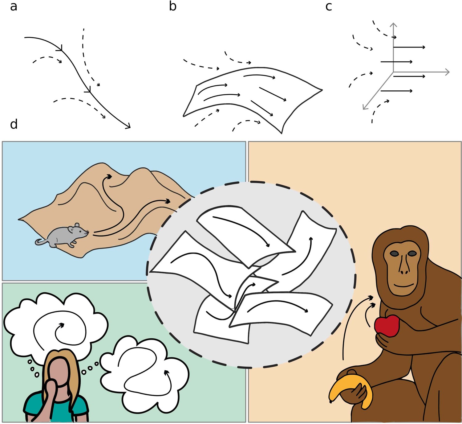
Schematic illustration of dynamic continuous attractors as a basis of different neural processes.
Top row: a scheme of continuous attractive manifolds, with a dynamic component in 1D (a), 2D (b) and 3D (c). The neural activity quickly converges on the attractive manifold (dotted arrows), then slides along it (full arrows), producing a dynamics that is temporally structured and constrained to a low dimensional subspace. Bottom row: multiple dynamic memories could be useful for route planning (top left), involved in mind wandering activity (bottom left) or represent multiple learned motor programs (right).
Figure 2
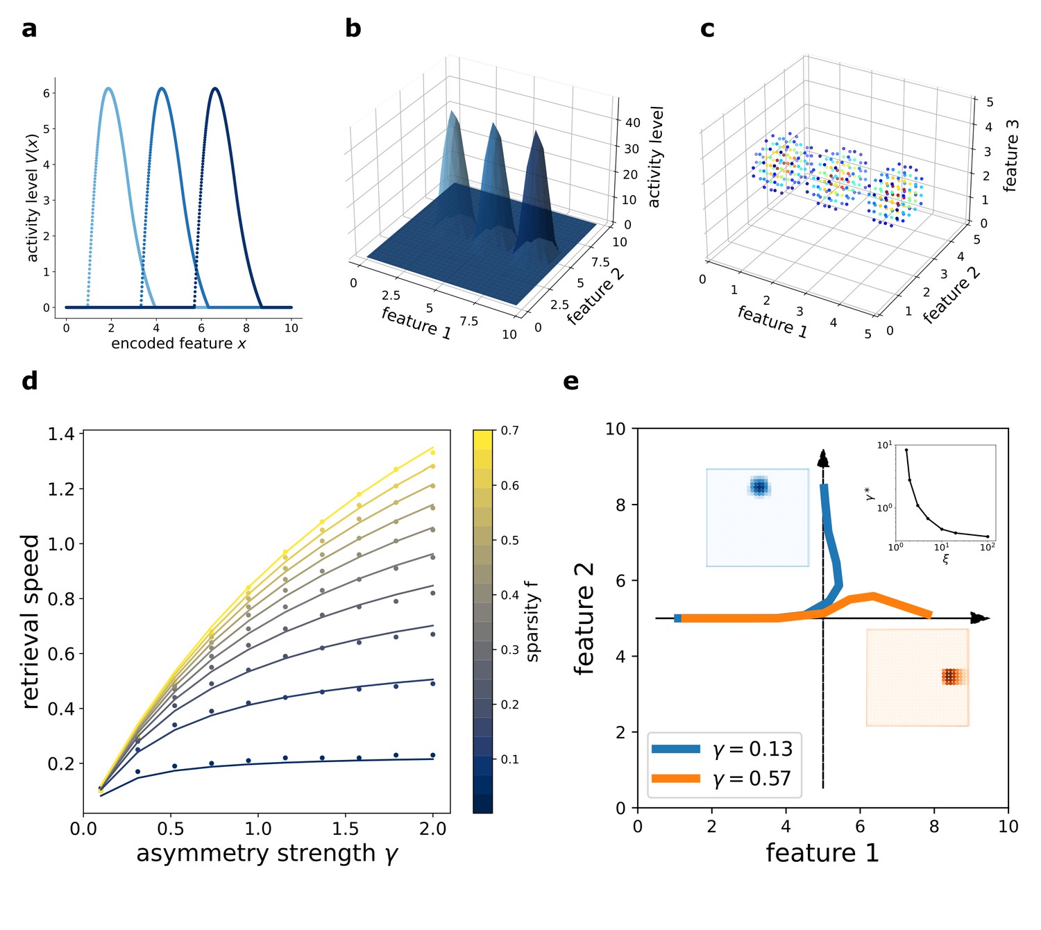
Dynamic retrieval of a continuous manifold.
First row: each plot presents three snapshots of the network activity at three different times (t1, t2 and t3), for a system encoding a one dimensional (a), two dimensional (b) and three dimensional (c) manifold. In (c), activity is color-coded (blue represents low activity, red is high activity, silent neurons are not plotted for better readability). In all cases, the anti-symmetric component is oriented along the x axis. (d) Dependence of the speed on γ and . Dots are data from numerical simulations, full lines are the fitted curves. (e) Retrieval of two crossing trajectories. Black arrows represent the two intersecting encoded trajectories, each parallel to one of the axis. Full colored lines show the trajectories actually followed by the center of mass of the activity from the same starting point. Blue curve: low γ, the activity switches trajectories when it reaches the crossing point. Orange curve: high γ, successful crossing. In both cases . The blue and the orange insets show the activity bumps in the corresponding cases; the top-right inset shows the dependence of the value , required for crossing, on ξ.
Figure 3
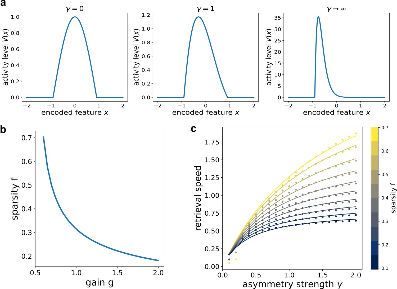
Analytical solution of the model.
(a) The shape of the bump for increasing values of γ. (b) Dependence of the sparsity on the gain of the network. (c) Dependence of the speed of the shift on γ, at different values of sparsity. Dots show the numerical solution (note some numerical instability at low and γ), full curves are the best fits.
Figure 4
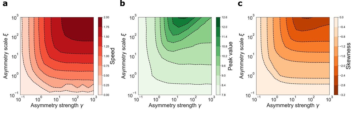
Dynamical retrieval in a wide range of parameters.
Effect of the kernel strength γ and its spatial scale ξ, in the case of the exponential kernel .(a) Retrieval speed (b) Peak value of the activity (c) Skewness of the activity bump.
Figure 5
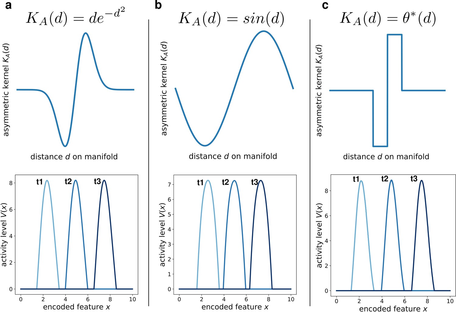
Different interaction kernels produce similar behavior.
Three examples of dynamics with the same symmetric component and three different anti-symmetric components. Top row: shape of the anti-symmetric component . Bottom row: three snapshots of the retrieval dynamics for the corresponding . (a) Gaussian derivative; (b) Sinusoidal; (c) Anti-symmetric step function, .
Figure 6
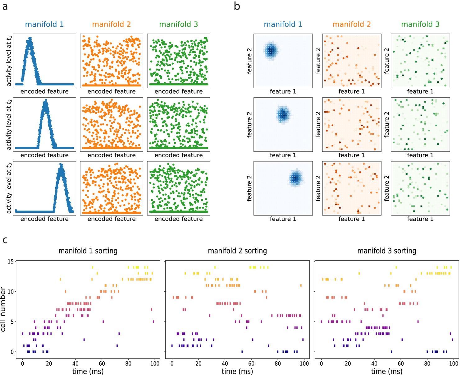
Dynamic retrieval in the presence of multiple memories.
(a) In one dimension (b) In two dimensions. Each row represents a snapshot of the dynamics at a point in time. The activity is projected on each of the three attractors stored in the network. In both cases, the first attractor is retrieved, and the activity organizes in a coherent bump that shifts in time. The same activity, projected onto the two non-retrieved maps looks like incoherent noise ((a) and (b), second and third columns). (c) Spiking patterns from a simulated recording of a subset of 15 cells in the network. When cells are sorted according to their firing field on the retrieved manifold (first column), they show sequential activity. The same activity is scattered if looked from the point of view of the unretrieved manifolds (second and third columns).
Figure 7
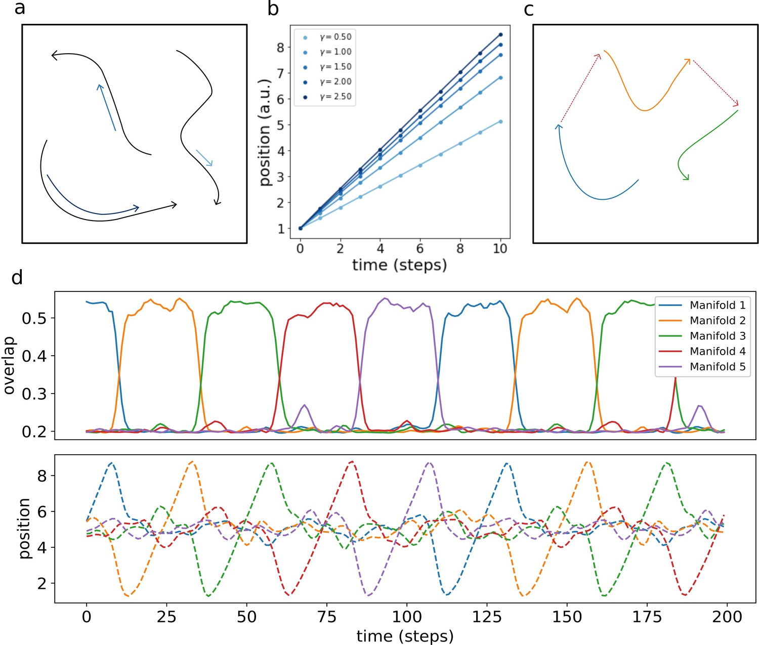
Retrieval speed and memory interactions.
(a) Multiple mainfolds with different velocity can be stored in a network with manifold-dependent asymmetric connectivity (b) The retrieved position at different timesteps during the retrieval dynamics of five different manifolds, stored in the same network, each with a different value of γ. (c) Manifolds memorized in the same network can be linked together (d) Sequential retrieval of five manifolds. Top row: overlap, measuring the overall coherence with the manifold, as a function of time. Bottom row: retrieved position in each manifold as a function of time.
Figure 8
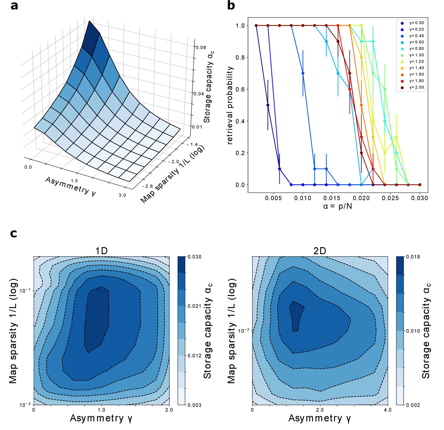
Storage capacity.
(a) Storage capacity of a diluted network: dependence on γ and (represented as ). (b) Storage capacity of a fully connected network: non monotonic dependence of the capacity on γ. Retrieval / no retrieval phase transition for different values of γ, obtained from simulations with , and , for 1D manifolds. Error bars show the standard error of the observed proportion of successful retrievals. The non-monotonic dependence of the capacity from γ can be appreciated here: the transition point moves toward the right with increasing γ up to , then back to the left. (c) Storage capacity of a fully connected network as a function of map sparsity and asymmetry strength γ, for a one-dimensional and a two-dimensional dynamic continuous attractor.
Appendix 1—figure 1
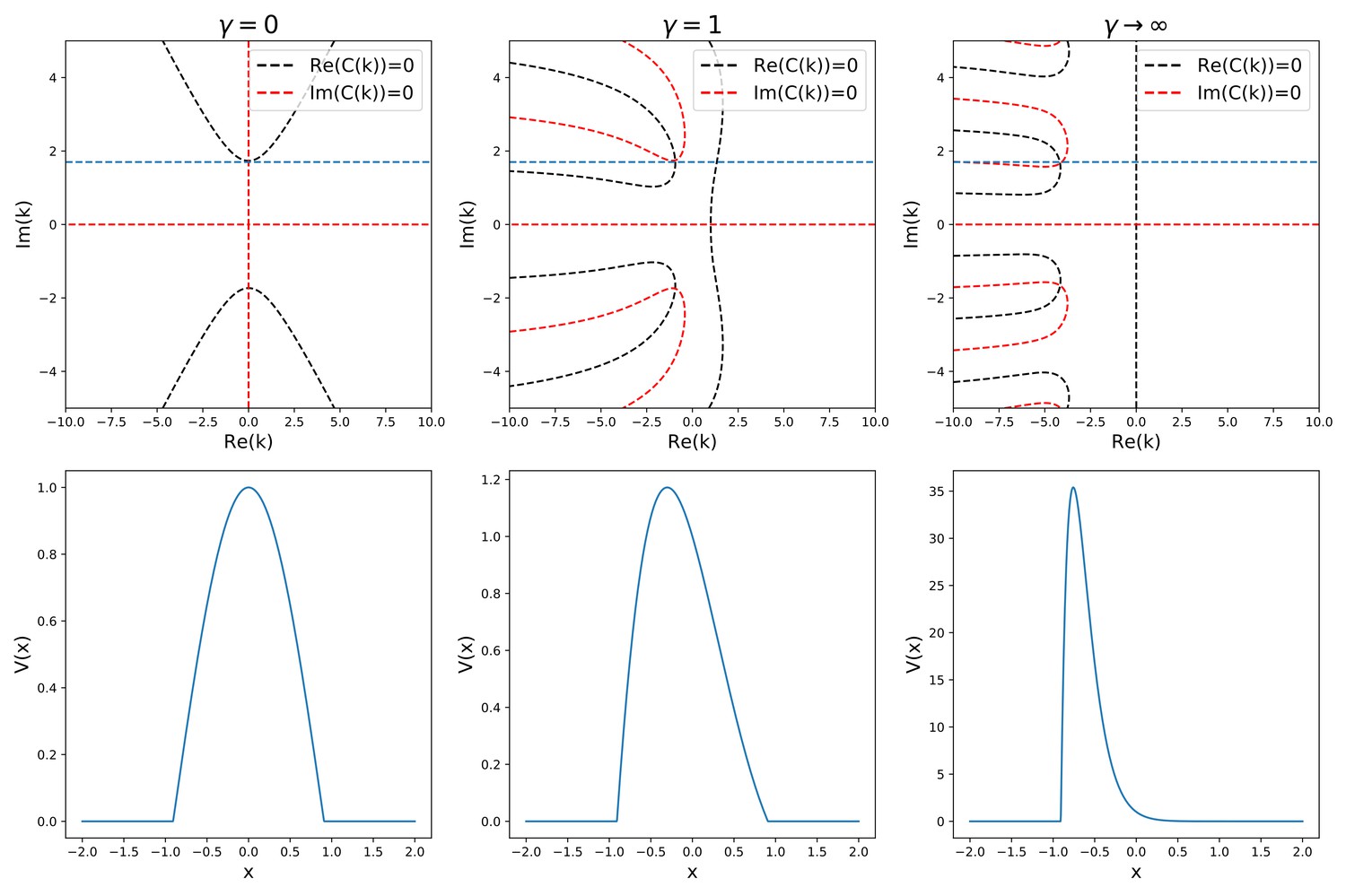
Analytic solution of Equation (38).
The top row shows the graphical procedure to find the complex zeros of the characteristic given in (40), for three different values of γ. Black and red lines show the zeros of the real and imaginary part of , respectively. Their intersections are the complex solutions to . The blue line represents the sparsity constraint . The bottom row shows the corresponding solution shapes.
Appendix 1—figure 2

Solutions to Equation 52 for , , , .
Then, keeping u0 fixed, we can repeat a similar procedure to find for different values of γ. Also in this case, the solution either diverges or oscillates, apart from a single value , for which the solution has the desired shape (see Appendix 1—figure 3). This eliminates the arbitrariness in the choice of since it imposes, for given and , a relation .
Appendix 1—figure 3
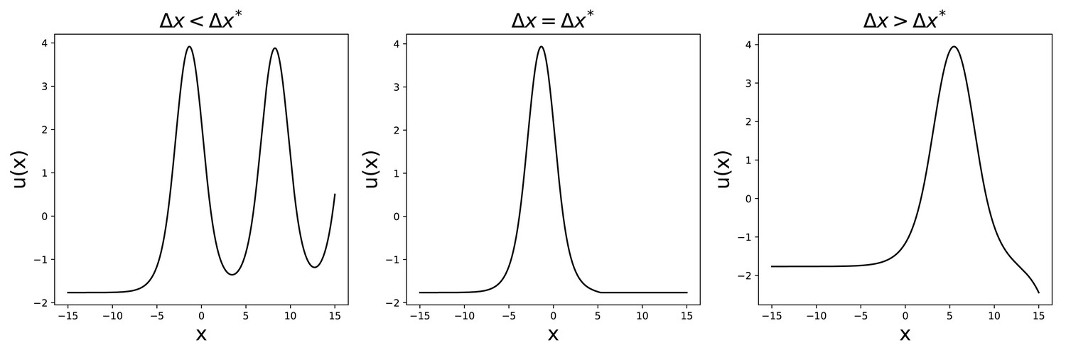
Solutions to Equation 52 for , , .
We can then find the shape of the bump for given values of , + and γ, from which we can obtain the profile that we need for the calculation of the storage capacity. Some examples of the obtained profiles, for different values of γ, are shown in Appendix 1—figure 4.
Appendix 1—figure 4

Activity profile , obtained for the same and , at different values of γ.
Plugging the obtained form of into Equation 29, we can calculate the capacity. The dependence of the capacity on γ is shown, for , in Appendix 1—figure 5.
Appendix 1—figure 5
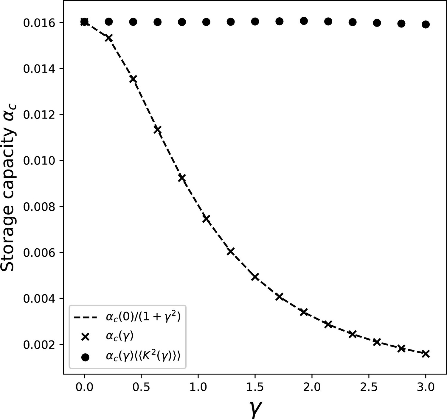
Dependence of the storage capacity on γ, for .
The crosses show the full solution of Equations 27 and 29. The dashed line is obtained by taking the value of the capacity obtained with full solution at , and multiplying it by the scaling of the kernel variance . Full dots show the value of capacity obtained with the full solution and the contribution of the kernel variance factored out.
Additional files
Download links
A two-part list of links to download the article, or parts of the article, in various formats.
Downloads (link to download the article as PDF)
Open citations (links to open the citations from this article in various online reference manager services)
Cite this article (links to download the citations from this article in formats compatible with various reference manager tools)
Continuous attractors for dynamic memories
eLife 10:e69499.
https://doi.org/10.7554/eLife.69499


