The nematode worm C. elegans chooses between bacterial foods as if maximizing economic utility
- Institute of Neuroscience, University of Oregon, United States
- Center for Neural Science, New York University, United States
- Neuroscience Institute, New York University School of Medicine, United States
- Department of Economics, University of Oregon, United States
- Department of Neuroscience, Pomona College, United States
- Department of Chemistry, Pomona College, United States
- Picower Institute for Learning and Memory, Department of Brain & Cognitive Sciences, Massachusetts Institute of Technology, United States
- Department of Economics, University of California, San Diego, United States
Figures
Figure 1
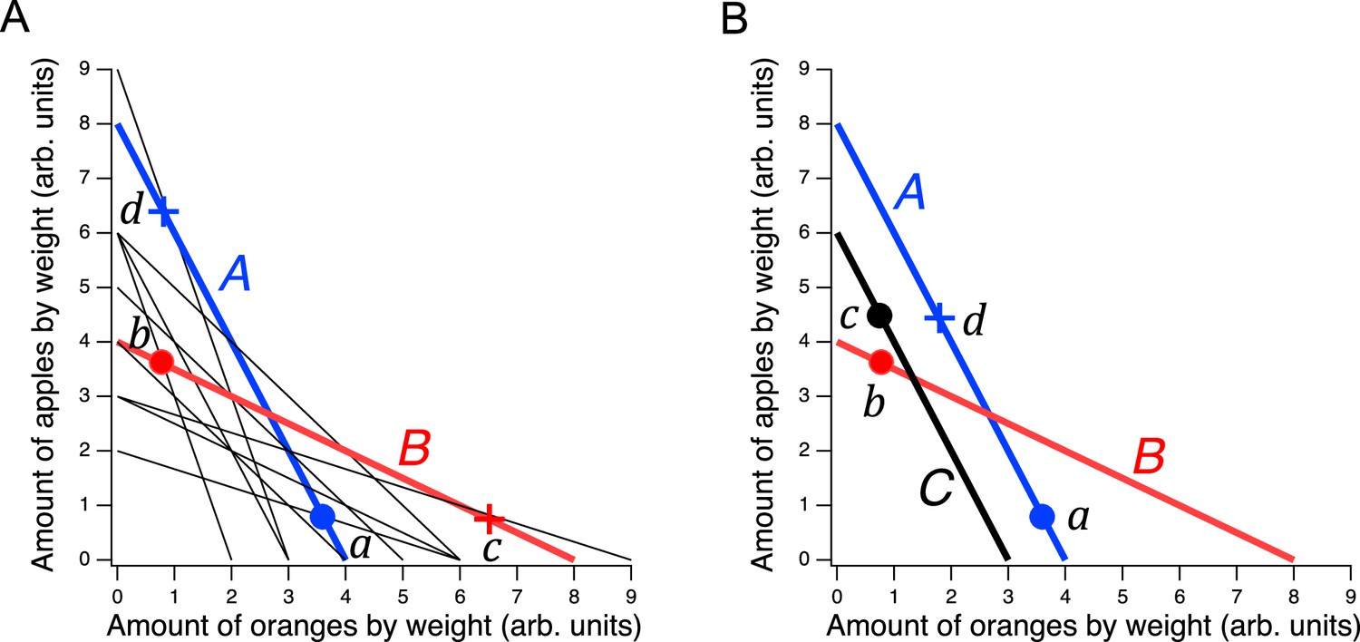
Design of a GARP experiment and tests for utility maximization.
(A) Direct violation of utility maximization. Diagonal lines indicate choice sets (=11). Choice sets are distinguished by having different values of the overall budget and/or different prices for at least one of the goods. Within a choice set, the expenditure implied by each bundle of goods is constant and equals the budget. In A (blue), the budget is $8, oranges are $2 per unit, apples are $1 per unit. In B (red): the budget is $8, oranges are $1 per unit, apples are $2 per unit. Filled circles, chosen amounts; plus signs, available amounts not chosen. Given the choices shown and the more is better rule, and . Therefore, choices and directly violate utility maximization. (B). Indirect violation of utility maximization. Symbols as in A. The choices and constitute an indirect violation of utility maximization as described in the text.
Figure 2 with 2 supplements

Edible bacteria act as goods over which worms form preferences through experience.
(A) Food quality training and preference assays. Filled circles represent patches of bacteria as indicated in the key. Stars indicate worm starting locations. (B). Mean preference at 60 min. in the open-field accumulation assay for trained and untrained N2 and ceh-36 mutants. Asterisk, see Table 21. Replicates, Trained, strain(): N2(8), ceh-36(9). Replicates, Untrained, strain(): N2(8), ceh-36(8). (C). Mean preference vs. time for trained and untrained N2 worms in T-maze accumulation assays, with and without sodium azide in the food patches. (D). Mean preference index vs. time for trained and untrained cat-2(tm2261) mutants and N2 controls in T-maze accumulation assays. N2 data are from C. (B–D). Error bars, 95% CI. For sample size (N), statistical methods used, and significance level, see Table 2, rows 1-15.
-
Figure 2—source data 1
Edible bacteria act as goods over which worms form preferences through experience.
- https://cdn.elifesciences.org/articles/69779/elife-69779-fig2-data1-v2.xlsx
-
Figure 2—source data 2
Loss of dopamine signaling does not reduce proportion of time on food.
- https://cdn.elifesciences.org/articles/69779/elife-69779-fig2-data2-v2.xlsx
Figure 2—figure supplement 1
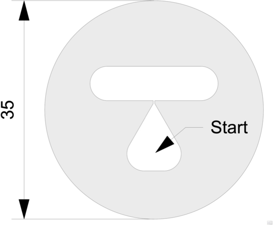
T-maze diagram.
The teardrop shaped feature acts as worm diode. Worms leave the teardrop more easily than they re-enter it, thus helping to ensure they do not congregate at the starting point. The mask’s ability to confine worms in the test area is improved by floating the maze on the surface of the agarose medium while it is still liquid (M. Brooks, pers. comm.). Dimensions are in mm.
Figure 2—figure supplement 2

Loss of dopamine signaling does not reduce proportion of time on food.
Mutations in the gene cat-2 do not significantly later the ability of worms to find and remain in food patches. Statistics (t-tests): N2 vs. cat-2(n4547), t(38) = –0.95, p=0.35; N2 vs cat-2(e1112), t(40) = –1.38, p=0.18. N2, n = 30; cat-2(n4547), n = 10; cat-2(e1112) n = 12. Error bars, SEM.
Figure 3
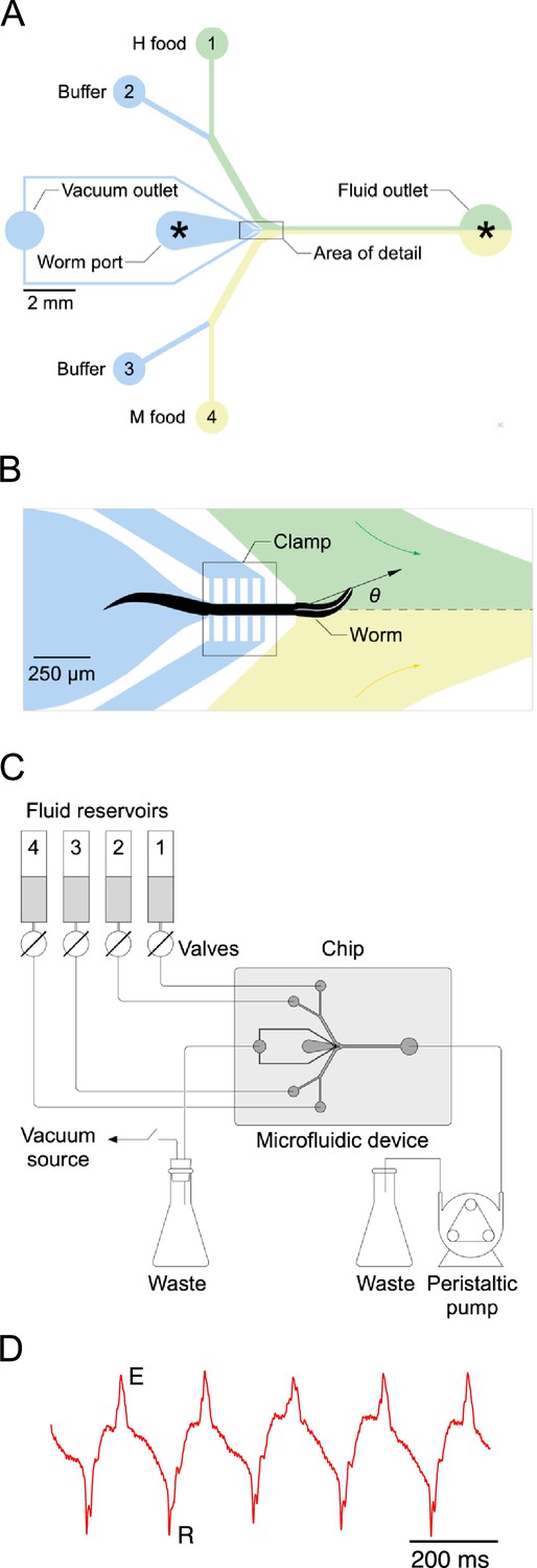
Single-worm food choice assays.
(A) Layout of the Y-chip. Asterisks indicate the position of recording electrodes. Ground electrodes (not shown) were inserted into the food and buffer ports to reduce electrical interference. The chip is shown configured for the experiments in Figures 4B and 5B. (B). Area of detail shown in A. The dashed line is the centerline of chip; the white line within the worm is its centerline. The black arrow connects the middle of the neck where it enters the food channel with anterior end of worm’s centerline. Positive values of head angle () indicate displacement toward H food. Colored arrows show direction of flow. (C). Schematic overview of fluidic system. (D). Typical electropharyngeogram. Each pair of excitation (E) and relaxation (R) spikes constitutes one pharyngeal pump.
Figure 4
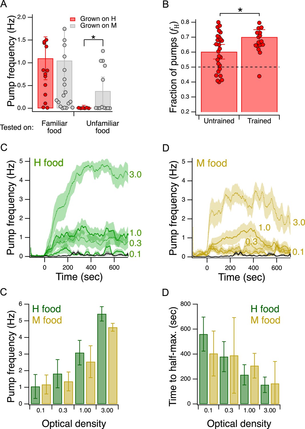
Validation of the Y-chip for measuring food preferences.
(A) Familiar food effect. Mean pump frequency of worms grown on H or M food and tested on the same or the converse food. Asterisk, see Table 217. Both foods were at OD 1. Pumping was recorded for 12 min. Replicates, Grown on H, tested on (): Familiar(16), Unfamiliar(6). Replicates, Grown on M, tested on(): Familiar(23), Unfamiliar(13). Error bars, 95% CI. (B). Food quality learning. Mean fraction of pumps in H food in trained and untrained worms. Asterisk, see Table 220. The dashed line indicates equal preference for H and M food. Both foods were at OD 1. Error bars, 95% CI. (C,D). Time course of pump frequency at four different densities of familiar food. Food enters the chip at sec. Optical density is indicated next to each trace. The black trace shows pumping in the absence of food. Shading, ± SEM E. Dependence of mean peak pump frequency density of familiar food. (F). Dependence of latency to half-maximal pump frequency on density of familiar food. (E,F). Error bars, 95% CI. For sample size (N), statistical methods used, and significance level, see Table 2, rows 16-000.
-
Figure 4—source data 1
Validation of the Y-chip for measuring food preferences.
- https://cdn.elifesciences.org/articles/69779/elife-69779-fig4-data1-v2.xlsx
Figure 5 with 2 supplements
Economic analysis of food choice in C. elegans.
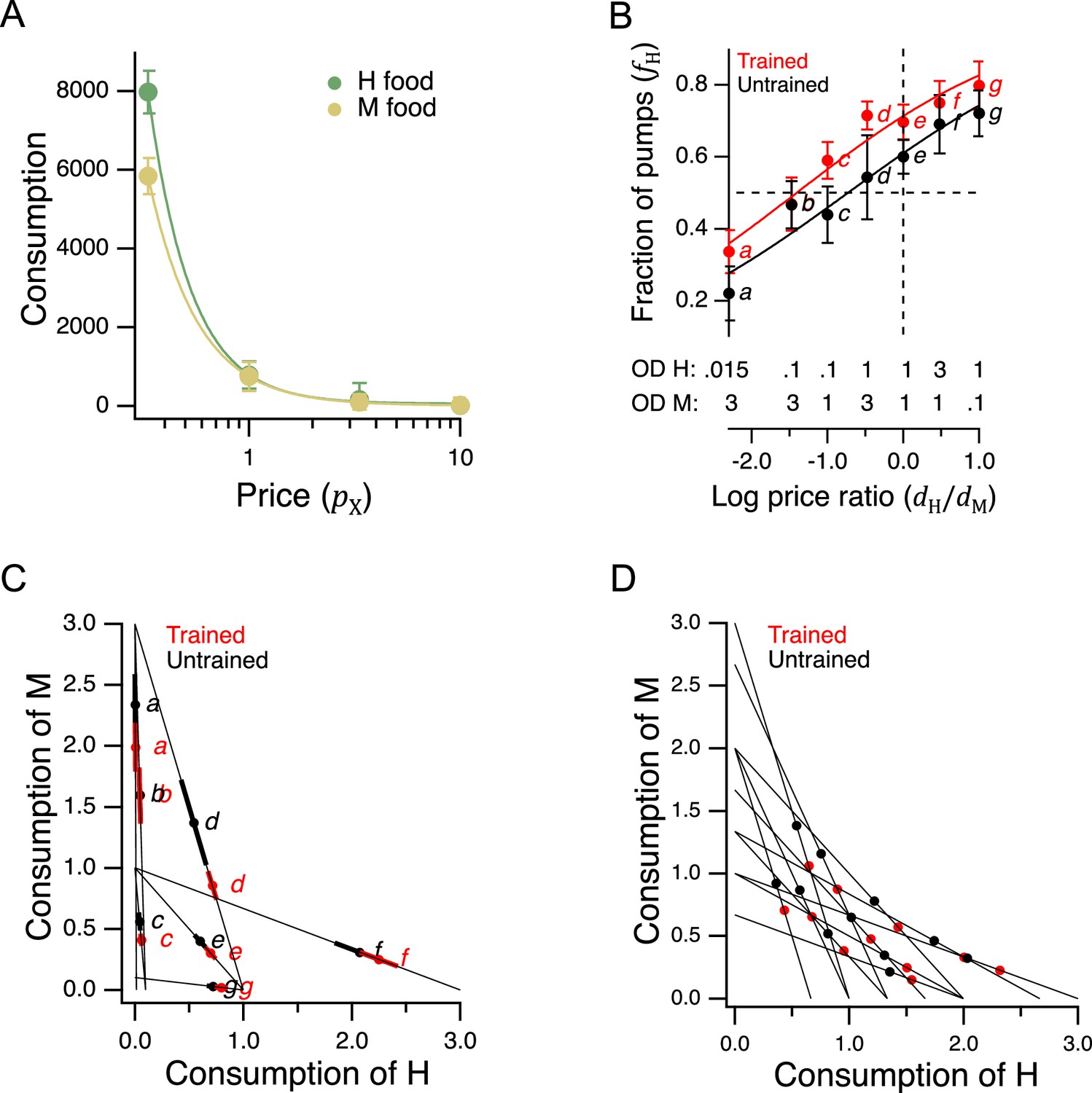
(A) Demand curves. Mean consumption of familiar food versus its price. Consumption is computed as number of pumps times optical density of bacteria. Price is computed by Equation 2. The data are fit by Equation 8 with for H food and for M food. H food price(): 0.33(13), 1.0 (16), 3.3 (21), 10(15). M food price(): 0.33(9), 1.0 (23), 3.3 (7), 10(10). (B). Price ratio curves. Food preference, measured as fraction of pumps in H food, versus price ratio for Trained and Untrained worms. Horizontal dashed line: indifference between H and M food; vertical dashed line: H and M food at equal price. Data at log price ratio = 0 are replotted from Figure 4B. Replicates, Trained, point(): a(9), b(14), c(18), d(27), e(20), f(10), g(6). Replicates, Untrained, point(): a(12), b(17), c(13), d(12), e(28), f(10), g(7). (C). GARP analysis of C. elegans food preferences. Plotted points show mean consumption of M food versus consumption of H food in Trained and Untrained worms. Lines are choice sets as in Figure 1. The and intercepts of each line indicate the amounts of H and M food that would have been consumed if the worm spent all its pumps on one or the other food type. Error bars, 95% CI. (D). Predicted consumption of H and M food in Trained and Untrained animals on a widely-used ensemble containing 11 budget lines (Harbaugh et al., 2001). (A–C). Error bars, 95% CI. For sample size (N), statistical methods used, and significance level, see Table 2, rows 23-26.
-
Figure 5—source data 1
Economic analysis of food choice in C. elegans.
- https://cdn.elifesciences.org/articles/69779/elife-69779-fig5-data1-v2.xlsx
-
Figure 5—source data 2
Distributions of preference values in trained and untrained animals in Figure 5B.
- https://cdn.elifesciences.org/articles/69779/elife-69779-fig5-data2-v2.xlsx
Figure 5—figure supplement 1
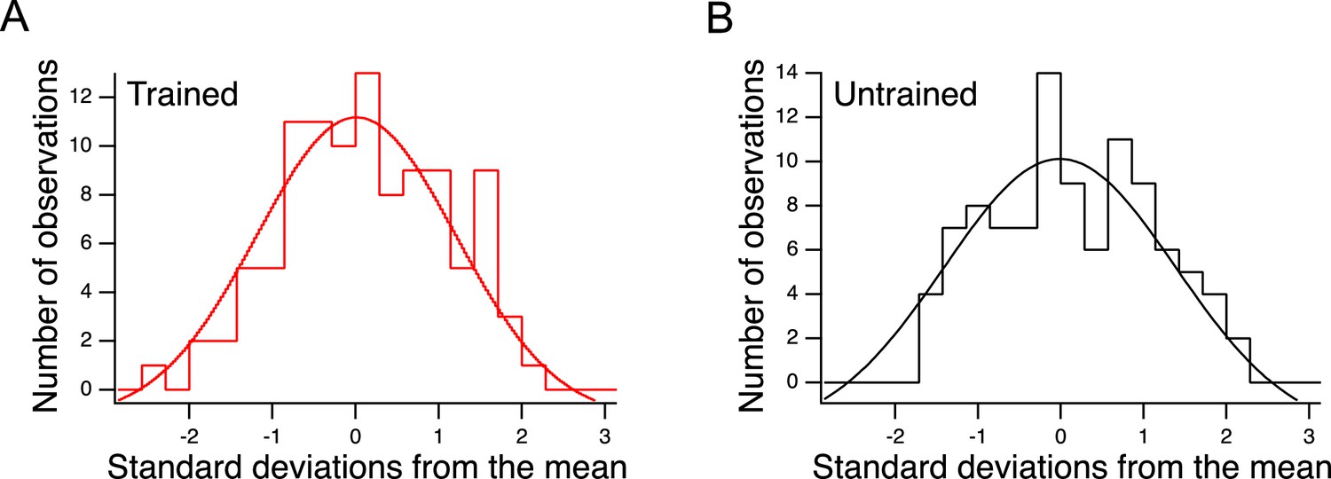
Distributions of preference values in trained and untrained animals in Figure 5B.
Figure 5—figure supplement 2

Indirectly revealed preferences inherent in the choices shown in Figure 5C.
Figure 6
Higher order features of utility maximization.
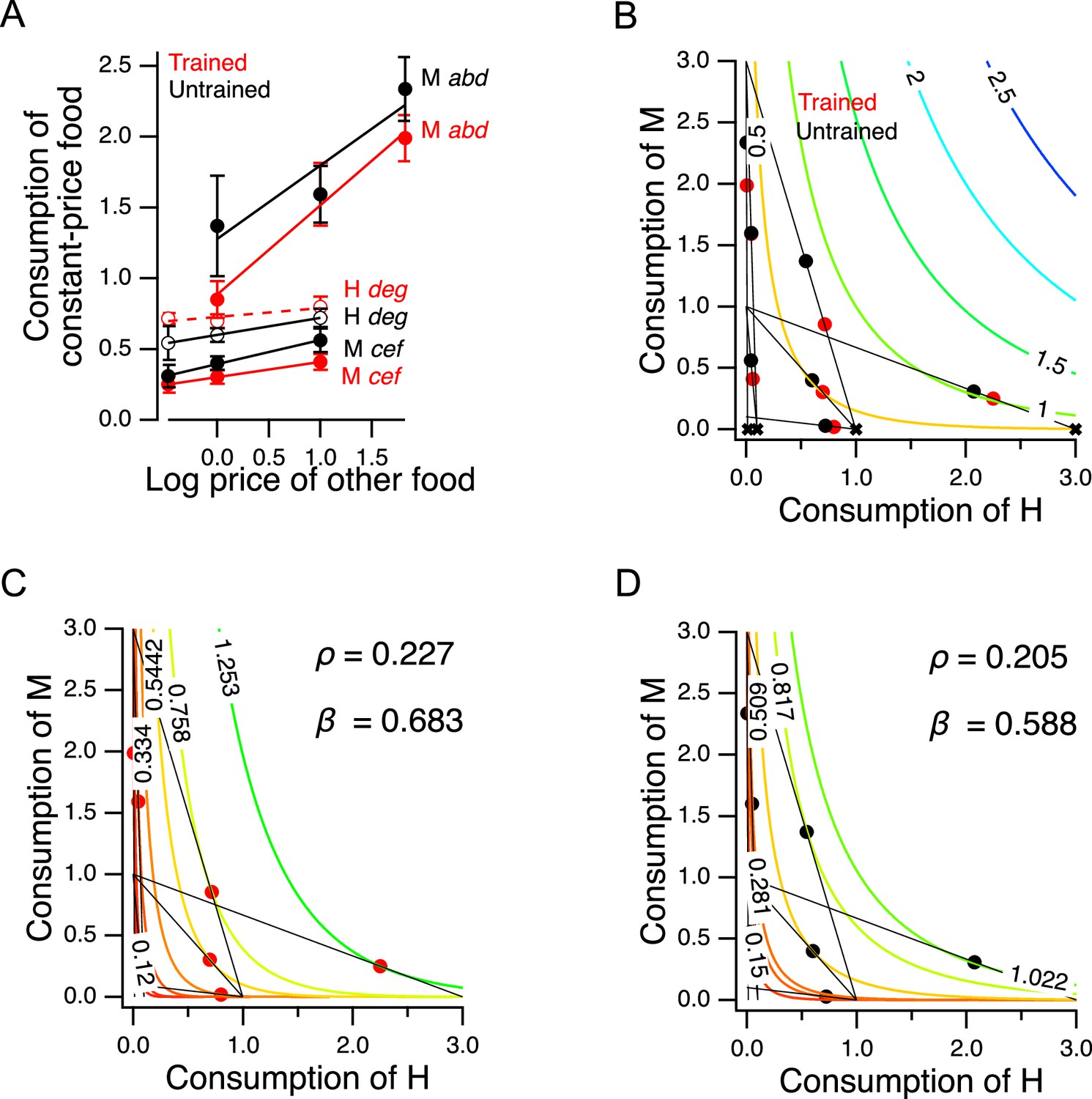
(A) H and M food act as substitutes. Consumption is plotted against price for triplets of cost ratios in which the concentration of one food was constant and the concentration of the other food was variable (see Supplementary file 1). Lower case italic letters: data points in Figure 5B. Capital letters: the food whose density was constant, the consumption of which is plotted on the -axis. Solid lines: regression slope different from zero (); dashed lines: slope not different from zero. Error bars, 95% CI. (B). H and M food are not perfect substitutes. Colored contour lines are indifference curves in a perfect substitute model (Equation 10) with . Data points from Figure 5C are replotted for comparison, with associated budget lines, according to the conventions of that figure. ‘X’ symbols indicate the point of highest utility on each budget line. (C–D). Best fitting parameterizations of the CES function (Equation 11) for Trained and Untrained animals. Each panel shows the seven the iso-utility lines that are tangent to the budget lines. Goodness of fit can be assessed by observing that the iso-utility lines are tangent to the budget lines at, or near, the data points which indicate mean consumption of H and M food. For sample size (N), statistical methods used, and significance level, see Table 2, rows 27-32.
-
Figure 6—source data 1
Higher order features of utility maximization.
- https://cdn.elifesciences.org/articles/69779/elife-69779-fig6-data1-v2.xlsx
Figure 7
Behavioral mechanisms of utility maximization.
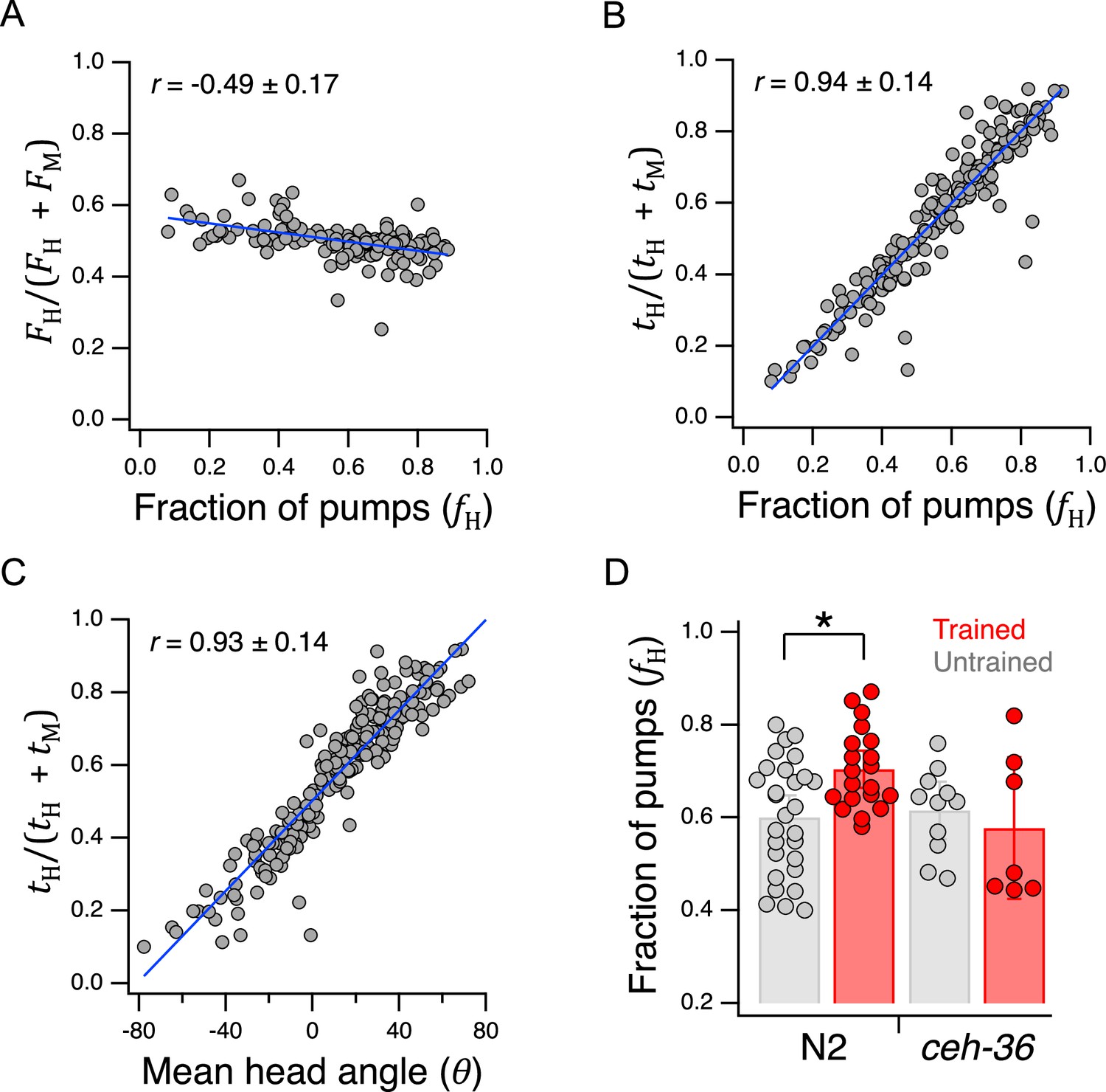
(A) Pumping-rate model of preference. Equation 13 is evaluated for each worm in Figure 5B and the result is plotted against preference in terms of fraction of pumps in H food for the same animal. (B). Dwell-time model of preference. Same as A but using Equation 14. (C). Regression of Equation 14 against mean head angle as defined in Figure 3B. (A–C). Blue lines: regressions on the data. (D). Diminished ceh-36 function eliminates the effect of food quality training on food preference. Asterisk, see Table 238. (H and M) are at OD = 1. N2 data are from Figure 4B. Replicates, Trained, strain(): N2(20), ceh-36(7). Replicates, Untrained, strain(): N2(28), ceh-36(11). Error bars, 95% CI. Correlation coefficients are shown ±95% CI. For sample size (N), statistical methods used, and significance level, see Table 2, rows 33-39.
-
Figure 7—source data 1
Behavioral mechanisms of utility maximization.
- https://cdn.elifesciences.org/articles/69779/elife-69779-fig7-data1-v2.xlsx
Figure 8 with 1 supplement
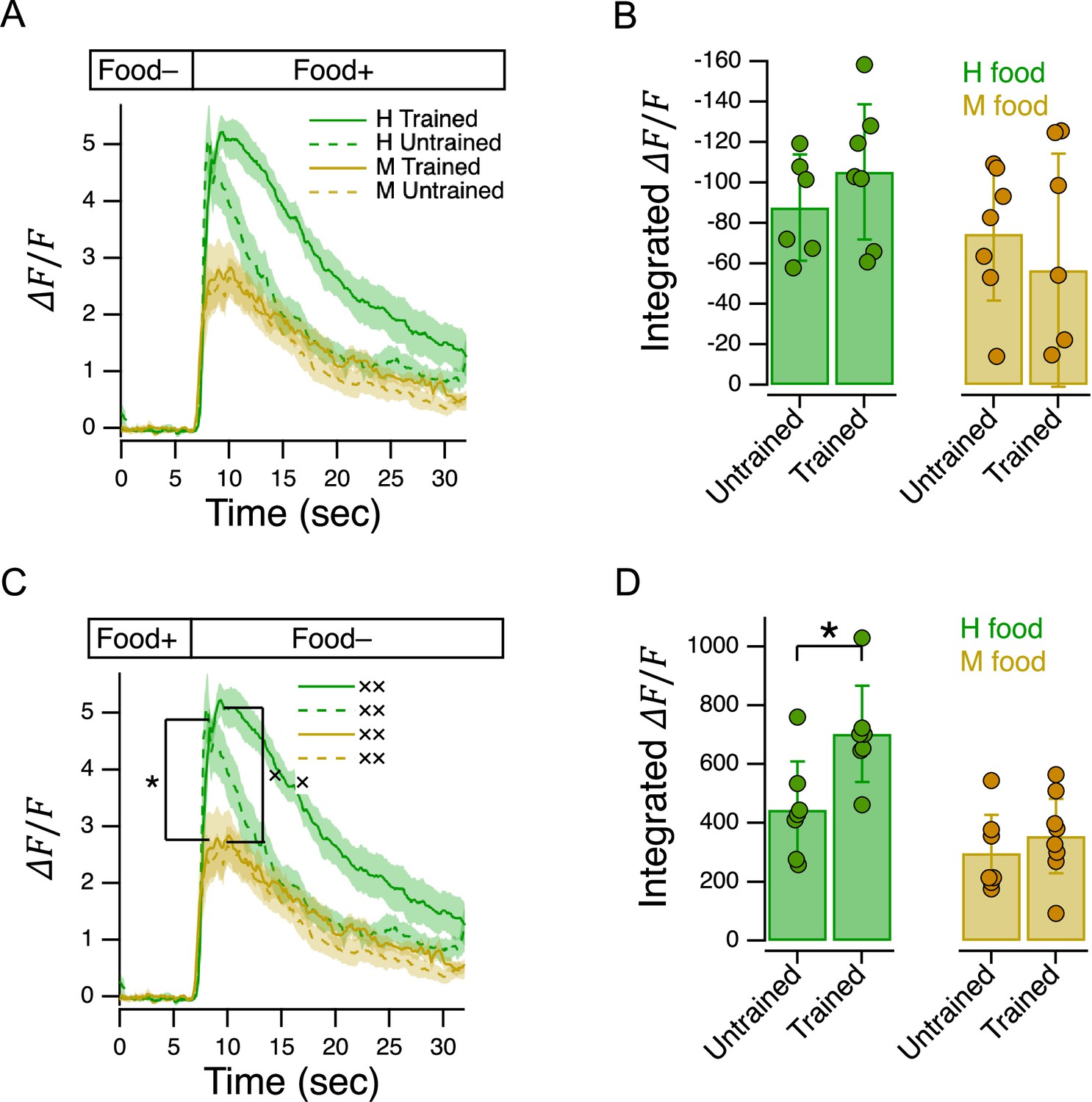
Characterization of AWC’s response to delivery and removal of food.
(A) Ensemble averages of relative fluorescence versus time in response to onset of the indicated food in trained and untrained animals. (B). Summary of data in A, showing mean integrated calcium transients. (C). Ensemble averages of relative fluorescence versus time in response to removal of the indicated food in trained and untrained animals. Asterisk: untrained group, mean peak response, H vs. M food, see Table 242. Cross: trained group, mean peak response, H vs. M food, see Table 243. (D). Summary of data in C, showing mean integrated calcium transients Asterisk, see Table 246. (A–D). OD = 1 for H and M food. Shading, ± SEM. Error bars, 95% CI. For sample size (N), statistical methods used, and significance level, see Table 2, rows 40-47.
-
Figure 8—source data 1
Characterization of AWC's response to delivery and removal of food.
- https://cdn.elifesciences.org/articles/69779/elife-69779-fig8-data1-v2.xlsx
Figure 8—figure supplement 1
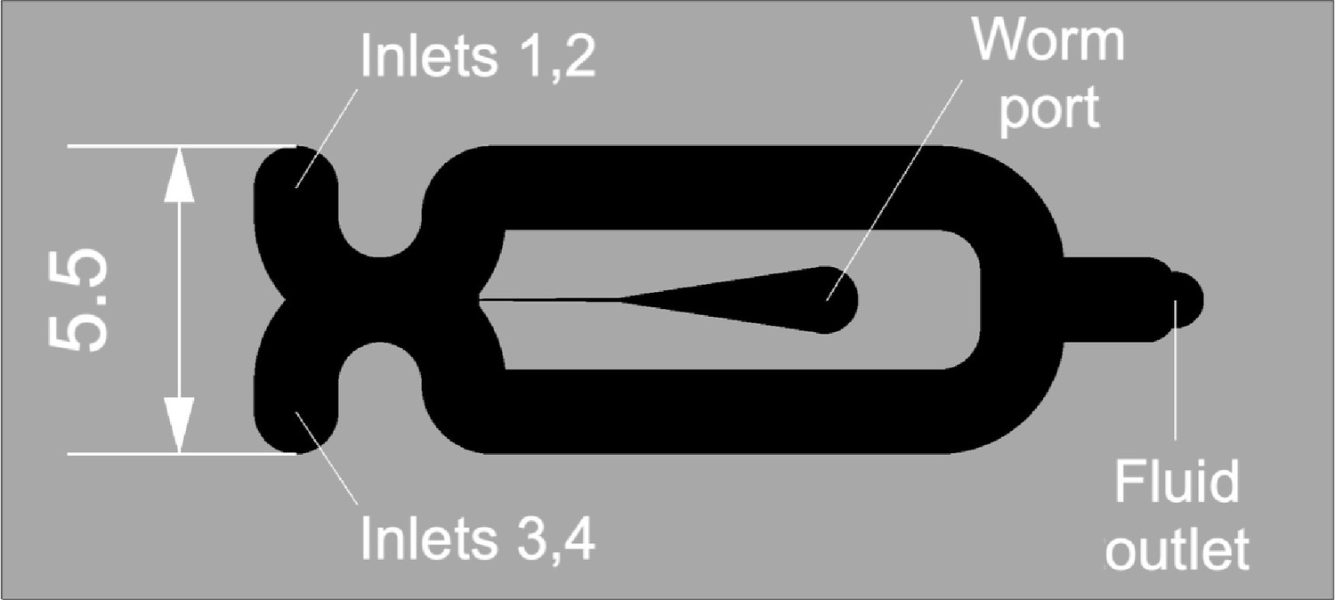
Imaging chip.
Fluidic features are shown in black. Dimensions are in mm.
Figure 9 with 1 supplement
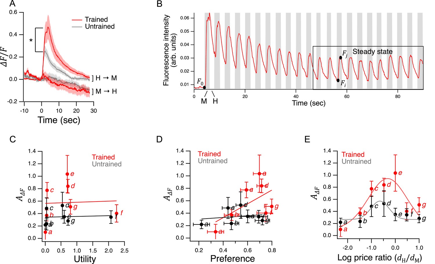
Characterization of AWC’s response to bacterial foods in Y-chip assays.
(A) Ensemble average of relative fluorescence versus time in response to transitions from H to M (H→M) or M to H (M→H) food. Asterisk, see Table 248. Both foods were presented at OD = 1. Food was switched at = 0. H→M, Trained, = 16; H→M, Untrained = 14. M→H, Trained, = 16; M→H, Untrained, = 15. Shading,±SEM. (B). Typical fluorescence waveform in response to a series of transitions between H and M food. Notation: , baseline fluorescence after sustained exposure to H food (≅ 2 min.); , maximum H→M fluorescence; , minimum M→H fluorescence. The box delineates the time period of presumptive steady-state responses over which mean response amplitudes were computed for each recorded worm. (C–E). versus utility, preference, and log price ratio. Lines and curves are, respectively, linear and gaussian fits. Italic letters refer to labeled points in Figure 5B. Replicates, Trained, point(): a(6), b(10), c(18), d(12), e(19), f(10), g(9). Replicates, Untrained. point(): a(8), b(11), c(10), d(8), e(12), f(8), g(10). Error bars, 95% CI. For sample size (N), statistical methods used, and significance level, see Table 2, rows 48-55.
-
Figure 9—source data 1
Characterization of AWC’s response to bacterial foods in Y-chip assays.
- https://cdn.elifesciences.org/articles/69779/elife-69779-fig9-data1-v2.xlsx
Figure 9—figure supplement 1
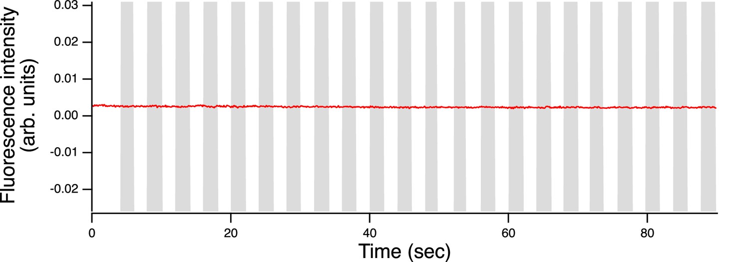
Control for mechanical artifacts in the experiment of Figure 9B assays.
This trace shows a typical AWC fluorescence waveform in response to a series of mock transitions between H and M food in which all syringes in the imaging system contained food-free buffer.
Figure 10
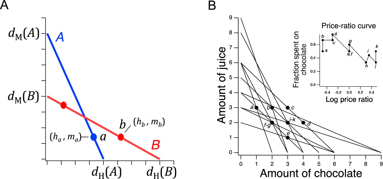
Price ratio curves and utility maximization.
(A) A pair of intersecting budget lines wherein choices a and b are governed by a price-ratio curve (not shown) that is monotonic-increasing. To support a direct violation of GARP, a must be to the right of the intersection of lines A and B, and b must be to the left of it. However, by price-ratio monotonicity, b must lie to the right of a, for reasons described in the text. This constraint precludes direct violations of GARP. (B). Choice data from a human participant in a GARP experiment (Camille et al., 2011). The data are consistent with utility maximization. Inset, price ratio data inferred from the experiment. Log price ratios for points a-k are calculated as , where and are, respectively, the and intercepts of budget line . The fraction of total budget spent on good X is computed as , where is the amount of good X chosen on line .
Videos
Video 1
Foraging behavior in the Y-chip.
Simulated Y-chip experiment. The worm is held at its midsection by a vacuum activated clamp, leaving the head (left) and tail free to move. The both fluid streams contain bacteria-free buffer, flowing to the right to left. Food dye was added to the lower stream to visualize the interface between streams. Bubbles originating at the clamp are formed by air that has been pulled through the PDMS walls of the chip by the vacuum. The worm prefers the dyed stream as it contains potassium sorbate, which acts as a chemoattractant.
Tables
Table 1
Volatile organic compounds released by H and M food.
| Designation | CAS# | Compound | H food (DA1877) | M food (DA1885) |
|---|---|---|---|---|
| a | 1534-08-3 | Methylthioacetate* | 0.0 | 1.0 |
| b | 624-92-0 | Dimethyl disulfide* | 19.4 | 38.3 |
| c | 2432-51-1 | S-Methyl butanethioate† | 0.0 | 4.7 |
| d | 23747-45-7 | S-Methyl 3-methylbutanethioate | 0.0 | 2.4 |
| e | 3658-80-8 | Dimethyltrisulfide* | 1.5 | 6.4 |
-
Compounds were identified by gas chromatography-mass spectrometry of headspace of H and M food and confirmed with known standards. Amounts were inferred from the area under elution peaks, averaged across two replicates, and normalized to the amount of methylthioacetate in DA1885.
-
*
Identified chemoattractant; other compounds are uncharacterized in chemotaxis assays.
-
†
Vapor is nematicidal.
Table 2
Statistics.
Horizontal location of cell entries varies by row.
| Row | Figure | Test | Effect or comparison tested | Units of replication or sampling | Number of replicates or samples | Statistic | DF 1 or combined DF | DF 2 | p | Effect size | |
|---|---|---|---|---|---|---|---|---|---|---|---|
| 1 | 2B* | t-test | Trained N2 vs. Untrained N2 | Assay plates | N=8 | t | 2.50 | 14 | – | 2.56E-02 | 1.248 |
| 2 | 2B | t-test | N2 Untrained, 60 min mean I>0 | Assay plates | N=8 | t | 10.22 | 7 | – | 1.86E-05 | – |
| 3 | 2B | t-test | ceh-36 Untrained, 60 min mean I>0 | Assay plates | N=8 | t | 3.58 | 7 | – | 9.01E-03 | – |
| 4 | 2B | t-test | Trained ceh-36 vs. Untrained N2 | Assay plates | N=8 | t | 0.64 | 14 | – | 2.50E-01 | – |
| 5 | 2B | t-test | Untrained ceh-36 vs. Untrained N2 | Assay plates | N=8 | t | 1.87 | 14 | – | 8.22E-02 | – |
| 6 | 2B | t-test | Trained ceh-36 vs. Untrained ceh-36 | Assay plates | N=8 | t | 0.90 | 14 | – | 3.82E-01 | – |
| 7 | 2C | Two-factor ANOVA, repeated measures, main effect | Azide- Trained vs. Azide- Untrained | Assay plates | N≥9 / treatment | F | 11.28 | 1 | 21 | 2.98E-03 | 0.349 |
| 8 | 2C | t-test | Azide +Trained, 60 min mean I>0 | Assay plates | N=10 | t | 6.35 | 10 | – | 8.36E-05 | – |
| 9 | 2C | t-test | Azide+, Untrained, 60 min mean I>0 | Assay plates | N=10 | t | 3.09 | 10 | – | 1.15E-02 | – |
| 10 | 2C | Two-factor ANOVA, repeated measures, main effect | Azide +Trained vs. Azide +Untrained | Assay plates | N=10 / treatment | F | 10.32 | 1 | 20 | 4.37E-03 | 0.340 |
| 11 | 2C | Two-factor ANOVA, repeated measures, main effect | Azide +Trained, vs. Azide– Trained | Assay plates | N≥9 / treatment | F | 11.17 | 1 | 19 | 3.43E-03 | 0.370 |
| 12 | 2C | Two-factor ANOVA, repeated measures, main effect | Azide +Untrained vs. Azide– Untrained | Assay plates | N≥10 / treatment | F | 38.28 | 1 | 22 | 3.16E-06 | 0.635 |
| 13 | 2D | Two-factor ANOVA, repeated measures, main effect | Untrained N2 vs. Untrained cat-2 | Assay plates | N≥9 / strain | F | 23.25 | 1 | 21 | 9.14E-05 | 0.493 |
| 14 | 2D | Two-factor ANOVA, repeated measures, main effect | Trained N2 vs. Trained cat-2 | Assay plates | N=9 / strain | F | 52.50 | 1 | 18 | 9.74E-07 | 0.207 |
| 15 | 2D | Two-factor ANOVA, repeated measures, main effect | Trained cat-2 vs. Untrained cat-2 | Assay plates | N=9 / treatment | F | 0.90 | 1 | 18 | 6.43E-01 | – |
| 16 | 4A | Two-factor ANOVA, main effect | Familiar vs. Unfamiliar | Worms | N≥19 / treatment | F | 10.46 | 1 | 54 | 2.10E-03 | 0.162 |
| 17 | 4 A* | t-test | Unfamiliar, grown in H vs. grown in M | Worms | N≥6 | t | 2.65 | 17 | – | 2.10E-02 | 0.876 |
| 18 | 4B | t-test | Trained, f_H>0.5 | Worms | N=19 | t | 8.60 | 18 | – | 8.60E-08 | – |
| 19 | 4B | t-test | Untrained, f_H>0.5 | Worms | N=28 | t | 4.35 | 27 | – | 1.70E-04 | – |
| 20 | 4B* | t-test | Trained vs. Untrained | Worms | N≥19 | t | 2.95 | 44 | – | 5.11E-03 | 0.850 |
| 21 | 4E | Two-factor ANOVA | Main effect of optical density | Worms | N≥22 / density | F | 31.58 | 3 | 108 | 9.80E-15 | 0.467 |
| 22 | 4F | Two-factor ANOVA | Main effect of optical density | Worms | N≥22 / density | F | 3.10 | 3 | 106 | 3.00E-02 | 0.081 |
| 23 | 5B | Two-factor ANOVA | Main effect of price ratio | Worms | Avg N=15 / ratio | F | 44.13 | 6 | 195 | 7.89E-34 | 0.576 |
| 24 | 5B | Two-factor ANOVA | Main effect of training | Worms | Avg N=15 / ratio | F | 36.16 | 1 | 195 | 8.82E-09 | 0.156 |
| 25 | 5B | t-test | Trained, point a, mean f_H<0.5 | Worms | N=9 | t | 6.22 | 8 | – | 2.52E-04 | – |
| 26 | 5B | t-test | Untrained, point a, mean f_H<0.5 | Worms | N=12 | t | 8.29 | 11 | – | 4.66E-06 | – |
| 27 | 6A | Regression with replication slope test | Figure 6A, points abd, Trained slope ≠ 0 | Worms | N≥9 / ratio | F | 118.79 | 1 | 47 | 1.85E-14 | – |
| 28 | 6A | Regression with replication slope test | Figure 6A, points abd, Untrained slope ≠ 0 | Worms | N≥10 / ratio | F | 28.52 | 1 | 39 | 4.26E-06 | – |
| 29 | 6A | Regression with replication slope test | Figure 6A, points cef, Trained slope ≠ 0 | Worms | N≥10 / ratio | F | 20.29 | 1 | 46 | 4.54E-05 | – |
| 30 | 6A | Regression with replication slope test | Figure 6A, points cef, Untrained slope ≠ 0 | Worms | N≥14 / ratio | F | 26.56 | 1 | 49 | 4.55E-06 | – |
| 31 | 6A | Regression with replication slope test | Figure 6A, points deg, Trained slope ≠ 0 | Worms | N≥6 / ratio | F | 2.34 | 1 | 51 | 1.32E-01 | – |
| 32 | 6A | Regression with replication slope test | Figure 6A, points deg, Untrained slope ≠ 0 | Worms | N≥7 / ratio | F | 7.82 | 1 | 45 | 7.56E-03 | – |
| 33 | 7A | Linear correlation | Frequency ratio vs. f_H | Worms | N=142 | t | 6.64 | 141 | – | 6.53E-10 | – |
| 34 | 7B | Linear correlation | Dwell time ratio vs. f_H | Worms | N=203 | t | 39.60 | 202 | – | 6.95E-97 | – |
| 35 | 7C | Linear correlation | Dwell time ratio vs. mean head angle | Worms | N=203 | t | 35.96 | 202 | – | 2.62E-89 | – |
| 36 | 7D | t-test | ceh-36 Untrained, f_H>0.5 | Worms | N=11 | t | 4.20 | 10 | – | 1.84E-03 | – |
| 37 | 7D | Two-factor ANOVA | Treatment ×Strain interaction | Worms | N≥7 / treatment | F | 5.03 | 1 | 62 | 2.85E-02 | 0.075 |
| 38 | 7D* | t-test | N2, Trained vs. Untrained | Worms | N≥20 | t | 3.45 | 46 | – | 1.21E-03 | 0.186 |
| 39 | 7D | t-test | ceh-36, Trained vs. Untrained | Worms | N=7 / treatment | t | 0.58 | 16 | – | 5.83E-01 | – |
| 40 | 8B | Two-factor ANOVA | Main effect of food type | Worms | N≥6 / treatment | F | 3.56 | 1 | 23 | 7.20E-02 | – |
| 41 | 8D | Two-factor ANOVA | Main effect of food type | Worms | N≥7 / treatment | F | 18.42 | 1 | 25 | 2.00E-04 | 0.424 |
| 42 | 8 C* | t-test | Peak response, Untrained, H vs. M food | Worms | N≥7 / treatment | t | 2.98 | 12 | – | 1.30E-02 | 0.913 |
| 43 | 8 C× | t-test | Peak response, Trained, H vs. M food | Worms | N≥7 / treatment | t | 2.29 | 13 | – | 3.96E-02 | 1.184 |
| 44 | 8B | Two-factor ANOVA | Main effect of training | Worms | N≥6 / treatment | F | 0.00 | 1 | 23 | 9.90E-01 | – |
| 45 | 8D | Two-factor ANOVA | Main effect of training | Worms | N=7 / treatment | F | 7.52 | 1 | 25 | 1.10E-02 | 0.883 |
| 46 | 8D* | t-test | H food, Trained vs. Untrained | Worms | N=7 / treatment | t | 2.86 | 12 | – | 1.44E-02 | 1.528 |
| 47 | 8D | t-test | M food, Trained vs. Untrained | Worms | N≥7 / treatment | t | 0.80 | 13 | – | 4.39E-01 | – |
| 48 | 9 A* | t-test | H → M, peak response, Trained vs. Untrained | Worms | N≥14 / treatment | t | 2.66 | 28 | – | 1.29E-02 | 0.972 |
| 49 | 9A | t-test | M → H, area under the curve, Trained vs. Untrained | Worms | N≥15 / treatment | t | 0.74 | 29 | – | 4.67E-01 | – |
| 51 | 9C | Linear correlation | AWC activation vs. utility, Trained | Worms | N≥6 / mean | t | 0.10 | 5 | – | 9.27E-01 | – |
| 52 | 9C | Linear correlation | AWC activation vs. utility, Untrained | Worms | N≥8 / mean | t | 0.17 | 5 | – | 8.75E-01 | – |
| 53 | 9D | Linear correlation | AWC activation vs. preference, Trained | Worms | N≥6 / mean | t | 1.57 | 5 | – | 1.77E-01 | – |
| 54 | 9D | Linear correlation | AWC activation vs. preference, Untrained | Worms | N≥8 / mean | t | 0.44 | 5 | – | 6.78E-01 | – |
| 55 | 9C | t-test | Trained, point e vs. Untrained, point d | Worms | N≥8 / mean | t | 2.14 | 25 | – | 4.23E-02 | 0.889 |
-
p-values associated with significant results are shown in bold font. Sample size was determined by increasing the number of biological replicates until the coefficient of variation for each means converged. Each experiment was performed once, with the indicated number of biological replicates; the non-stationary nature of the organism precluded technical replicates. No data were censored or excluded.
Key resources table
| Reagent type (species) or resource | Designation | Source or reference | Identifiers | Additional information |
|---|---|---|---|---|
| Strain, strain background (E. coli) | OP50 | CGC (C. elegans Genetic Center) | RRID:WB-STRAIN:WBStrain00041969 | |
| Strain, strain background (Comamonas sp.) | DA1877 | CGC | RRID:WB-STRAIN:WBStrain00040995 | |
| Strain, strain background (Bacillus simplex) | DA1885 | CGC | RRID:WB-STRAIN:WBStrain00040997 | |
| Genetic reagent (C. elegans) | N2, Bristol | CGC | RRID:WB-STRAIN:WBStrain00000001 | |
| Genetic reagent (C. elegans) | CX5893 | CGC | RRID:WB-Strain00005275 | |
| Genetic reagent (C. elegans) | JP5651 | National Resource Project (Japan) | None | cat-2(tm2261) |
| Genetic reagent (C. elegans) | MT15620 | CGC | RRID:WB-Strain00027527 | cat-2(n4547) |
| Genetic reagent (C. elegans) | CB1112 | Stern et al., 2017; PMID:29198526 | RRID:WB-Strain00004246 | cat-2(e1112) |
| Genetic reagent (C. elegans) | XL322 | Lockery lab | None | ntIs1703[str-2::GCaMP6s-wcherry; unc-122::dsred2] |
| Recombinant DNA reagent | GCaMP-6s::wCherry | Zhen lab | None | |
| Software, algorithm | Igor Pro | Wavemetrics https://www.wavemetrics.com/ | Version 9.01 |
Additional files
-
Supplementary file 1
Design of the analysis in Figure 6A.
Boxes are groups of choice sets in which the price of one food was constant (shading) while the other was variable. Numbers are optical density from which price was computed by Equation 2. Lower case letters refer to data points in Figure 5B.
- https://cdn.elifesciences.org/articles/69779/elife-69779-supp1-v2.docx
-
Supplementary file 2
Linear correlation equations.
These equations show how the economic variables in the left column were computed based on food type, density and preference in trained and untrained animals. The quantities and are defined in Equation 15 in the main text. The quantities and are, respectively, utility in trained and untrained animals computed according to the CES function as fitted to the data in Figure 6C and D.
- https://cdn.elifesciences.org/articles/69779/elife-69779-supp2-v2.docx
-
Supplementary file 3
Tests of linear correlations between AWC activation and economic variable it might hypothetically represent.
Significance of correlations was tested using the F distribution. This table shows, for each economic variable tested, the correlation coefficient, value of the F statistic, its two degrees of freedom, and the corresponding p-value. No significant correlations where found. For definitions of variables see Supplementary file 2.
- https://cdn.elifesciences.org/articles/69779/elife-69779-supp3-v2.docx
-
Supplementary file 4
T-maze CAD file.
- https://cdn.elifesciences.org/articles/69779/elife-69779-supp4-v2.zip
-
Supplementary file 5
Y-chip CAD file.
- https://cdn.elifesciences.org/articles/69779/elife-69779-supp5-v2.zip
-
Supplementary file 6
Imaging chip CAD file.
- https://cdn.elifesciences.org/articles/69779/elife-69779-supp6-v2.zip
-
MDAR checklist
- https://cdn.elifesciences.org/articles/69779/elife-69779-mdarchecklist1-v2.pdf
Download links
A two-part list of links to download the article, or parts of the article, in various formats.
Downloads (link to download the article as PDF)
Open citations (links to open the citations from this article in various online reference manager services)
Cite this article (links to download the citations from this article in formats compatible with various reference manager tools)
The nematode worm C. elegans chooses between bacterial foods as if maximizing economic utility
eLife 12:e69779.
https://doi.org/10.7554/eLife.69779


