Learning accurate path integration in ring attractor models of the head direction system
- Computation and Neural Systems, California Institute of Technology, United States
- Bernstein Center for Computational Neuroscience, Germany
- Institute for Theoretical Biology, Department of Biology, Humboldt-Universität zu Berlin, Germany
- Institute of Neurophysiology, Charité – Universitätsmedizin Berlin, corporate member of Freie Universität Berlin and Humboldt-Universität zu Berlin, and Berlin Institute of Health, Germany
- NeuroCure, Charité - Universitätsmedizin Berlin, Germany
- Einstein Center for Neurosciences, Germany
Figures
Figure 1 with 2 supplements
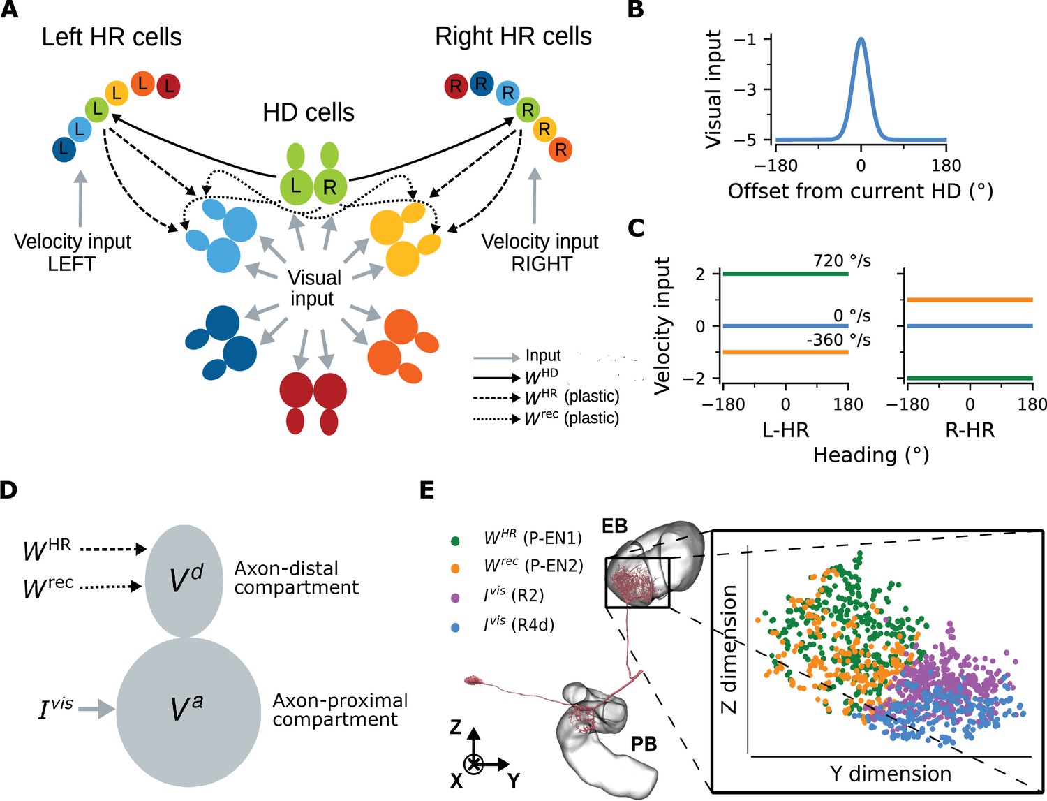
Network architecture.
(A) The ring of HD cells projects to two wings of HR cells, a leftward (Left HR cells, abbreviated as L-HR) and a rightward (Right HR cells, or R-HR), so that each wing receives selective connections only from a specific HD cell (L: left, R: right) for every head direction. For illustration purposes, the network is scaled-down by a factor of 5 compared to the cell numbers in the model. The schema shows the outgoing connections ( and ) only from the green HD neurons and the incoming connections ( and ) only to the light blue and yellow HD neurons. Furthermore, the visual input to HD cells and the velocity inputs to HR cells are indicated. (B) Visual input to the ring of HD cells as a function of radial distance from the current head direction (see Equation 5). (C) Angular-velocity input to the wings of HR cells for three angular velocities: 720 (green), 0 (blue), and -360 (orange) deg/s (see Equation 10). (D) The associative neuron: and denote the voltage in the axon-proximal (i.e. closer to the axon initial segment) and axon-distal (i.e. further away from the axon initial segment) compartment, respectively. Arrows indicate the inputs to the compartments, as in (A), and is the visual input current. (E) Left: skeleton plot of an example HD (E-PG) neuron (Neuron ID =416642425) created using neuPrint (Clements et al., 2020) the ellipsoid body (EB) and protocerebral bridge (PB) are overlayed. Right: zoomed in area in the EB indicated by the box, showing postsynaptic locations in the EB for this E-PG neuron; for details, see Methods. The neuron receives recurrent and HR input (green and orange dots, corresponding to inputs from P-EN1 and P-EN2 cells, respectively) and visual input (purple and blue dots, corresponding to inputs from visually responsive R2 and R4d cells, respectively) in distinct spatial locations.
Figure 1—figure supplement 1
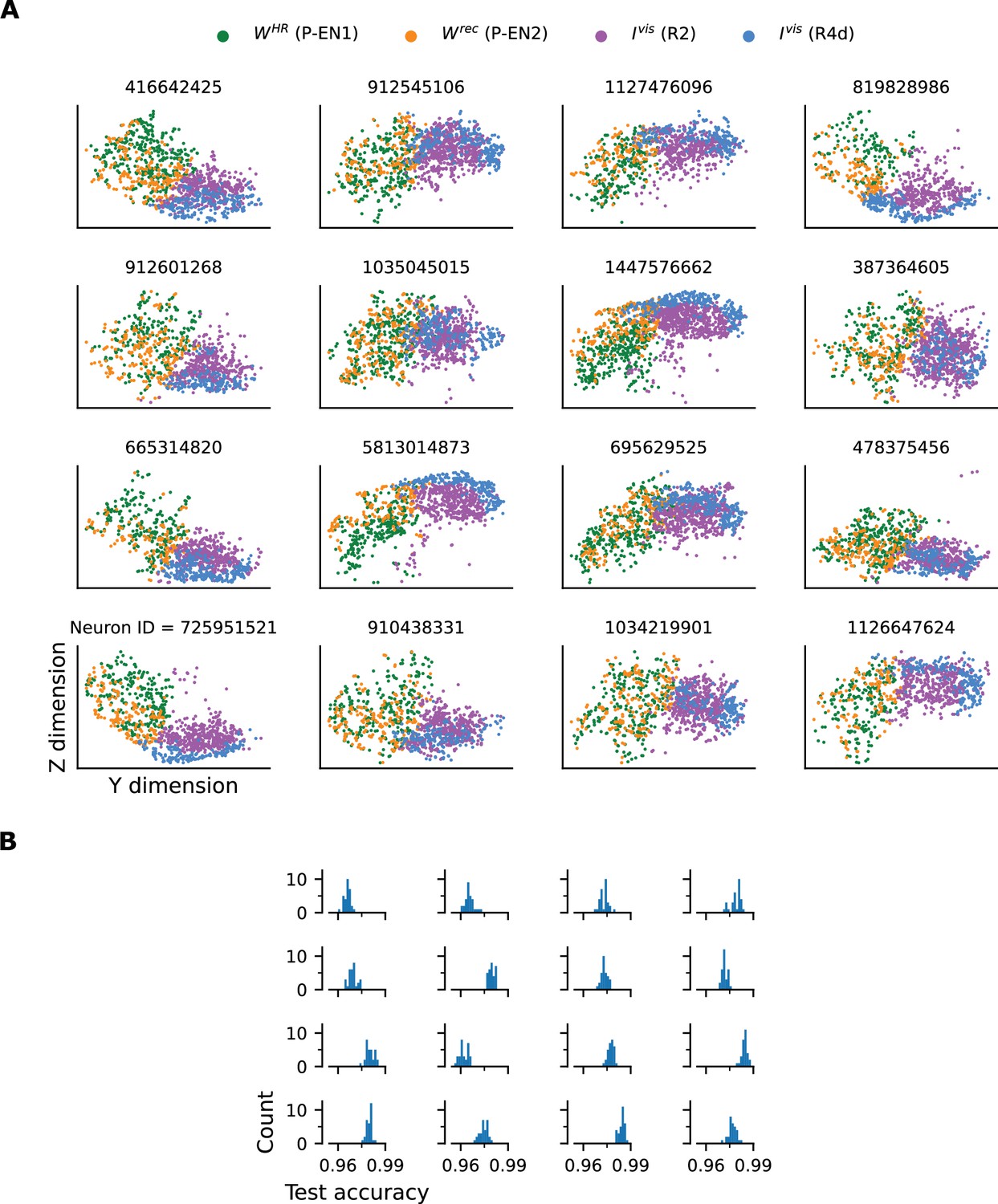
Separation of axon-proximal and axon-distal inputs to HD (E-PG) neurons in the Drosophila EB.
(A) Synaptic locations in the EB where visual (R2 and R4d) and recurrent and HR-to-HD (P-EN1 and P-EN2) inputs arrive, for a total of 16 HD neurons tested (Neuron ID above each panel). Similarly to the example in Figure 1E (repeated here in the top left panel, Neuron ID 416642425), these two sets of inputs appear to arrive in separate locations. (B) Binary classification between the two classes (R2 and R4d vs. P-EN1 and P-EN2) using SVMs with Gaussian kernel. Nested 5-fold crossvalidation was performed 30 times for every neuron tested, and the test accuracy histograms per neuron are plotted. The two classes can be separated with a test accuracy greater than 0.95 for every neuron.
Figure 1—video 1
A three-dimensional rotating video of the synapse locations in Figure 1E.
Figure 2
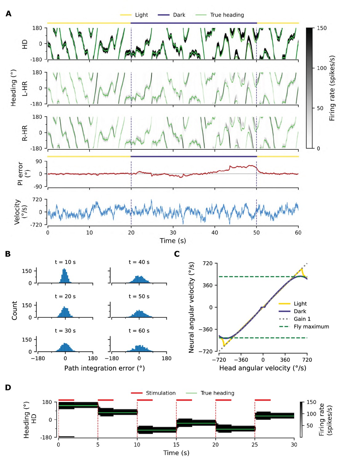
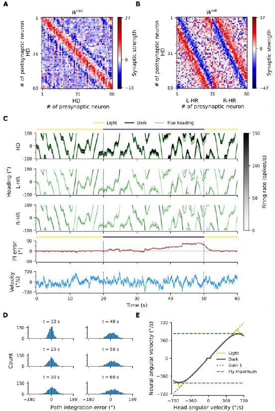
Path integration (PI) performance of the network.
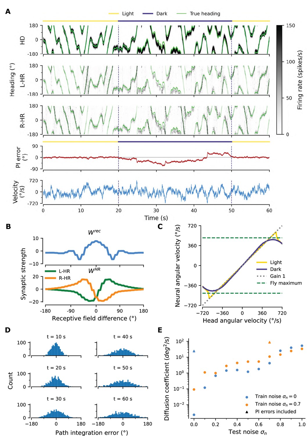
(A) Example activity profiles of HD, L-HR, and R-HR neurons (firing rates gray-scale coded). Activities are visually guided (yellow overbars) or are the result of PI in the absence of visual input (purple overbar). The ability of the circuit to follow the true heading is slightly degraded during PI in darkness. The PI error, that is, the difference between the PVA and the true heading of the animal as well as the instantaneous head angular velocity are plotted separately. (B) Temporal evolution of the distribution of PI errors in darkness, for 1000 simulations. The distribution gets wider with time, akin to a diffusion process. We estimate the diffusion coefficient to be (see ‘Diffusion Coefficient’ in Materials and methods). Note that, unless otherwise stated, for this type of plot we limit the range of angular velocities to those normally exhibited by the fly, i.e. deg/s. (C) Relation between head angular velocity and neural angular velocity, i.e., the speed with which the bump moves in the network. There is almost perfect (gain 1) PI in darkness for head angular velocities within the range of maximum angular velocities that are displayed by the fly (dashed green horizontal lines; see Methods). (D) Example of consecutive stimulations in randomly permeated HD locations, simulating optogenetic stimulation experiments in Kim et al., 2017. Red overbars indicate when the network is stimulated with stronger than normal visual-like input, at the location indicated by the animal’s true heading (light green line), while red dashed vertical lines indicate the onset of the stimulation. The network is then left in the dark. Our simulations show that the bump remains at the stimulated positions.
Figure 3 with 3 supplements
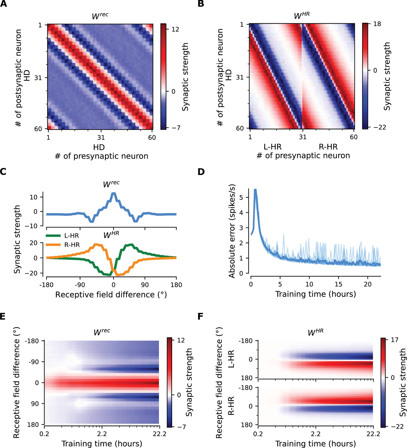
The network connectivity during and after learning.
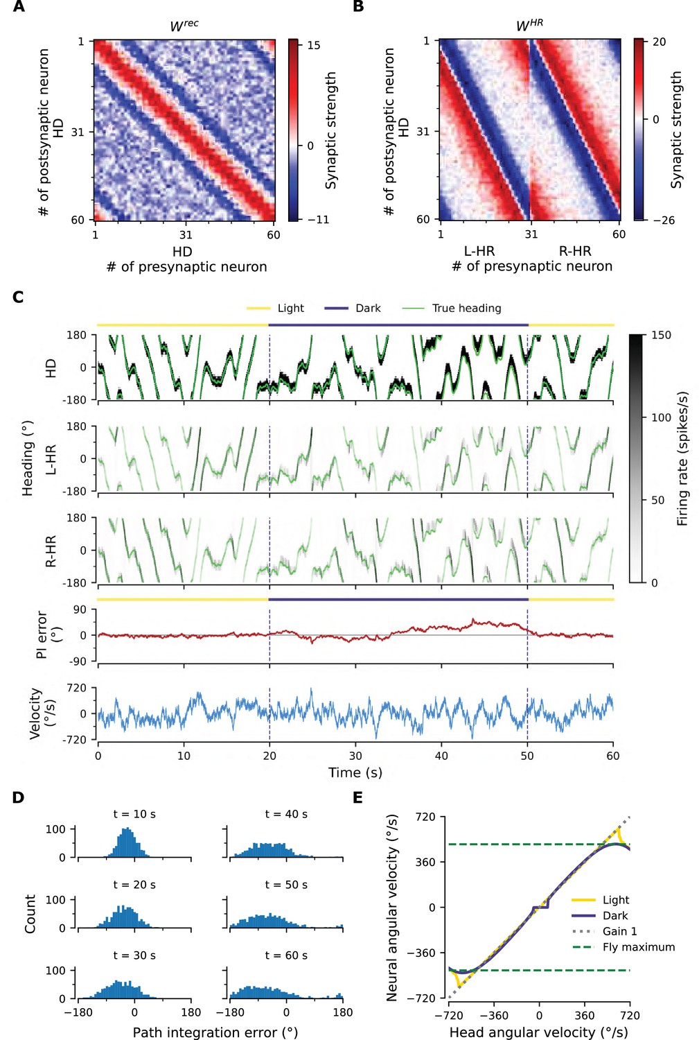
(A), (B) The learned weight matrices (color coded) of recurrent connections in the HD ring, , and of HR-to-HD connections, , respectively. Note the circular symmetry in both matrices. (C) Profiles of (A) and (B), averaged across presynaptic neurons. (D) Absolute learning error in the network (Equation 19) for 12 simulations (transparent lines) and average across simulations (opaque line). At time , we initialize all the plastic weights at random and train the network for s (∼22 hr). The mean learning error increases in the beginning while a bump in is emerging, which is necessary to generate a pronounced bump in the network activity. For weak activity bumps, absolute errors are small because the overall network activity is low. After ∼1 hr of training, the mean learning error decreases with increasing training time and converges to a small value. (E), (F) Time courses of development of the profiles of and , respectively. Note the logarithmic time scale.
Figure 3—figure supplement 1
Removal of long-range excitatory projections impairs PI for high angular velocities.
Figure 3—figure supplement 2
Details of learning.
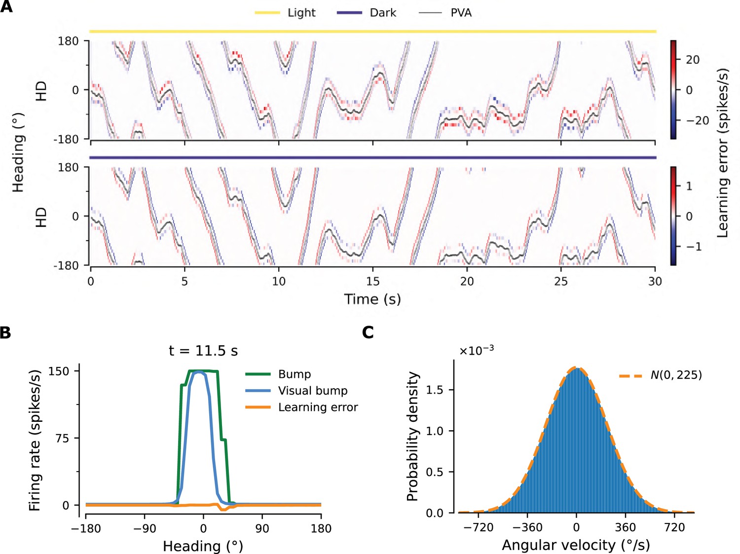
(A) Learning errors (Equation 18) in the converged network in light conditions (yellow overbar) or during PI in darkness (purple overbar). Note the difference in scale. In light conditions, the error is zero in all positions apart from the edges of the bump, where the error is substantial. Such errors occur because the velocity pathway, which implements PI, cannot move the bump for very small angular velocities, and tends to move it slightly faster for intermediate velocities, and slower for large ones (see Figure 2C). The velocity pathway is active and affects network activity even in the presence of visual input; hence, in light conditions, it creates errors at the edges of the bump, and the sign of the errors is consistent with the aforementioned PI velocity biases. Other than that, the angular velocity input predicts the visual input near-perfectly, as evidenced by the near-zero error everywhere else in the network. During PI in darkness, the network operates in a self-consistent manner, merely integrating the angular velocity input, and the learning error is much smaller. (B) Snapshot of the bump and the errors at s in light conditions from (A). Also overlaid is the hypothetical form of the bump if only the visual input was present in the axon-proximal compartment of the HD neurons, termed ‘Visual bump’. Notice that the errors are due to the fact that the visual bump is trailing in relation to the bump in the network. As a result, at the front of the bump the subthreshold visual input is actually inhibiting the bump. Also note that the bump in the network has a square form, in contrast to the smoother form that would be expected from visual input alone. This is because the learning rule in Equation 12 only converges when HD neurons reach saturation (see also panel A2). (C) Histogram of entrained velocities.
Figure 3—figure supplement 3
PI performance of a perturbed network.
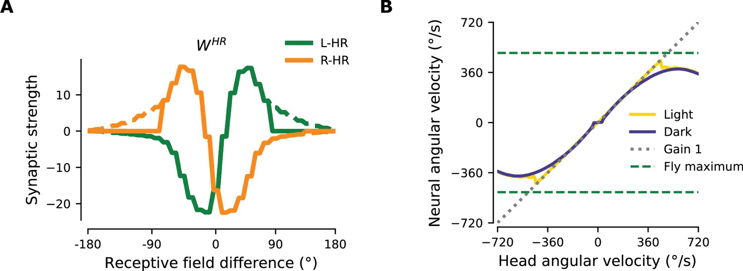
After learning, the synaptic connections in Figure 3A and B have been perturbed with Gaussian noise with standard deviation ∼1.5. (A), (B) Synaptic weight matrices after noise addition. (C) Example of PI. The activity of HD, L-HR, and R-HR neurons along with the PI error and instantaneous angular velocity are displayed, as in Figure 2A. (D) Temporal evolution of distribution of PI errors during PI in darkness. Compared to Figure 2B the distribution widens faster, and also exhibits side bias. (E) PI is impaired compared to Figure 2C, particularly for small angular velocities. Note that the exact form of the PI gain curve at very small angular velocities may vary slightly depending on the noise realization, but the findings mentioned in the Results (middle part of last paragraph of section ‘Learning results in synaptic connectivity that matches the one in the fly’) remain consistent.
Figure 4 with 1 supplement
The network adapts rapidly to new gains.
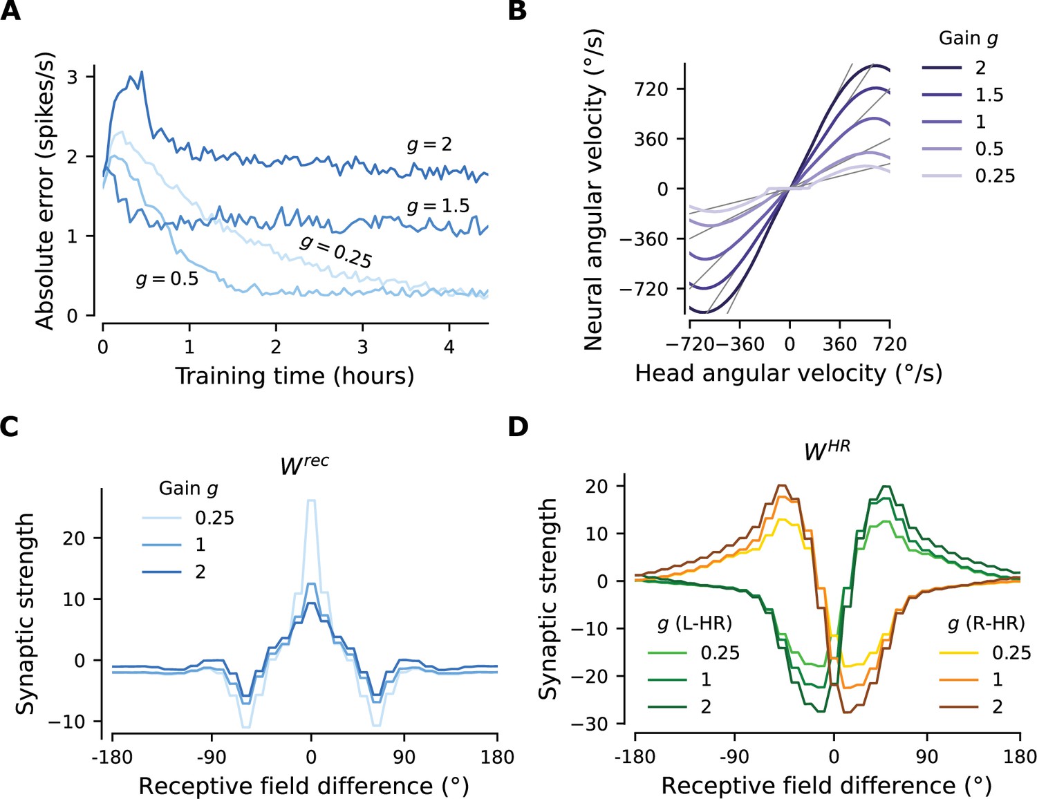
Starting from the converged network in Figure 3, we change the gain between visual and self-motion inputs, akin to experiments conducted in VR in flies and rodents (Seelig and Jayaraman, 2015; Jayakumar et al., 2019). (A) The mean learning error averaged across 12 simulations for each gain. After an initial increase due to the change of gain, the errors decrease rapidly and settle to a lower value. The steady-state values depend on the gain due to the by-design impairment of high angular velocities, which affects high gains preferentially. Crucially, adaptation to a new gain is much faster than learning the HD system from scratch (Figure 3D). (B) Velocity gain curves for different gains. The network has remapped to learn accurate PI with different gains for the entire dynamic range of head angular velocity inputs (approx. [-500, 500] deg/s). (C), (D) Final profiles of and , respectively, for different gains.
Figure 4—figure supplement 1
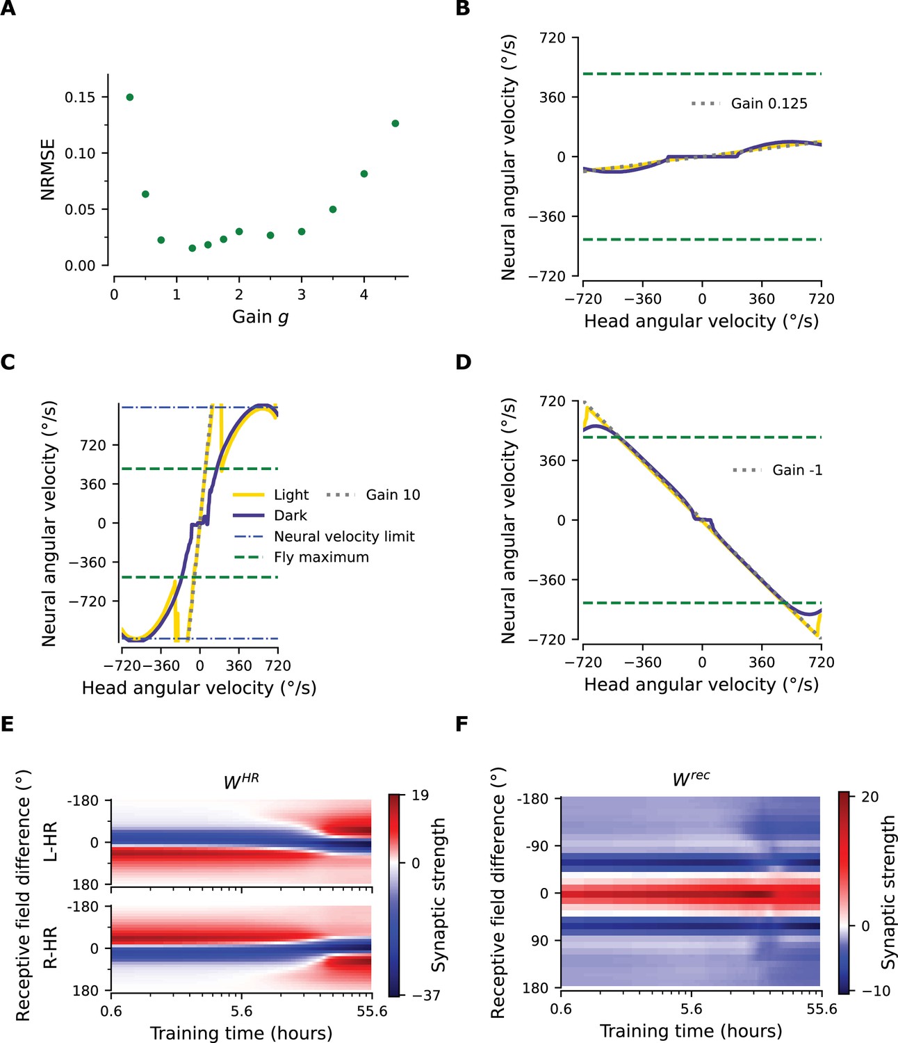
Limits of PI gain adaptation.
(A) Normalized root mean square error (NRMSE) between neural and head angular velocity, for gain-1 networks that subsequently have been rewired to learn different gains. To compute the NRMSE, we first estimate from PI performance plots (examples in (B), (C), and (D)) the root mean square error (RMSE) between the neural and head angular velocity, but only within the range of head angular velocities that each network can handle. This range is restricted because there is a maximum neural angular velocity (e.g. blue dot-dashed line in C; see also Appendix 1—figure 1A); thus the range of head angular velocity is given by this maximum neural angular velocity divided by the gain . Then, to obtain the NRMSE we divide the RMSE by that range. For instance, in (C), and deg/s. Then the head angular velocity range we test is determined by the x-coordinate for which the Gain-10 line (gray, dashed) meets the neural velocity limit line (blue, dot-dash); hence in this extreme example we only test for the range [-115, 115] deg/s. We find that rewiring performance is excellent for gains between 0.25 and 4.5, for which NRMSE is less than 0.15. Note that the more a new gain differs from original gain 1, the longer it takes for the network to rewire. (B), (C) PI performance plots for a small () and a large () gain. The NRMSE is 0.31 and 0.46, respectively. Performance is impaired because the flat area for small angular velocities gets enlarged in (B), whereas the network struggles to keep up with the desired gain in (C). (D) PI performance plot for a network that has been instructed to reverse its gain (from +1 to -1), i.e. when the visual and self-motion inputs are signaling movement in opposite directions. Performance is excellent, indicating that there is nothing special about negative gains; albeit learning takes considerably more time. (E), (F) Weight history for HR-to-HD and for recurrent connections, respectively, for the network trained to reverse its gain. The directionality of the asymmetric HR-to-HD connections in (E) reverses only after ∼20 hours, while the recurrent weights in (F) remain largely unaltered.
Appendix 1—figure 1
Robustness to injected noise.
(A) PI example in a network trained with noise (, train noise ). Panels are organized as in Figure 2A, which shows the activity in a network trained without noise (, ). (B) Profiles of learned weights. Both and are circularly symmetric. Panel is organized as in Figure 3C, which shows weight profiles in a network trained without noise (, ). (C) The network achieves almost perfect gain-1 PI, despite noisy inputs. Compared to Figure 2C the performance is only slightly impaired. (D) Temporal evolution of distribution of PI errors during PI in darkness. Compared to Figure 2B the distribution widens faster, however it also does not exhibit side bias. (E) Diffusion coefficient for networks as a function of the level of test noise (for details, see section "Diffusion Coefficient" in Materials and methods). We distinguish between networks that experienced noise during training (, orange) and networks that were trained without injected noise (, blue), which were studied in the Results of the main text. Diffusion coefficients that include contributions from PI errors, estimated from (D) and Figure 2B, are also plotted (triangles).
Appendix 2—figure 1

Limits of network performance when varying synaptic delays.
(A) Maximum neural angular velocity learned is inversely proportional to the synaptic delay in the network, with constant in Equation 23 (blue dot-dashed line). Green dots: point estimate of maximum neural velocity learned, green bars: 95% confidence intervals (Student’s t-test, ). (B) Example neural velocity gain plot (as in Figure 2C) in a network with increased synaptic delays ( increased from the "standard" value 65 ms to the new value 190 ms). (C) Behavior of the activity of HD cells in the network with parameters as in (B) near the velocity limit. The example network is driven by a single velocity in every column, in light (top row) and darkness (bottom row) conditions. In darkness, near and below the limit (left and middle column), there is a delay in the appearance of the bump, which then path-integrates with gain 1; above the limit observed in (B), however, the bump cannot stabilize, resulting in the dip in neural velocity (right column). (D) PI performance for a network with drastically reduced synaptic delays (). Compared to Figure 2C performance is worse for small angular velocities. This occurs because for small angular velocities, the offset of the HR bump in leftward vs. rightward movement is not as pronounced. As a result, it is harder to differentiate leftward from rightward movement. (E) For the same reason, the asymmetries in the learned HR-to-HD connectivity are not as prevalent as in Figure 3C.
Appendix 3—figure 1

Performance of a network where HD-to-HR connection weights are allowed to vary randomly, and HD neurons are projecting to HR neurons also adjacent to the ones they correspond to, respecting the topography of the protocerebral bridge (PB).
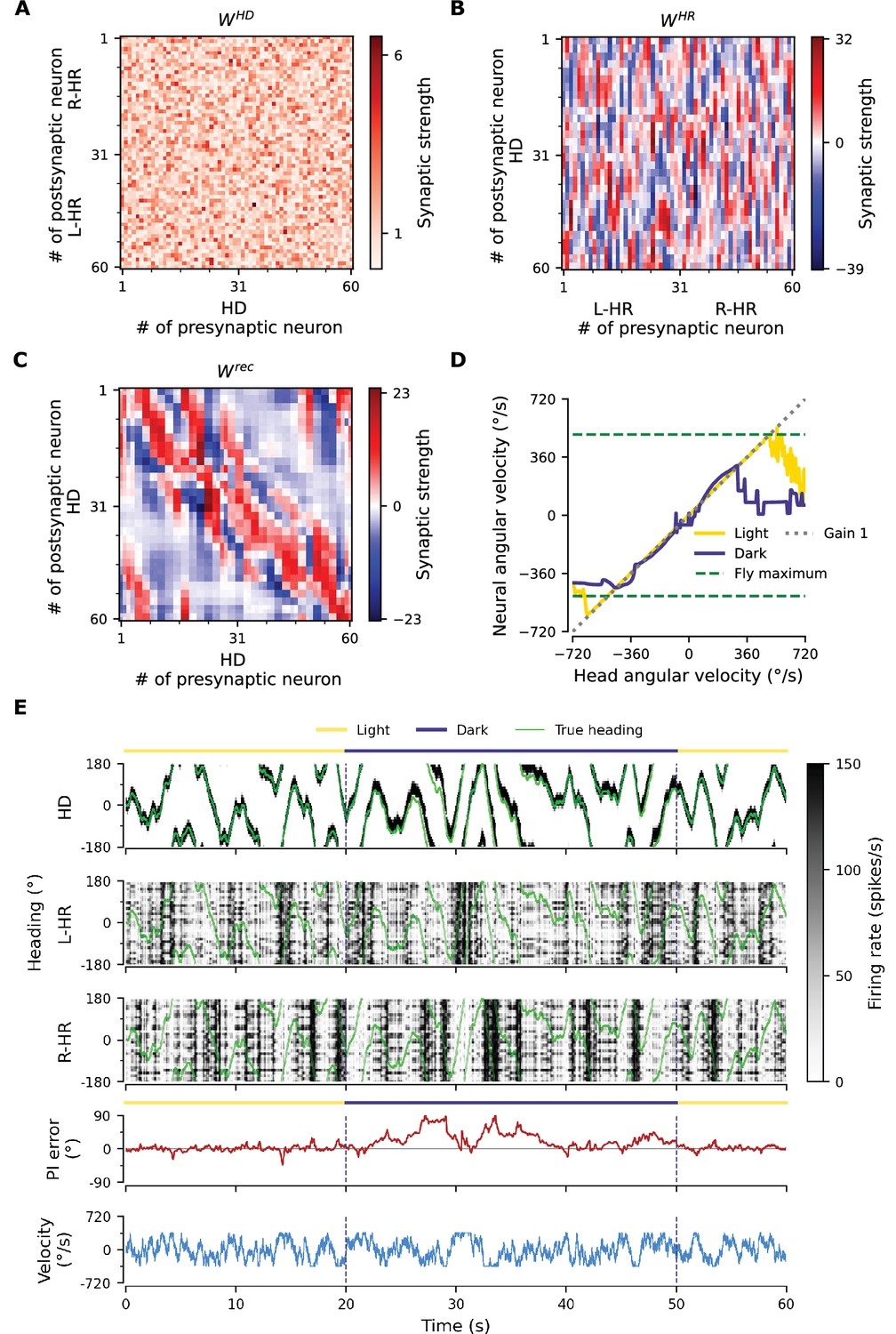
(A) The HD-to-HR connectivity matrix, . Note that, compared to what is described in the Materials and methods (final paragraph of ‘Neuronal Model’), the order of HD neurons is rearranged: we have grouped HD neurons that project to the same wing of the PB together, so that the diagonal structure of the connections is clearly visible. (B) The learned HR-to-HD connections, , depart from circular symmetry (as, e.g., in Figure 3B), so that asymmetries in could be counteracted. The recurrent connections (not shown) remain largely unaltered compared to the ones shown in Figure 3A. (C–E) Despite the randomization and lack of 1-to-1 nature of HD-to-HR connections, PI in the converged network remains excellent (Figure 2A–C).
Appendix 3—figure 2
PI performance in a network with random HD-to-HR connection strengths and learned weights from network in Figure 3.
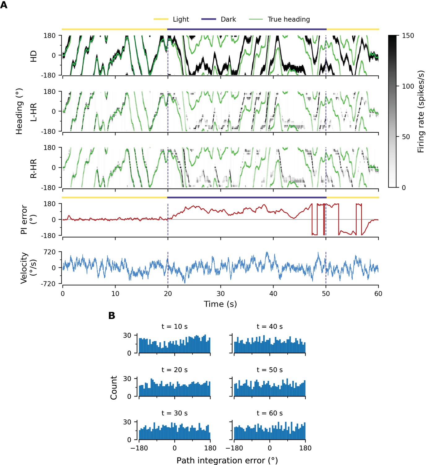
Here we vary the magnitude of the main diagonal HD-to-HR connections but preserve the 1-to-1 nature of the connections. We assume that and are passed down genetically (i.e. there is no further learning of these connections), and therefore the same, circular symmetric profiles apply to every location in the circuit. We choose these (assumed here to be genetically stored) profiles to be the ones we learned in the network outlined in Figure 3A and B. (A) Example that shows that PI is impaired, because the circular symmetric profiles passed down genetically cannot counteract small asymmetries in the architecture that are likely to be present in any biological system. Notice that it can even take several seconds for the large PI error to be corrected by the visual input. (B) PI errors grow fast (compare to e.g. Figure 2B). Already by of PI the heading estimate is random.
Appendix 3—figure 3
PI performance of a network where HD-to-HR connection weights are completely random.
(A) The HD-to-HR weights are drawn from a folded normal distribution, originating from a normal distribution with 0 mean and variance. (B) As a result, the learned HR-to-HD connections have also lost their structure. (C) The recurrent connections preserve some structure, since adjacency in the HD network is still important. (D) Impressively, the converged network can still PI with a gain close to 1, but for a reduced range of angular velocities compared to, e.g. the network in Appendix 3—figure 1. (E) A bump still appears in the HD network and gets integrated in darkness, albeit with larger errors. Note that bumps no longer appear in the HR populations; HR bumps are inherited from the HD bump only when adjacencies in the HD population are carried over to the HR populations by the HD-to-HR connections. Note that we have restricted angular velocities to the interval deg/s for this example, to showcase that PI is still accurate within this interval.
Appendix 5—figure 1
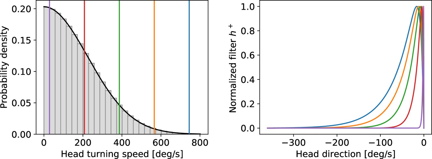
Left: assumed distribution of head-turning speeds (black) and discrete approximation used for the simulations.
The colored vertical lines indicate speeds for which the filter is plotted in the right panel. Right: temporal filter for several example speeds (see vertical lines in the left panel). Note that even for the largest speeds (blue curve) the filter decays within one turn around the circle.
Appendix 5—figure 2

Evolution of the reduced model.
The figure shows from top to bottom: (A) the HD-cells’ firing rate ; (B) the error ; (C) the average absolute error; (D) the recurrent weights ; (E–F) the rotation weights and . The HD firing rate and the errors (panels A-C) are averaged across speeds and both movement directions. The vertical dashed lines denote the time points shown in and Appendix 5—figure 4.
Appendix 5—figure 3
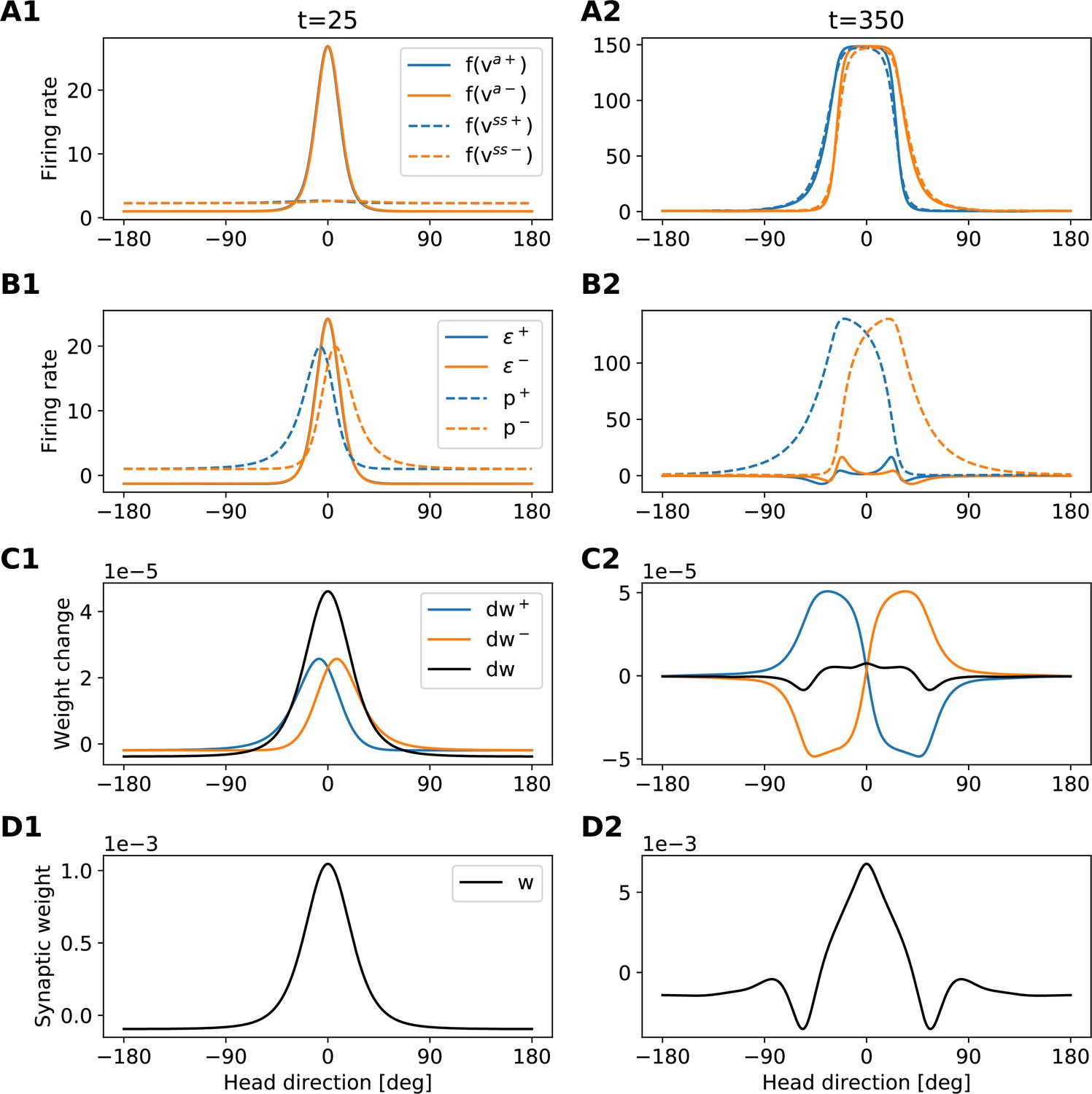
Development of the recurrent weights.
The figure provides an intuition for the shape of the recurrent-weights profiles that emerge during learning. Each column refers to a different time step (see also dashed lines in Appendix 5—figure 2). Each row shows a different set of variables of the model (see legends in the first column). The figure is to be read from top to bottom, because variables in the lower rows are computed from variables in the upper rows. Blue (orange) lines always refer to clockwise (anticlockwise) motion. Black lines in C show the total weight changes for both clockwise and anti-clockwise motion, that is, .
Appendix 5—figure 4
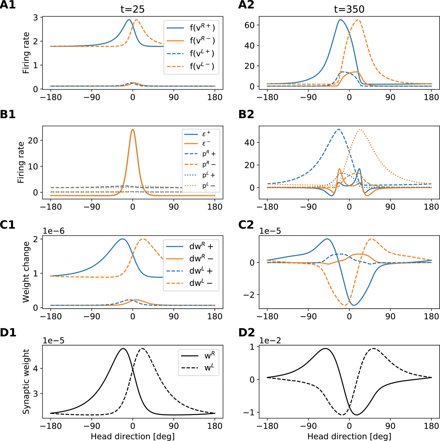
Development of the rotation weights.
The figure provides an intuition for the shape of the rotation-weights profiles that emerge during learning. Each column refers to a different time step (see also dashed lines in Appendix 5—figure 2). Each row shows a different set of variables of the model (see legends in the first column). The figure is to be read from top to bottom, because variables in the lower rows are computed from variables in the upper rows. Blue (orange) lines always refer to clockwise (anticlockwise) motion.
Author response image 1
PI performance of a network that was initialized with randomly shuffled weights from Fig.
3A,B. (A), (B) Resulting weight matrices after ~22 hours of training. The weights matrices look very similar to the ones in the main text in Fig. 3A,B, albeit connectivity remains noisy and weights span a larger range. (C) Example of PI shows that the network can still path-integrate accurately. (D) Temporal evolution of distribution of PI errors during PI in darkness. Performance is comparable to Fig. 2B of the main network, with only minimal side bias. (E) PI performance is comparable to the one in Fig. 2C.
Author response image 2

PI performance for networks with more neurons.
(A) For NHD = NHR = 120 and training time ~4.5 hours, PI performance is excellent, and the flat area for small angular velocities observed in Figure 2C is no longer present. (B) To confirm that small angular velocities are no longer impaired, we limit the range of tested velocities and reduce the interval between tested velocities to 0.5 deg/s. (C), (D) same as (A), (B), for NHD = NHR = 240 and training time ~2 hours.
Tables
Table 1
Parameter values.
| Parameter | Value | Unit | Explanation |
|---|---|---|---|
| 60 | Number of head direction (HD) neurons | ||
| 60 | Number of head rotation (HR) neurons | ||
| 12 | deg | Angular resolution of network | |
| 65 | ms | Synaptic time constant | |
| -1 | Global inhibition to HD neurons | ||
| 10 | ms | Leak time constant of axon-distal compartment of HD neurons | |
| 1 | ms | Capacitance of axon-proximal compartment of HD neurons | |
| 1 | Leak conductance of axon-proximal compartment of HD neurons | ||
| 2 | Conductance from axon-distal to axon-proximal compartment | ||
| 4 | Excitatory input to axon-proximal compartment in light conditions | ||
| 0 | Synaptic input noise level | ||
| 4 | Visual input amplitude | ||
| 16 | Optogenetic stimulation amplitude | ||
| 0.15 | Visual receptive field width | ||
| 0.25 | Optogenetic stimulation width | ||
| -5 | Visual input baseline | ||
| 150 | spikes/s | Maximum firing rate | |
| 2.5 | Steepness of activation function | ||
| 1 | Input level for 50% of the maximum firing rate | ||
| -1.5 | Global inhibition to HR neurons | ||
| 1/360 | s/deg | Constant ratio of velocity input and head angular velocity | |
| 2 | Input range for which has not saturated | ||
| ms | Constant weight from HD to HR neurons | ||
| 100 | ms | Plasticity time constant | |
| 0.5 | ms | Euler integration step size | |
| 0.5 | s | Time constant of velocity decay | |
| 450 | deg/ | Standard deviation of angular velocity noise | |
| 0.05 | 1 /s | Learning rate |
-
Parameter values, in the order they appear in the Methods section. These values apply to all simulations, unless otherwise stated. Note that voltages, currents, and conductances are assumed unitless in the text; therefore capacitances have the same units as time constants.
Appendix 4—table 1
Default values for time scales in the model ordered with respect to their magnitude.
| Time scale | Expression | Value | Unit |
|---|---|---|---|
| Membrane time constant of axon-proximal compartment | 1 | ms | |
| Membrane time constant of axon-distal compartment | 10 | ms | |
| Synaptic time constant | 65 | ms | |
| Weight update filtering time constant | 100 | ms | |
| Velocity decay time constant | 0.5 | s | |
| Learning time scale | 20 | s |
Additional files
Download links
A two-part list of links to download the article, or parts of the article, in various formats.
Downloads (link to download the article as PDF)
Open citations (links to open the citations from this article in various online reference manager services)
Cite this article (links to download the citations from this article in formats compatible with various reference manager tools)
Learning accurate path integration in ring attractor models of the head direction system
eLife 11:e69841.
https://doi.org/10.7554/eLife.69841


