Figures and data in Phase response analyses support a relaxation oscillator model of locomotor rhythm generation in Caenorhabditis elegans

Version of Record

Accepted for publication after peer review and revision.

Download
Cite
Share
CommentOpen annotations (there are currently 0 annotations on this page).

Version of Record published: November 1, 2021 (This version)
Accepted Manuscript published: September 27, 2021 (Go to version)
Accepted: September 24, 2021
Received: April 29, 2021
Preprint posted: June 23, 2020 (Go to version)

Figures
Videos
Tables
Additional files

8 figures, 1 video, 2 tables and 1 additional file

Figures

Figure 1

Download asset Open asset

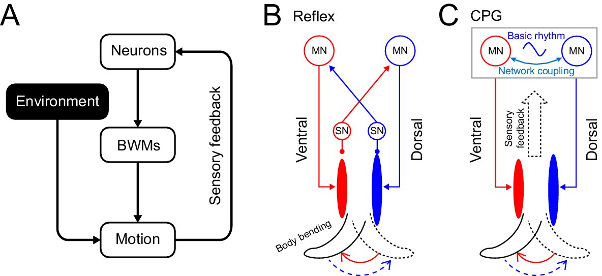
Rhythm generation in *C. elegans*.

(A) Motor neurons generate neuronal signals to control the activation of body wall muscles (BWM), which generates movement subject to internal and external environmental constraints. Sensory input provides feedback about body position and the environment. (**B,C**) Two possible models for locomotory rhythm generation in *C. elegans*. (B) In a reflex loop model, sensory neurons (SN) detect body postures and excite motor neurons (MN) to activate body wall muscles. (C) In a central pattern generator (CPG) model, network of motor neurons generates basic rhythmic patterns that are transmitted to body wall muscles while sensory feedback modulates the CPG rhythm. Diagrams (**B-C**) are adapted from Figure 1 in Marder and Bucher, 2001.

Figure 2 with 1 supplement

Download asset Open asset

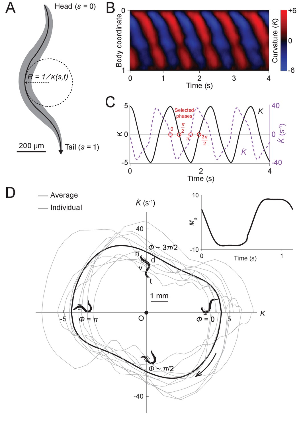
Undulatory dynamics of freely moving worms.

(A) Worm undulatory dynamics are quantified by the time-varying curvature along the body. The normalized body coordinate is defined by the fractional distance along the centerline (head = 0, tail = 1). The curvature $κ$ is the reciprocal of the local radius of curvature with positive and negative values representing dorsal and ventral curvature, respectively. (B) Curvature as a function of time and body coordinate during forward movement in a viscous liquid. Body bending curvature $K$ is represented using the nondimensional product of $κ$ and body length $L$ . (C) Curvature (black) in the anterior region (average over body coordinate 0.1-0.3) and the time derivative of curvature (dashed purple). Red circles mark four representative phases (0, $π / 2$ , $π$ , and $3 π / 2$ ). The curve is an average of 5041 locomotory cycles from 116 worms. (D) Phase portrait representation of the oscillatory dynamics of the anterior region, showing the curvature and the time derivative of the curvature parameterized by time. Images of worm correspond to the phases marked in (C). Arrow indicates clockwise movement over time. Dash-boxed region of the worm body indicates the 0.1–0.3 body coordinates. h: head; t: tail; v: ventral side; d: dorsal side. Gray curves are individual locomotory cycles from freely moving worms (10 randomly selected cycles are shown). (*Inset*) waveform of the scaled active muscle moment, estimated by equation $M_{a} = K + τ_{u} \dot{K}$ . Both curves were computed from the data used in (C).

Figure 2—figure supplement 1

Download asset Open asset

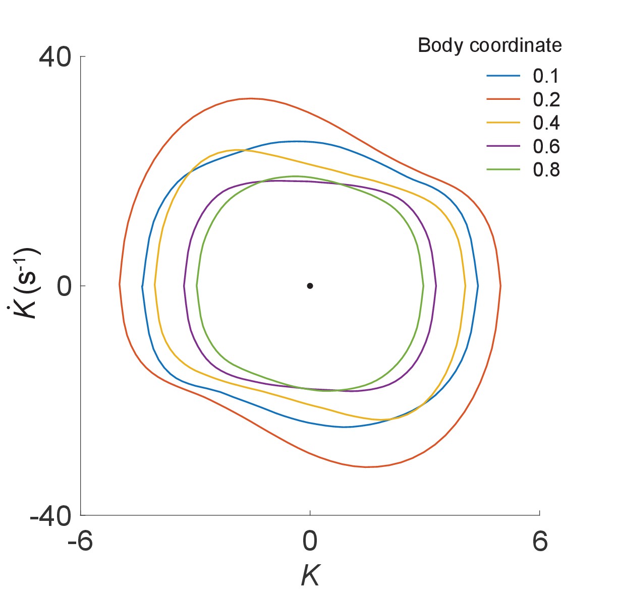
Phase portrait representations of the oscillatory bending dynamics for various body coordinates.

Figure 3 with 8 supplements

Download asset Open asset

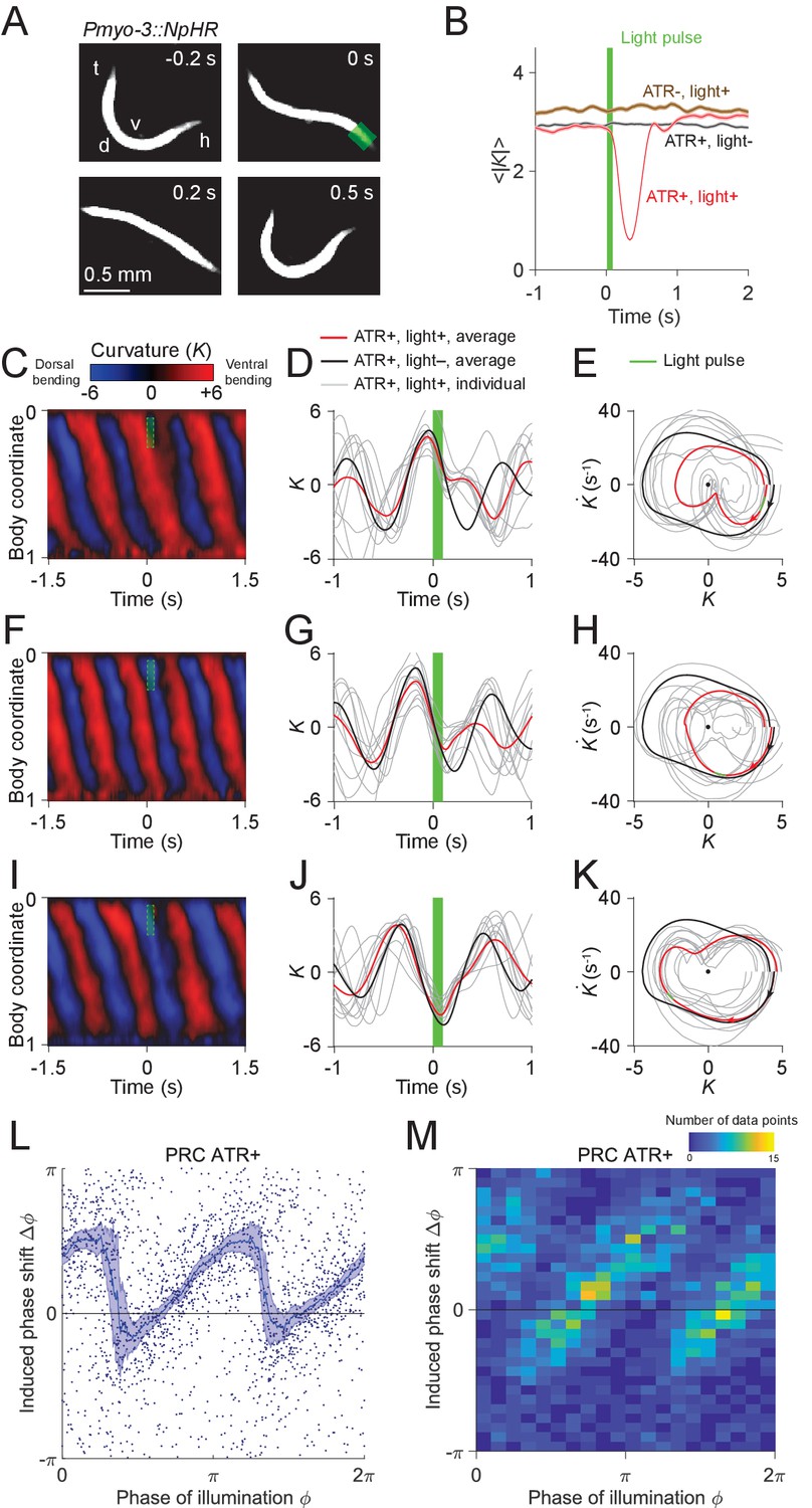
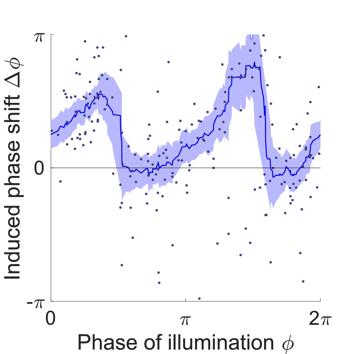
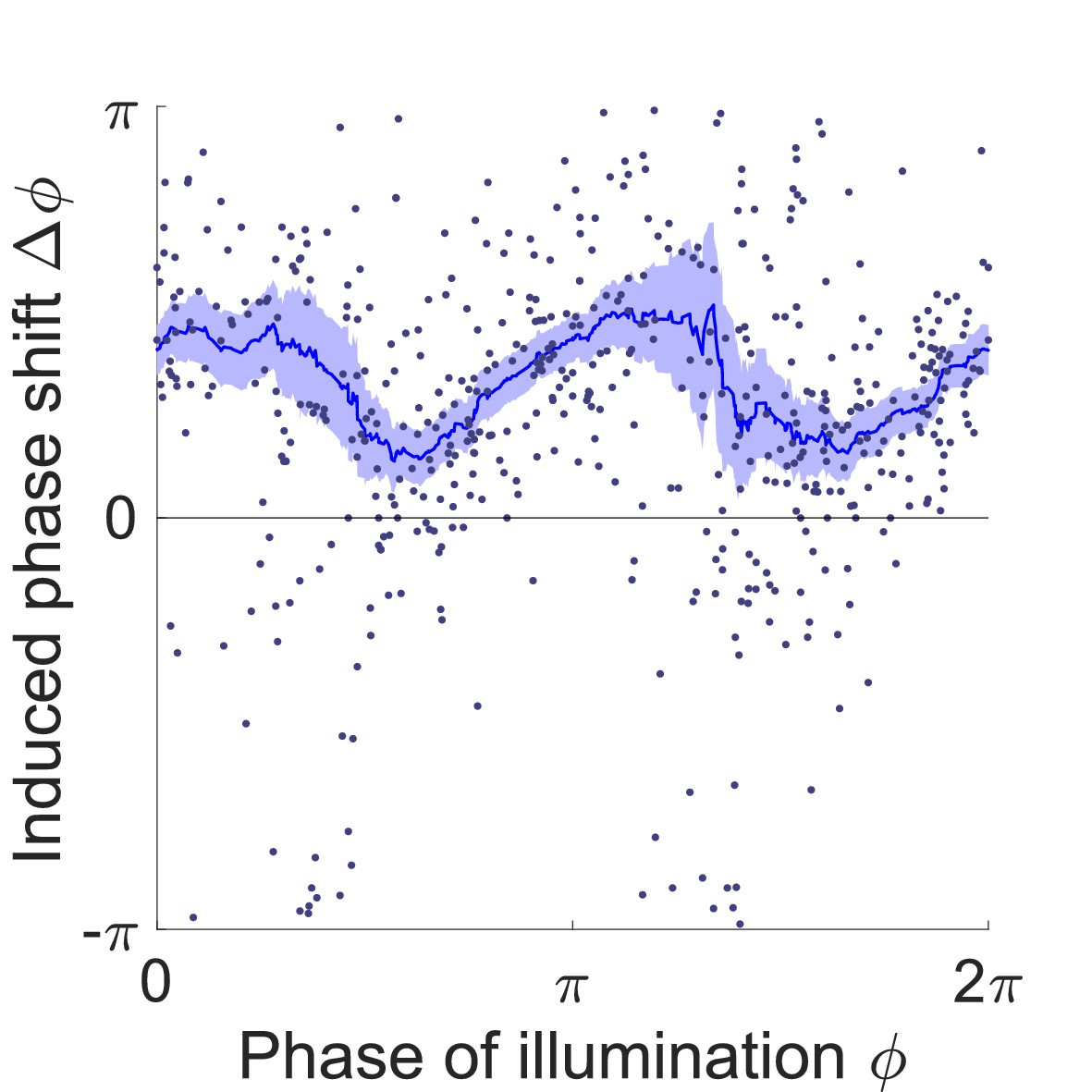
Analysis of phase-dependent inhibitions for head oscillation using transient optogenetic muscle inhibition.

(A) Images of a transgenic worm (*Pmyo-3::NpHR*) perturbed by a transient optogenetic muscle inhibition in the head during forward locomotion. Green shaded region indicates the 0.1 s laser illumination interval. h: head; t: tail; v: ventral side; d: dorsal side. (B) Effect of muscle inhibition on mean absolute curvature of the head. Black curve represents control ATR+ (no light) group (3523 measurements using 337 worms). Brown curve represents control ATR- group (2072 measurements using 116 worms). Red curve represents ATR+ group (1910 measurements using 337 worms). Green bar indicates 0.1 s light illumination interval starting at $t = 0$ . (**C-E**) Perturbed dynamics around light pulses occurring in the phase range $[0, π / 6]$ . (C) Kymogram of time-varying curvature $K$ around a 0.1 s inhibition (green dashed box). (D) Mean curvature dynamics around the inhibitions (green bar, aligned at $t = 0$ ) from ATR+ group (red curve, 11 trials using 4 worms) and control ATR+ (no light) group (black curve, eight trials using three worms). Gray curves are individual trials from ATR+ group (10 randomly selected trials are shown). (E) Mean phase portrait graphs around the inhibitions (green line) from ATR+ group (same trials as in D) and control group (ATR+, no light, 3998 trials using 337 worms). Gray curves are individual trials from ATR+ group. (**F-H**) Similar to (**C-E**), for phase range $[π / 3, π / 2]$ . (**I-K**) Similar to (**C-E**), for phase range $[2 π / 3, 5 π / 6]$ . (L) PRC from optogenetic inhibition experiments (ATR+ group, 991 trials using 337 worms, each point indicating a single illumination of one worm). The curve was obtained via a moving average along the x-axis with $0.16 π$ in bin width and the filled area represents 95% confidence interval within the bin. (M) A 2-dimensional histogram representation of the PRC using the same data. The histogram uses 25 bins for both dimensions, and the color indicates the number of data points within each rectangular bin.

Figure 3—figure supplement 1

Download asset Open asset

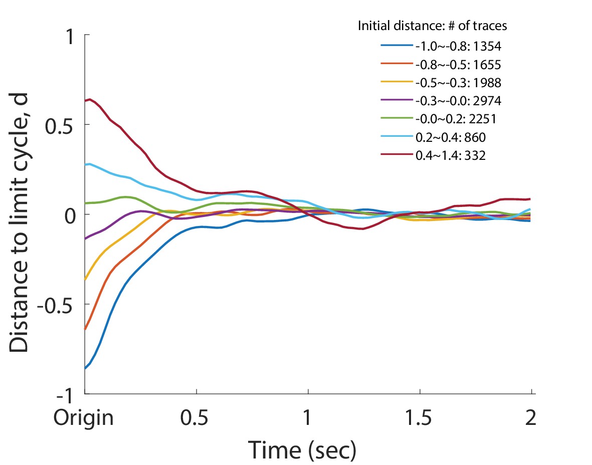
Normalized deviation to the normal cycle (the unperturbed oscillation) for the head oscillation of the perturbed worms.

Individual dynamics were grouped into different bins by binning their initial amplitude at $t = 0$ . In the figure, each trace represents the collective amplitude dynamics of the corresponding group. Distance $d$ is defined such that $d = - 1$ at the origin and $d = 0$ on the limit cycle. The legend indicates initial amplitude range of each bin and the corresponding number of individual traces within the bin.

Figure 3—figure supplement 2

Download asset Open asset

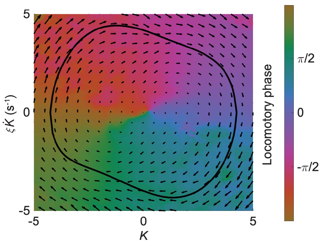
The isochron map overlaid with the vector field for the worm’s head oscillation.

On the isochron map, a point on the normal cycle (black trajectory) and all other points off the normal cycle that share the same color form a manifold representing states having an equal phase (indicated by the color bar). On the vector field, an arrow represents the phase state $(d K / d t, d (ξ \dot{K}) / d t)$ which determines the time derivative of the state of a trajectory. Both maps were computed from the results of experiments with *Pmyo-3::NpHR* worms.

Figure 3—figure supplement 3

Download asset Open asset

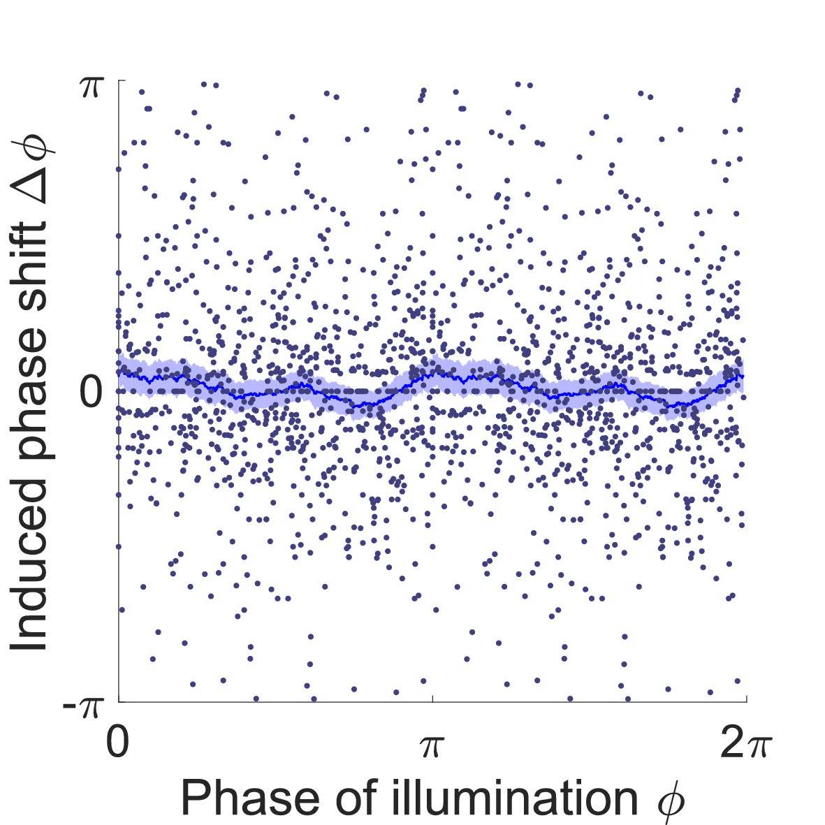
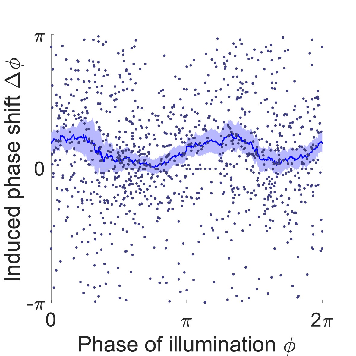
Phase response curve of *Pmyo-3::NpHR* worms (ATR- control group).

Curve was obtained from 414 trials of transient illuminations on head using 116 worms. Each point represents a single illumination (0.1 s duration, 532 nm wavelength) of one worm. Filled area represents 95% confidence interval.

Figure 3—figure supplement 4

Download asset Open asset

Phase response curve of *Pmyo-3::NpHR* worms perturbed by a 0.055 s optogenetic muscle inhibition during normal locomotion.

Curve was obtained from 150 trials of transient inhibitions of head muscles using 115 worms. Each point represents a single illumination (0.055 s duration, 532 nm wavelength) of one worm. Filled area represents 95% confidence interval.

Figure 3—figure supplement 5

Download asset Open asset

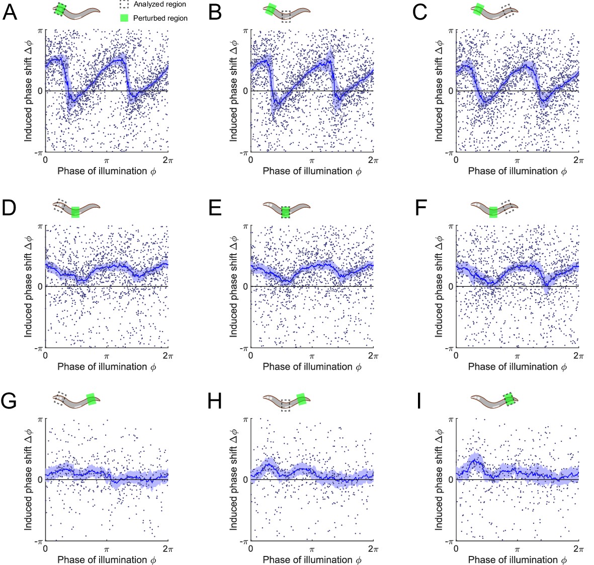
Phase response curves of *Pmyo-3::NpHR* worms induced by a 0.1 s optogenetic muscle inhibition, perturbed and measured at various body regions.

Anterior = 0.1-0.3; middle = 0.4-0.6; posterior = 0.6-0.8 along the worm body. (*Upper*) Schematics illustrating the selected spatial regions for optogenetic inhibition (Green shaded area) and phase response analysis (dashed box). (**A–C**) PRCs induced by muscle inhibition of the anterior region (991 trials using 337 worms), measured from (A) anterior, (B) middle, and (C) posterior regions, respectively. (**D–F**) PRCs induced by muscle inhibition of the middle region (687 trials using 276 worms), measured from (D) anterior, (E) middle, and (F) posterior regions, respectively. (**G–I**) PRCs induced by muscle inhibition of the posterior region (235 trials using 76 worms), measured from (G) anterior, (H) middle, and (I) posterior regions, respectively. For all the above plots, each point indicates a single illumination (0.1 s duration, 532 nm wavelength) of one worm. Experimental curves were obtained using a moving average along the x-axis with 0.16π in bin width. Filled area of each curve represents 95% confidence interval with respect to each bin of data points.

Figure 3—figure supplement 6

Download asset Open asset

Phase response curve of transgenic worms that express *NpHR* in all cholinergic neurons (*Punc-17::NpHR::ECFP*).

Curve was obtained from 270 trials of transient inhibitions of cholinergic neurons in the head region using 135 worms. Each point represents a single illumination (0.055 s duration, 532 nm wavelength) of one worm. Filled area represents 95% confidence interval.

Figure 3—figure supplement 7

Download asset Open asset

Phase response curve of transgenic worms that express Arch in the B-type motor neurons (*Pacr-5::Arch-mCherry*).

Curve was obtained from 551 trials of transient inhibitions of the B-type motor neurons in the head region using 160 worms. Each point represents a single illumination (0.055 s duration, 532 nm wavelength) of one worm. Filled area represents 95% confidence interval.

Figure 3—figure supplement 8

Download asset Open asset

Phase response curve of transgenic worms that express *NpHR* in the body wall muscles but lack the GABA receptor for the D-type motor neurons (*Pmyo-3::NpHR; unc-49(e407)*).

Curve was obtained from 259 trials of transient inhibitions of head muscles using 192 worms. Each point represents a single illumination (0.1 s duration, 532 nm wavelength) of one worm. Filled area represents 95% confidence interval.

Figure 4 with 1 supplement

Download asset Open asset

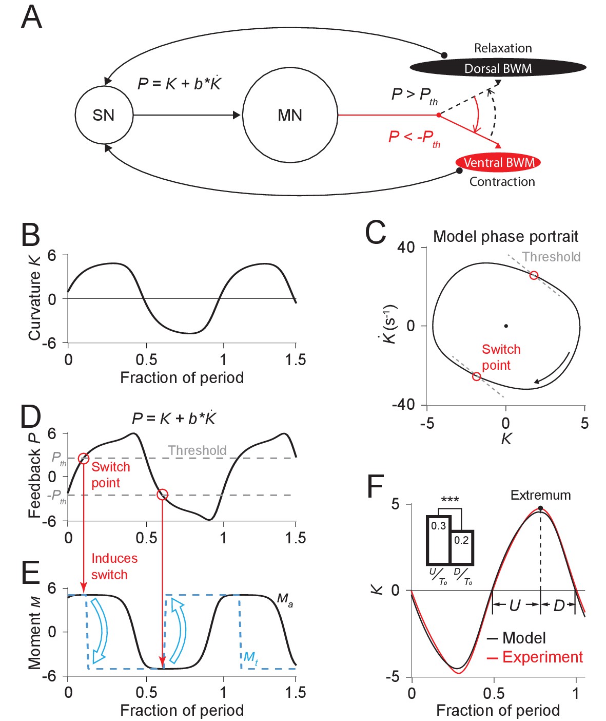
Free-running dynamics of a bidirectional relaxation oscillator model.

(A) Schematic diagram of the relaxation oscillator model. In this model, sensory neurons (SN) detect the total curvature of the body segment as well as the time derivative of the curvature. The linear combination of the two values, $P = K + b \dot{K}$ , is modeled as the proprioceptive signal which is transmitted to motor neurons (MN). The motor neurons alternatingly activate dorsal or ventral body wall muscles (BWM) based on a thresholding rule: (1) if $P < - P_{t h}$ , the ventral body wall muscles get activated and contract while the dorsal side of muscles relax; (2) if $P > P_{t h}$ , vice versa. Hence, locomotion rhythms are generated from this threshold-switch process. (B) Time-varying curvature $K$ of the model oscillator. The time axis is normalized with respect to oscillatory period (same for D, E, and F). (C) Phase portrait graph of the model oscillator. Proprioceptive threshold lines (gray dashed lines) intersect with the phase portrait graph at two switch points (red circles) at which the active moment of body wall muscles is switched. (D) Time-varying proprioceptive feedback $P$ received by the motor neurons. Horizontal lines denote the proprioceptive thresholds (gray dashed lines) that switch the active muscle moment at switch points (red circles, intersections between the proprioceptive feedback curve and the threshold lines). (E) Time-varying active muscle moment. Blue-dashed square wave denotes target moment ( $M_{t}$ ) that instantly switches directions at switch points. Black curve denotes the active muscle moment ( $M_{a}$ ) which follows the target moment in a delayed manner. (F) Time varying curvature in the worm’s head region from experiments (red, 5047 cycles using 116 worms) and model (black). Model curvature matches experimental curvature with an MSE ≈ 0.18. (*Inset*) Bar graph of $U$ (time period of bending toward the ventral or dorsal directions) and $D$ (time period of straightening toward a straight posture). Vertical bars are averages of fractions with respect to undulatory period $T_{0}$ of $U$ and $T$ (*** indicates p<0.0005 using Student’s t test).

Figure 4—figure supplement 1

Download asset Open asset

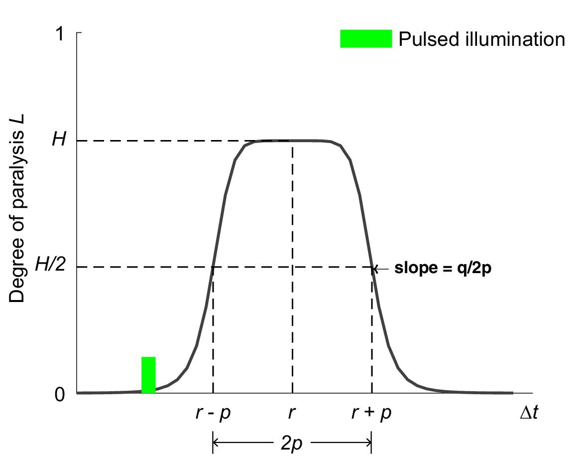
Bell-shaped function for modeling the optogenetic muscle inhibition (Equation A14).

The curve models the degree of paralysis due to the optogenetic muscle inhibition as a function of time. Referring to Equation A14, the fractional variable $H$ describes the reduced proportion of muscle moment when a worm reaches maximal paralysis after illumination. $r$ describes the time of maximal paralysis with respect to the occurrence of illumination. $p$ determines the time interval during which the paralyzing degree exceeds $H / 2$ . $q$ and $p$ together determine the paralyzing rate.

Figure 5 with 1 supplement

Download asset Open asset

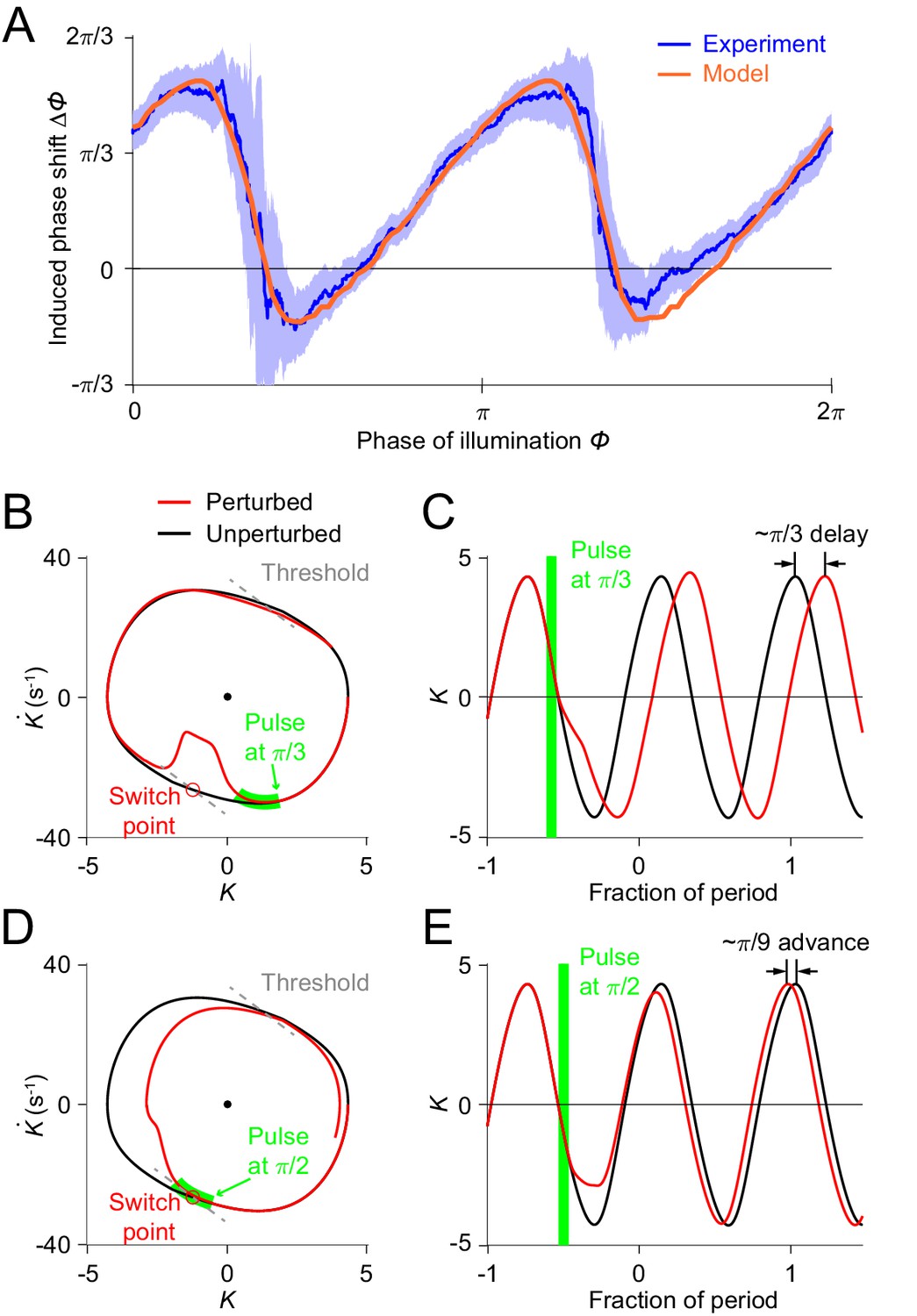
Simulations of optogenetic inhibitions in the relaxation oscillator model.

(A) Phase response curves measured from experiments (blue, same as in Figure 3L) and model (orange). Model PRC matches experimental PRC with an MSE ≈ 0.12. (**B,C**) Simulated dynamics of locomotion showing inhibition-induced phase delays in the model oscillator. (B) Simulated phase portrait graphs around inhibition occurring at $π / 6$ phase of cycle for perturbed (red) and unperturbed (black) dynamics. Green bar indicates the phase during which the inhibition occurs. (C) Same dynamics as in (B), represented by time-varying curvatures. The time axis is normalized with respect to oscillatory period (same for E). (**D,E**) Simulated dynamics of locomotion showing inhibition-induced phase advances in the model oscillator. (D) Simulated phase portrait graphs around inhibition occurring at $π / 2$ phase of cycle for perturbed (red) and unperturbed (black) dynamics. (E) Same dynamics as in (D), represented by time-varying curvatures.

Figure 5—figure supplement 1

Download asset Open asset

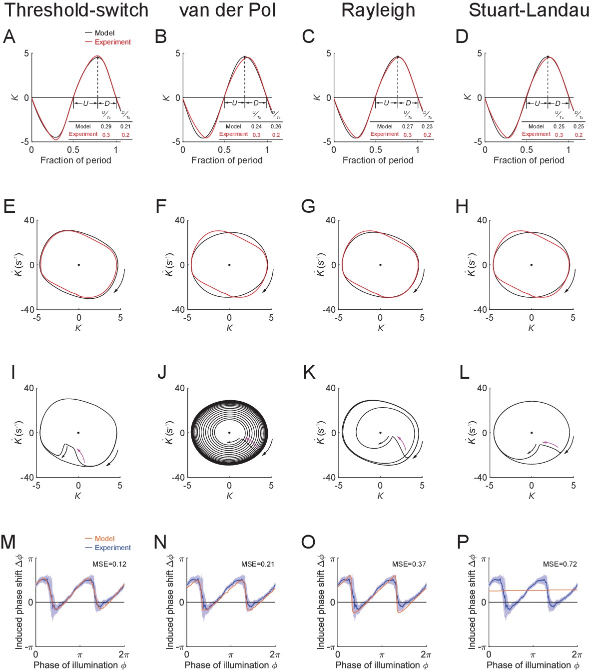
Performance of model oscillators: threshold-switch (column 1), van der Pol (column 2), Rayleigh (column 3), and Stuart-Landau (column 4).

(**A-D**) Time-varying curvatures of the worm’s head region, measured from experiments (red, 5047 cycles using 116 worms) or produced by models (black). The four models match the experimental curvature with MSEs ≈ 0.18, 0.44, 0.18, and 0.39, respectively. (Inset table) $U / T_{0}$ (fraction of period of bending toward the ventral or dorsal directions) and $D / T_{0}$ (fraction of period of straightening toward a straight posture), for experiments or models, respectively. (**E-H**) Phase portrait graphs of the free-running dynamics shown in (**A-D**), measured from experiments (red) or produced by models (black). Arrow indicates clockwise movement. (**I-L**) Phase plots showing each model perturbed (indicated by purple arrow) away from the stable limit cycle and then recovering toward the equilibrium. (**M-P**) Phase response curves with respect to both-side muscle inhibition, measured from experiments (blue, 991 trials using 337 worms) or produced by models (orange). Four models match the experimental PRC with MSE ≈ 0.12, 0.21, 0.37, and 0.72, respectively.

Figure 6 with 2 supplements

Download asset Open asset

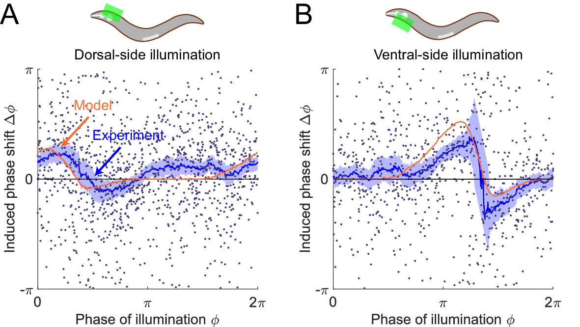
The model predicts phase response curves with respect to single-side muscle inhibitions.

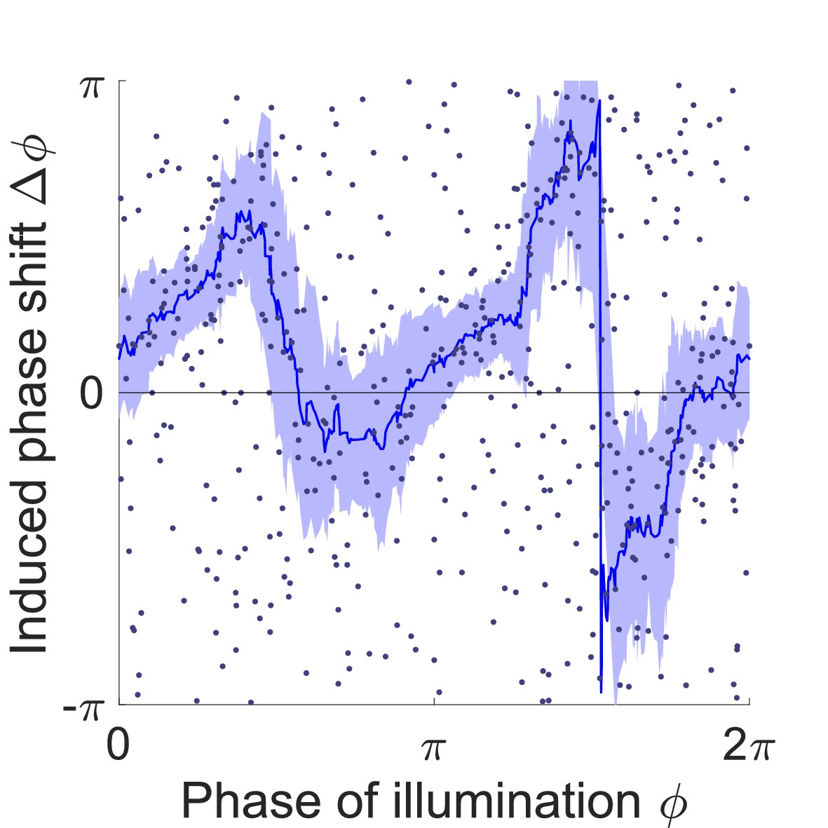
(A) (*Upper*) a schematic indicating a transient inhibition of body wall muscles of the head on the dorsal side. (*Lower*) the corresponding PRC measured from experiments (blue, 576 trials using 242 worms) and model (orange). (B) (*Upper*) a schematic indicating a transient inhibition of body wall muscles of the head on the ventral side. (*Lower*) the corresponding PRC measured from experiments (blue, 373 trials using 176 worms) and model (orange). For the two experiments, each point indicates a single illumination (0.1 s duration, 532 nm wavelength) of one worm. Experimental curves were obtained using a moving average along the x-axis with $0.16 π$ in bin width. Filled area of each experimental curve represents 95% confidence interval with respect to each bin of data points.

Figure 6—figure supplement 1

Download asset Open asset

Paralyzing effect analysis of muscle inhibitions induced by illumination on different sides of the worm’s head segment.

(A) Spectra of paralyzing effects across all phases of illuminations, represented by absolute curvature $| K |$ of the head region. $| K |$ shown on y-axis is the value obtained $0.53 π$ later in phase (or 0.3 s in time with respect to locomotion period 1.13 s) after the illumination phase $ϕ$ . The specific phase difference $0.53 π$ (or 0.3 s time difference) was chosen for computing the paralyzing effects because a max paralysis is achieved at ~0.3 s after illumination as shown in Figure 3B. Gray curve represents control ATR+ (no light) group (414 trials using 116 worms). Red curve represents ATR+ group with only ventral side being illuminated (373 trials using 176 worms). Blue curve represents ATR+ group with only dorsal side being illuminated (576 trials using 242 worms). Black curve represents ATR+ group with both sides being illuminated (991 trials using 337 worms). All curves were obtained using a moving average along the x-axis with $0.4 π$ in bin width and filled areas represent 95% confidence interval. (B) Average paralyzing effects during dorsal bend and ventral bend, represented by mean absolute curvature $⟨|K|⟩$ averaged across range $[0, π]$ (dorsal bend) and $[π, 2 π]$ (ventral bend), respectively. Colors indicate different conditions of experiment in the same way as in (A). (***) indicates p<0.0005 using paired t test.

Figure 6—figure supplement 2

Download asset Open asset

Phase response curves with respect to single-side muscle inhibition, simulated from model oscillators: threshold-switch (column 1), van der Pol (column 2), Rayleigh (column 3), and Stuart-Landau (column 4).

(**A-D**) PRCs with respect to dorsal-side muscle inhibition, measured from experiments (blue, 576 trials using 242 worms) or produced by models (orange). (**E-H**) PRCs with respect to ventral-side muscle inhibition, measured from experiments (blue, 373 trials using 176 worms) or produced by models (orange). Filled areas of all experimental PRCs represent 95% confidence interval with respect to each bin of data points.

Figure 7

Download asset Open asset

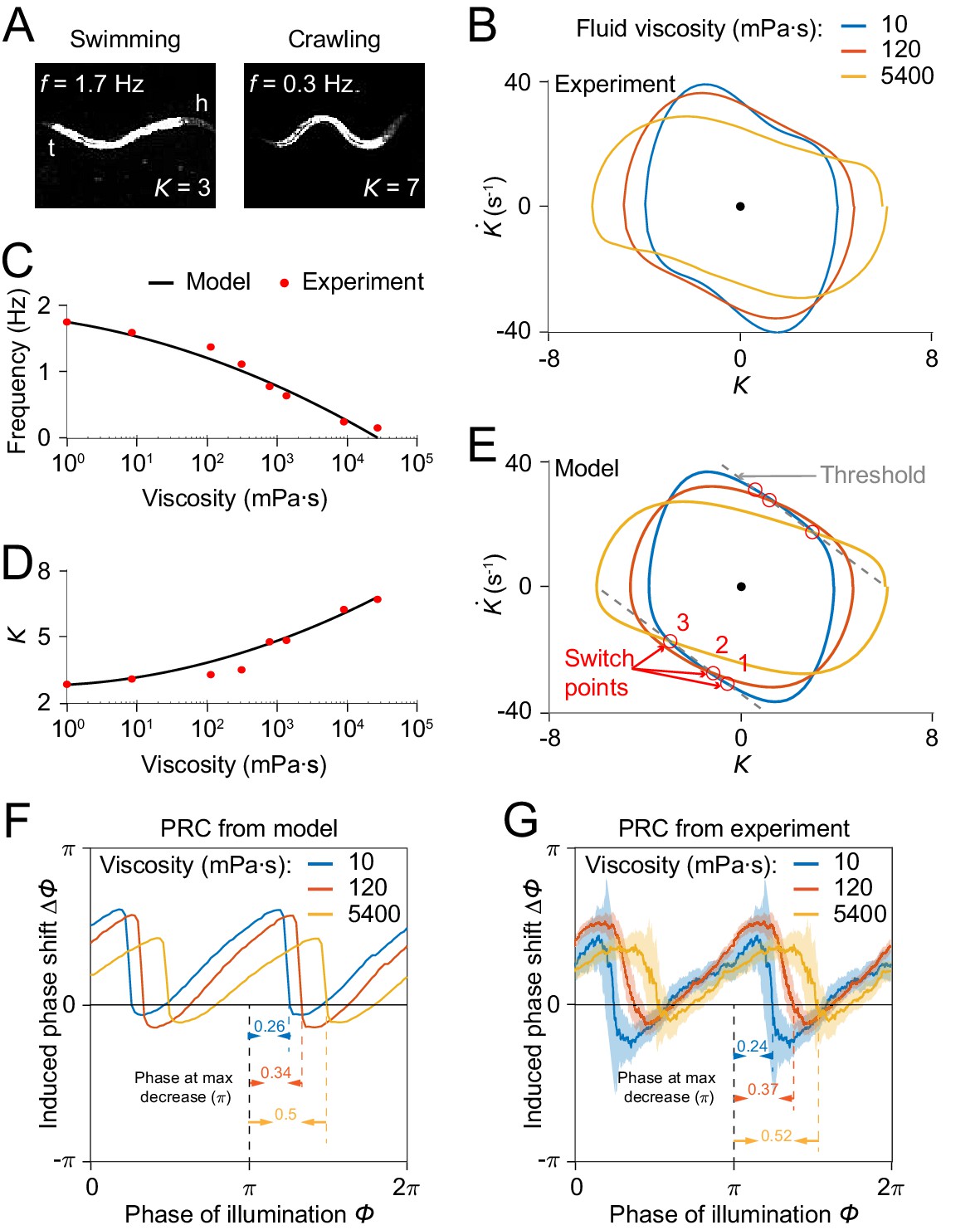
Model reproduces *C.elegans* gait adaptation to external viscosity.

(A) Dark field images and the corresponding undulatory frequencies and amplitudes of adult worms (*left*) swimming in NGM buffer of viscosity 1 mPa·s, (*right*) crawling on agar gel surface. The worm head is to the right in both images. (B) Phase portrait graphs measured from worm forward movements in fluids of viscosity 10 mPa·s (blue, 3528 cycles using 50 worms), 120 mPa·s (red, 5050 cycles using 116 worms), and 5400 mPa·s (yellow, 1364 cycles using 70 worms). (**C,D**) The model predicts the dependence of undulatory frequency (C) and curvature amplitude (D) on external viscosity (black) that closely fit the corresponding experimental observations (red). (E) Phase portrait graphs predicted from the model in three different viscosities (same values as in B). Gray dashed lines indicate threshold lines for dorsoventral bending. The intersections (red circles 1, 2, 3) between the threshold line and phase portrait graphs are switch points for undulations in low, medium, high viscosity, respectively. (F) Theoretically predicted PRCs in fluids of the three different viscosities show that PRC will be shifted to the right as the viscosity of environment increases. (G) PRCs measured from optogenetic inhibition experiments in the three viscosities. Experimental PRCs were obtained using a moving average along the x-axis with $0.16 π$ in bin width and filled areas are 95% confidence interval. The tendency of shift observed in experimental PRCs verified the model prediction.

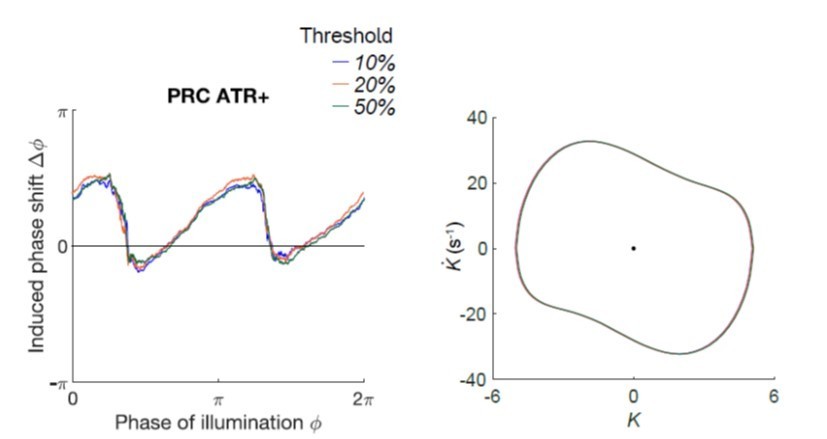
Author response image 1

Download asset Open asset

Videos

Video 1

Download asset

posterframe for video — Transient illumination of the anterior region of a freely moving *Pmyo-3::NpHR* worm.

Green-shaded region indicates timing and location of illumination.

Tables

Key resources table

Reagent type (species) or resource	Designation	Source or reference	Identifiers	Additional information
Strain, strain background (E. coli)	OP50	CGC	Fang-Yen Lab Strain Collection: OP50 RRID:WB-STRAIN:WBStrain00041971	OP50
Strain, strain background (C. elegans)	YX148	Fouad et al., 2018	Fang-Yen Lab Strain Collection: YX148	qhIs1[Pmyo-3::NpHR::eCFP; lin-15(+)]; qhIs4[Pacr-2::wCherry]
Strain, strain background (C. elegans)	YX119	Fouad et al., 2018	Fang-Yen Lab Strain Collection: YX119	qhIs1[Pmyo-3::NpHR::eCFP; lin-15(+)]; unc-49(e407)
Strain, strain background (C. elegans)	YX205	Leifer et al., 2011	Fang-Yen Lab Strain Collection: YX205	hpIs178[Punc-17::NpHR::eCFP; lin-15(+)]
Strain, strain background (C. elegans)	WEN001	Fouad et al., 2018	Fang-Yen Lab Strain Collection: WEN001	wenIs001[Pacr-5::Arch::mCherry; lin-15(+)]

Appendix 1—table 1

Objective functions used in the optimization procedures for alternative models.

Type	Free locomotion model	Complete model
van der Pol	$\underset{a_{V}, b_{V}, ω_{V}}{a r g m i n} ({(\frac{T_{v d P}}{T_{e x p t}} - 1)}^{2} + {(\frac{A_{v d P}}{A_{e x p}} - 1)}^{2})$	$\underset{p_{V}, H, q}{a r g m i n} \sum_{0}^{2 π} (P R C_{v d p} (ϕ) - P R C_{e x p} (ϕ))^{2} Δ ϕ$
Rayleigh	$\underset{a_{R}, b_{R}, ω_{R}}{a r g m i n} ({(\frac{T_{R a y l e i g h}}{T_{e x p t}} - 1)}^{2} + {(\frac{A_{R a y l e i g h}}{A_{e x p}} - 1)}^{2})$	$\underset{p_{R}, H, q}{a r g m i n} \sum_{0}^{2 π} (P R C_{R a y l e i g h} (ϕ) - P R C_{e x p} (ϕ))^{2} Δ ϕ$
Stuart-Landau	$\underset{a_{S}, b_{S}, ω_{S}}{a r g m i n} ({(\frac{T_{S L}}{T_{e x p t}} - 1)}^{2} + {(\frac{A_{S L}}{A_{e x p}} - 1)}^{2})$	$\underset{p_{S}, H, q}{a r g m i n} \sum_{0}^{2 π} (P R C_{S L} (ϕ) - P R C_{e x p} (ϕ))^{2} Δ ϕ$

Two-step optimization procedure for van der Pol, Rayleigh, and Stuart-Landau oscillators. The first-step optimization determines part of parameters such that individual models generate free locomotion dynamics. The second-step optimization leads to complete models such that models’ perturbed dynamics and phase response curves are produced.

Additional files

Transparent reporting form: https://cdn.elifesciences.org/articles/69905/elife-69905-transrepform-v2.docx
Download elife-69905-transrepform-v2.docx

Download links

A two-part list of links to download the article, or parts of the article, in various formats.

Downloads (link to download the article as PDF)

Open citations (links to open the citations from this article in various online reference manager services)

Mendeley

Cite this article (links to download the citations from this article in formats compatible with various reference manager tools)

Hongfei Ji
Anthony D Fouad
Shelly Teng
Alice Liu
Pilar Alvarez-Illera
Bowen Yao
Zihao Li
Christopher Fang-Yen

(2021)

Phase response analyses support a relaxation oscillator model of locomotor rhythm generation in Caenorhabditis elegans

eLife 10:e69905.

https://doi.org/10.7554/eLife.69905

Figures

Rhythm generation in C. elegans.

Undulatory dynamics of freely moving worms.

Phase portrait representations of the oscillatory bending dynamics for various body coordinates.

Analysis of phase-dependent inhibitions for head oscillation using transient optogenetic muscle inhibition.

Normalized deviation to the normal cycle (the unperturbed oscillation) for the head oscillation of the perturbed worms.

The isochron map overlaid with the vector field for the worm’s head oscillation.

Phase response curve of Pmyo-3::NpHR worms (ATR- control group).

Phase response curve of Pmyo-3::NpHR worms perturbed by a 0.055 s optogenetic muscle inhibition during normal locomotion.

Phase response curves of Pmyo-3::NpHR worms induced by a 0.1 s optogenetic muscle inhibition, perturbed and measured at various body regions.

Phase response curve of transgenic worms that express NpHR in all cholinergic neurons (Punc-17::NpHR::ECFP).

Phase response curve of transgenic worms that express Arch in the B-type motor neurons (Pacr-5::Arch-mCherry).

Phase response curve of transgenic worms that express NpHR in the body wall muscles but lack the GABA receptor for the D-type motor neurons (Pmyo-3::NpHR; unc-49(e407)).

Free-running dynamics of a bidirectional relaxation oscillator model.

Bell-shaped function for modeling the optogenetic muscle inhibition (Equation A14).

Simulations of optogenetic inhibitions in the relaxation oscillator model.

Performance of model oscillators: threshold-switch (column 1), van der Pol (column 2), Rayleigh (column 3), and Stuart-Landau (column 4).

The model predicts phase response curves with respect to single-side muscle inhibitions.

Paralyzing effect analysis of muscle inhibitions induced by illumination on different sides of the worm’s head segment.

Phase response curves with respect to single-side muscle inhibition, simulated from model oscillators: threshold-switch (column 1), van der Pol (column 2), Rayleigh (column 3), and Stuart-Landau (column 4).

Model reproduces C.elegans gait adaptation to external viscosity.

Videos

Transient illumination of the anterior region of a freely moving Pmyo-3::NpHR worm.

Tables

Objective functions used in the optimization procedures for alternative models.

Additional files

Transparent reporting form

Download links

Downloads (link to download the article as PDF)

Open citations (links to open the citations from this article in various online reference manager services)

Cite this article (links to download the citations from this article in formats compatible with various reference manager tools)

Be the first to read new articles from eLife

Share this article

Cite this article

Rhythm generation in C. elegans.

Undulatory dynamics of freely moving worms.

Phase portrait representations of the oscillatory bending dynamics for various body coordinates.

Analysis of phase-dependent inhibitions for head oscillation using transient optogenetic muscle inhibition.

Normalized deviation to the normal cycle (the unperturbed oscillation) for the head oscillation of the perturbed worms.

The isochron map overlaid with the vector field for the worm’s head oscillation.

Phase response curve of Pmyo-3::NpHR worms (ATR- control group).

Phase response curve of Pmyo-3::NpHR worms perturbed by a 0.055 s optogenetic muscle inhibition during normal locomotion.

Phase response curves of Pmyo-3::NpHR worms induced by a 0.1 s optogenetic muscle inhibition, perturbed and measured at various body regions.

Phase response curve of transgenic worms that express NpHR in all cholinergic neurons (Punc-17::NpHR::ECFP).

Phase response curve of transgenic worms that express Arch in the B-type motor neurons (Pacr-5::Arch-mCherry).

Phase response curve of transgenic worms that express NpHR in the body wall muscles but lack the GABA receptor for the D-type motor neurons (Pmyo-3::NpHR; unc-49(e407)).

Free-running dynamics of a bidirectional relaxation oscillator model.

Bell-shaped function for modeling the optogenetic muscle inhibition (Equation A14).

Simulations of optogenetic inhibitions in the relaxation oscillator model.

Performance of model oscillators: threshold-switch (column 1), van der Pol (column 2), Rayleigh (column 3), and Stuart-Landau (column 4).

The model predicts phase response curves with respect to single-side muscle inhibitions.

Paralyzing effect analysis of muscle inhibitions induced by illumination on different sides of the worm’s head segment.

Phase response curves with respect to single-side muscle inhibition, simulated from model oscillators: threshold-switch (column 1), van der Pol (column 2), Rayleigh (column 3), and Stuart-Landau (column 4).

Model reproduces C.elegans gait adaptation to external viscosity.

Transient illumination of the anterior region of a freely moving Pmyo-3::NpHR worm.

Objective functions used in the optimization procedures for alternative models.

Transparent reporting form

Downloads (link to download the article as PDF)

Open citations (links to open the citations from this article in various online reference manager services)

Cite this article (links to download the citations from this article in formats compatible with various reference manager tools)