An open-source, high-performance tool for automated sleep staging
- Center for Human Sleep Science, Department of Psychology, University of California, Berkeley, United States
Figures
Figure 1 with 7 supplements
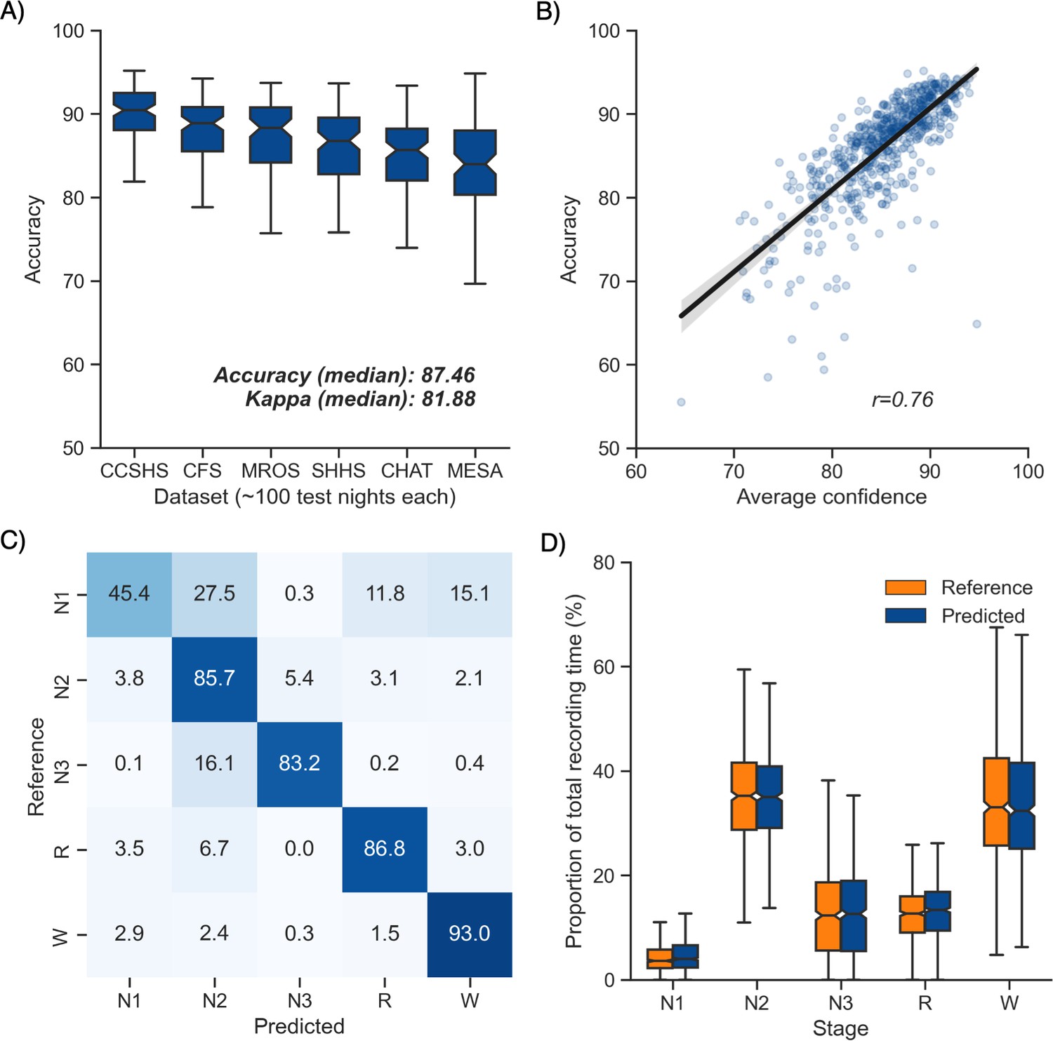
Performance of the algorithm on the testing set 1 (n = 585 nights).
(A) Accuracy of all the testing nights, stratified by dataset. The median accuracy across all testing nights was 87.5%. (B) Correlation between accuracy and average confidence levels (in %) of the algorithm. The overall confidence was calculated for each night by averaging the confidence levels across all epochs. (C) Confusion matrix. The diagonal elements represent the percentage of epochs that were correctly classified by the algorithm (also known as sensitivity or recall), whereas the off-diagonal elements show the percentage of epochs that were mislabeled by the algorithm. (D) Duration of each stage in the human (red) and automatic scoring (green), calculated for each unique testing night and expressed as a proportion of the total duration of the polysomnography (PSG) recording.
Figure 1—figure supplement 1
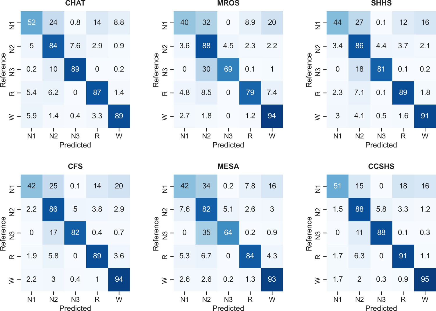
Confusion matrices of the testing set 1, stratified by dataset.
The diagonal elements of the confusion matrices represent the percentage of epochs that were correctly classified by the algorithm (also known as sensitivity or recall), whereas the off-diagonal elements show the percentage of epochs that were mislabeled by the algorithm.
Figure 1—figure supplement 2

Distribution of confidence scores across sleep stages in the testing set 1.
The percent of epochs that were flagged as high-confidence (≥ 80%) by the algorithm was 86.3% for wakefulness (out of a total of 253,471 epochs), 17.5% for N1 (n = 32,783), 62.4% for N2 sleep (n = 249,055), 72.1% for N3 sleep (n = 91,712), and 66.9% for rapid eye movement (REM) sleep (n = 89,346).
Figure 1—figure supplement 3
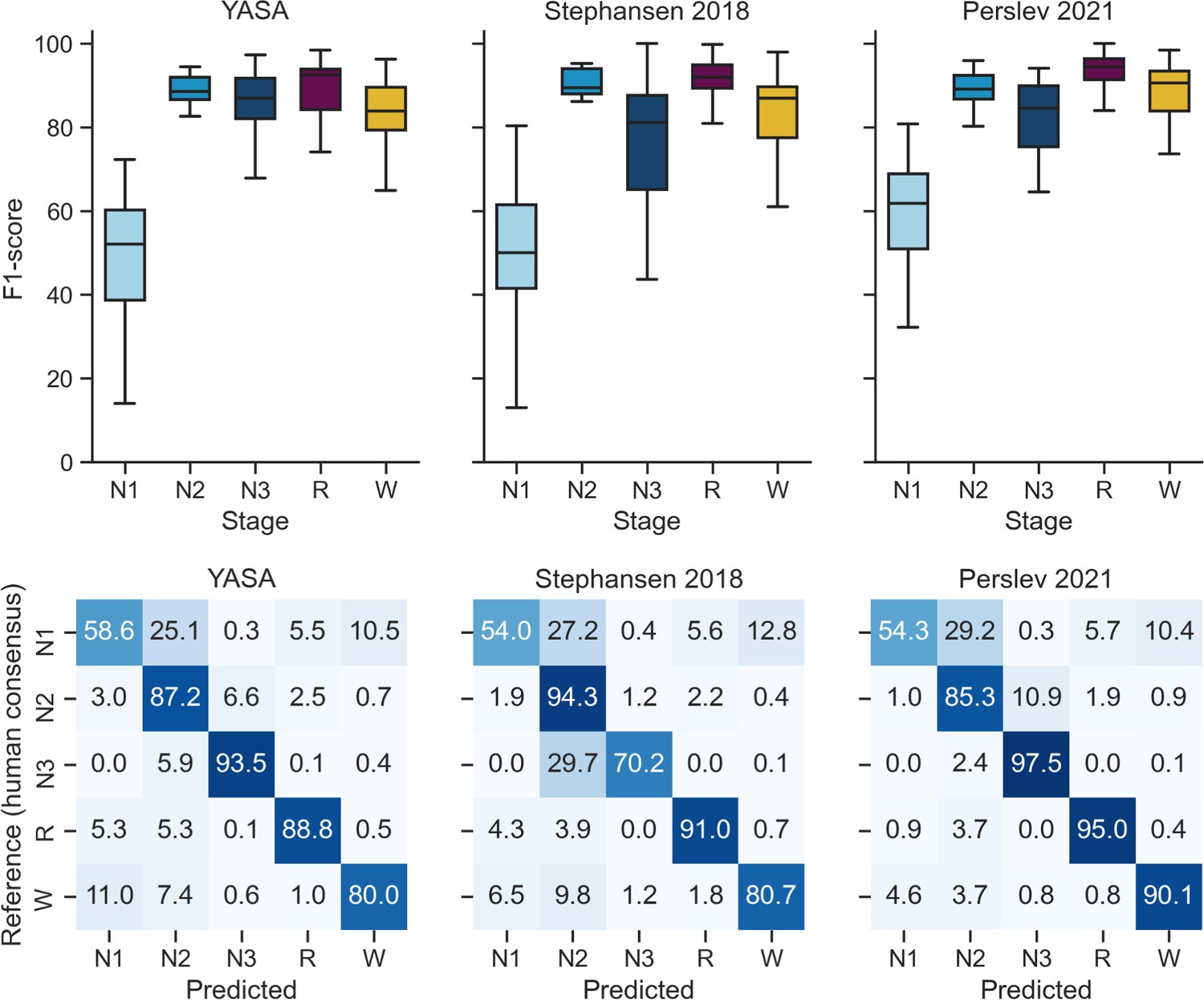
Performance of the YASA, Stephansen et al., 2018, and Perslev et al., 2021 algorithms on the DOD-Healthy testing set (n = 25 healthy adults).
Top, F1-scores. Bottom, confusion matrices. The diagonal elements represent the percentage of epochs that were correctly classified by the algorithm (also known as sensitivity or recall), whereas the off-diagonal elements show the percentage of epochs that were mislabeled by the algorithm.
Figure 1—figure supplement 4
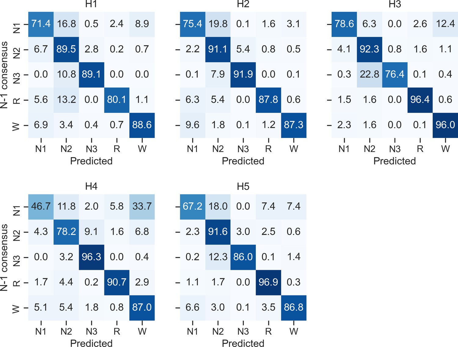
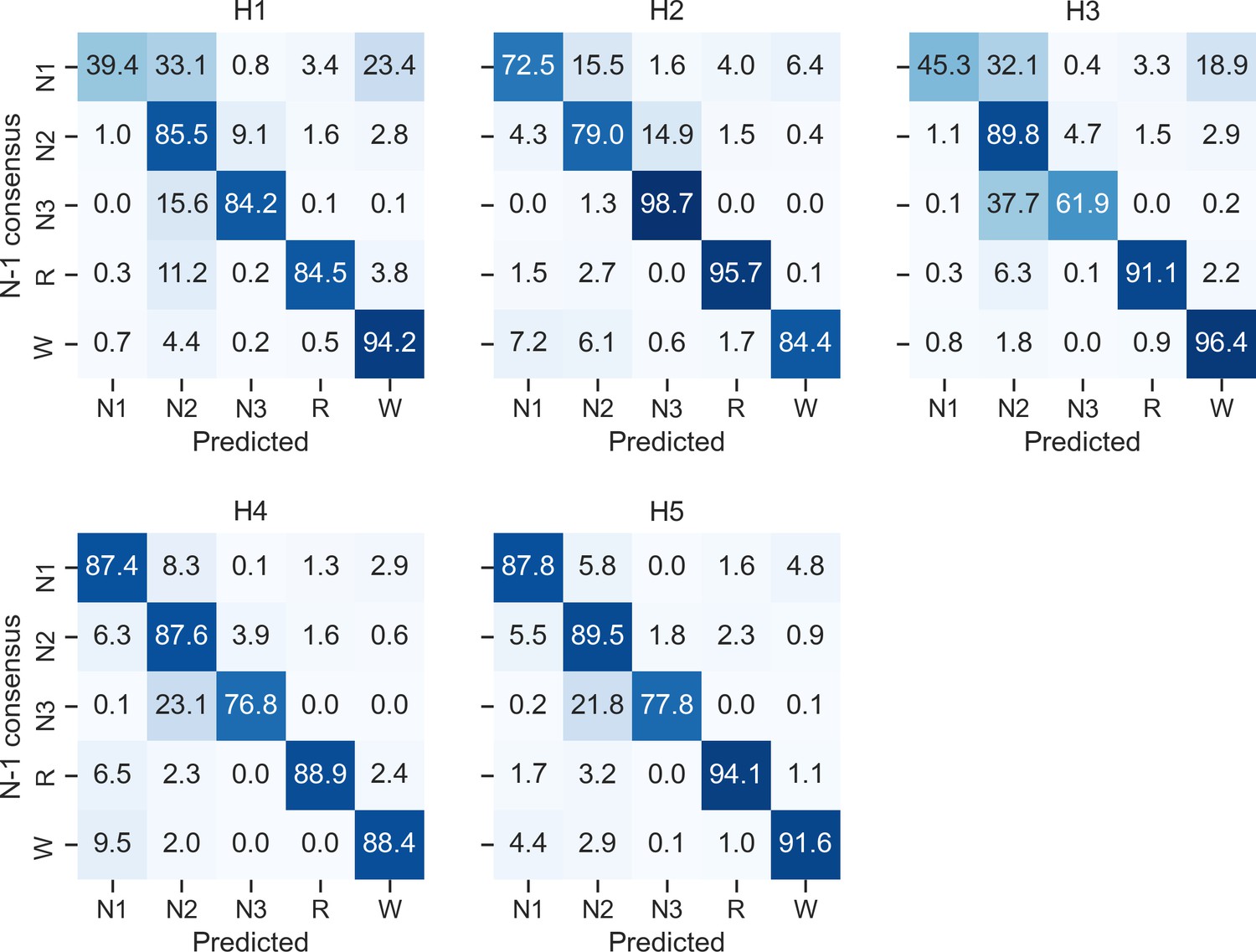
Confusion matrices of each individual human scorer on the DOD-Healthy testing set (n = 25 healthy adults).
Ground truth was defined as the unbiased consensus scoring, that is, excluding the current scorer (see Materials and methods). The diagonal elements of the confusion matrices represent the percentage of epochs that were correctly classified by the human scorer (also known as sensitivity or recall), whereas the off-diagonal elements show the percentage of epochs that were mislabeled by the human scorer.
Figure 1—figure supplement 5

Performance of the YASA, Stephansen et al., 2018, and Perslev et al., 2021 algorithms on the DOD-Obstructive testing set (n = 50 patients with obstructive sleep apnea).
Top, F1-scores. Bottom, confusion matrices. The diagonal elements represent the percentage of epochs that were correctly classified by the algorithm (also known as sensitivity or recall), whereas the off-diagonal elements show the percentage of epochs that were mislabeled by the algorithm.
Figure 1—figure supplement 6
Confusion matrices of each individual human scorer on the DOD-Obstructive testing set (n = 50 patients with sleep apnea).
Ground truth was defined as the unbiased consensus scoring, that is, excluding the current scorer (see Materials and methods). The diagonal elements of the confusion matrices represent the percentage of epochs that were correctly classified by the human scorer (also known as sensitivity or recall), whereas the off-diagonal elements show the percentage of epochs that were mislabeled by the human scorer.
Figure 1—figure supplement 7

Top 20 most important features of the classifier.
The algorithm uses three different versions of all time-domain and frequency-domain features: (1) the raw feature, expressed in the original unit of data and calculated for each 30-sec epoch, (2) a smoothed and normalized version of that feature using a 7.5 min triangular-weighted rolling average, and (3) a smoothed and normalized version of that feature using a past 2 min rolling average. Importance was measured on the full training set during model training using Shapley values (SHAP).
Figure 2
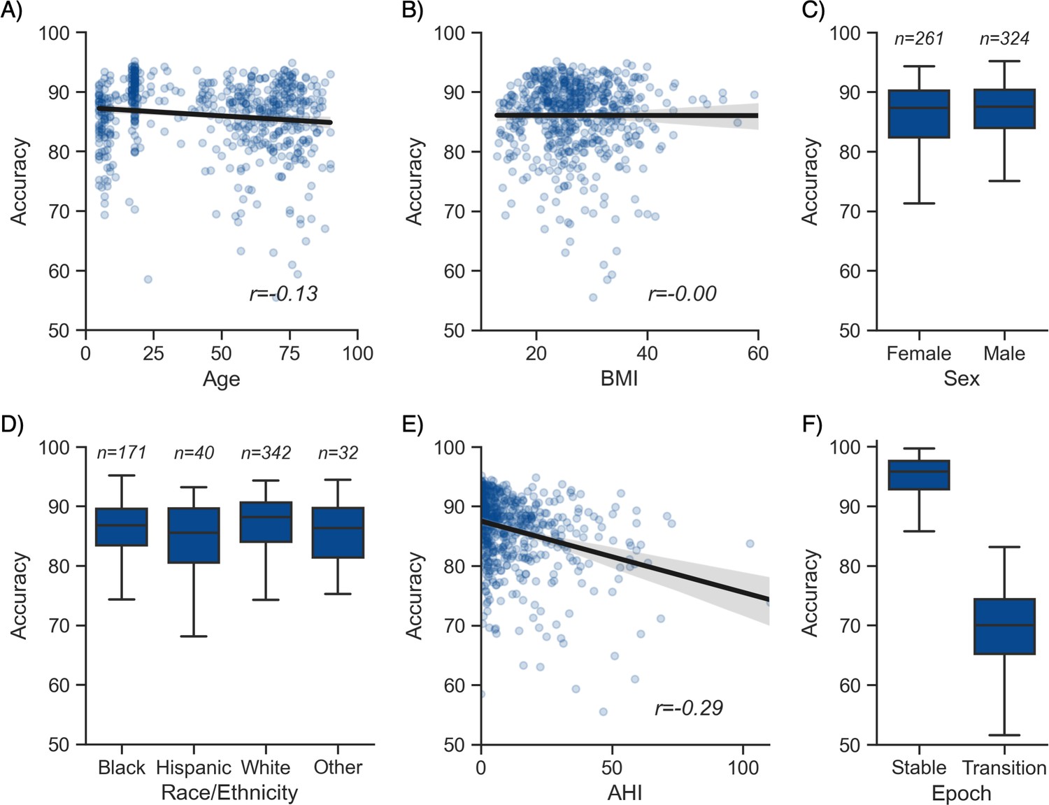
Moderator analyses.
Accuracy of the testing nights as a function of age (A), body mass index (BMI) (B), sex (C), race (D), apnea-hypopnea index (AHI) (E), and whether or not the epoch is around a stage transition (F). An epoch is considered around a transition if a stage transition, as defined by the human scoring, is present within the 3 min around the epoch (1.5 min before, 1.5 min after).
Figure 3 with 2 supplements
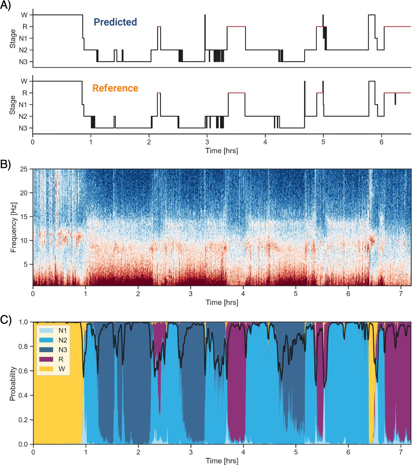
Example of data and sleep stages prediction in one subject.
(A) Predicted and ground-truth ( = human-scored) hypnogram in a healthy young female (CFS dataset, 24 years old, Black, apnea-hypopnea index [AHI] < 1). The agreement between the two scoring is 94.3%. (B) Corresponding full-night spectrogram of the central electroencephalogram (EEG) channel. Warmer colors indicate higher power in these frequencies. This type of plot can be used to easily identify the overall sleep architecture. For example, periods with high power in frequencies below 5 Hz most likely indicate deep non-rapid eye movement (NREM) sleep. (C) Algorithm’s predicted cumulative probabilities of each sleep stage at each 30 s epoch. The black line indicates the confidence level of the algorithm. Note that all the plots in this figure can be very easily plotted in the software.
Figure 3—figure supplement 1

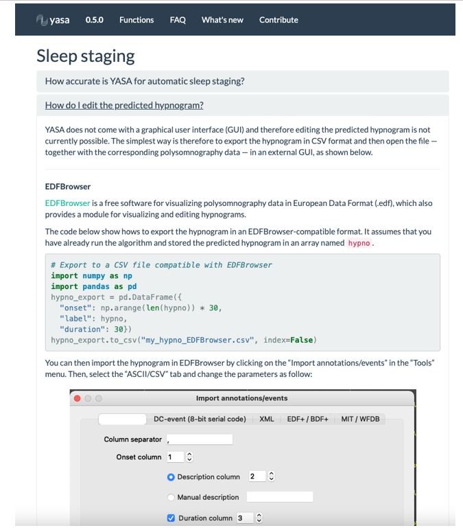
Code snippet illustrating the simplest usage of the algorithm.
Here, automatic sleep staging is applied on an European Data Format (EDF) file, previously loaded using the MNE package. The sleep stages predictions are made using one electroencephalogram (EEG), one electrooculogram (EOG), and one electromyogram (EMG), as well as the age and sex of the participant. The full hypnogram is then exported into a CSV file, together with the epoch number.
Figure 3—figure supplement 2

Code snippet illustrating the usage of the algorithm on multiple European Data Format (EDF) files.
Automatic sleep staging is applied on a batch of EDF files that are present in the same folder. The sleep stages predictions are made using one electroencephalogram (EEG), one electrooculogram (EOG), and one electromyogram (EMG), which are assumed to be consistent across all the polysomnography recordings. The full predicted hypnogram of each recording is then exported into a CSV file with the same filename as the corresponding EDF file.
Author response image 1

Author response image 2
Tables
Table 1
Demographics of the training set and testing set 1.
Age, body mass index (BMI), and apnea-hypopnea index (AHI) are expressed in mean ± standard deviation. The p-value for these three variables was calculated using a Welch’s two-sided t-test, and the effect size refers to the Hedges g. All the other categorical variables are expressed in percentage. Significance was assessed using a chi-square test of independence, and effect size refers to the Cramer’s V. The apnea severity was classified as follows: none = AHI < 5 per hour, mild = AHI ≥ 5 but < 15, moderate = AHI ≥ 15 but < 30, and severe = AHI ≥ 30. p-Values were not adjusted for multiple comparisons.
| Training | Testing set 1 | p-Value | Effect size | |
|---|---|---|---|---|
| No. nights | 561 | 3163 | - | - |
| Age | 49.79 ± 26.38 | 45.25 ± 28.18 | <0.001 | 0.170 |
| BMI | 27.65 ± 7.40 | 26.83 ± 7.30 | 0.013 | 0.111 |
| Sex (% male) | 56.56 | 55.385 | 0.630 | 0.008 |
| Race (%) | - | - | 0.985 | 0.006 |
| Black | 29.47 | 29.23 | - | - |
| White | 57.92 | 58.46 | - | - |
| Hispanic | 7.24 | 6.84 | - | - |
| Asian or Pacific Islander | 5.375 | 5.47 | - | - |
| AHI (events/hour) | 12.94 ± 16.35 | 11.99 ± 14.99 | 0.166 | 0.059 |
| Apnea severity | - | - | 0.820 | 0.016 |
| None | 42.78 | 43.76 | - | - |
| Mild | 27.79 | 27.18 | - | - |
| Moderate | 17.325 | 18.12 | - | - |
| Severe | 12.11 | 10.94 | - | - |
| Insomnia (%) | 6.95 | 4.50 | 0.255 | 0.019 |
| Depression (%) | 15.83 | 13.158 | 0.407 | 0.014 |
| Diabetes (%) | 15.82 | 17.99 | 0.260 | 0.018 |
| Hypertension (%) | 38.83 | 35.27 | 0.152 | 0.023 |
Table 2
Comparison of YASA against two existing algorithms and individual human scorers on the DOD-Healthy dataset (healthy adults, n = 25).
Values represent median ± interquartile range across all n = 25 nights. The YASA column shows the performance of the current algorithm against the consensus scoring of the five human experts (see Materials and methods). The Stephansen et al., 2018 and Perslev et al., 2021 columns show the performance of two recent deep-learning-based sleep-staging algorithms (Perslev et al., 2021; Stephansen et al., 2018). The H1–H5 columns show the performance of each individual human scorer against an unbiased consensus (see Materials and methods). Asterisks indicate significant differences with YASA. p-Values were adjusted for multiple comparisons row-wise using the Holm method. Accuracy is defined as the overall agreement between the predicted and ground-truth sleep stages. F1 is the F1-score, calculated separately for each sleep stage. F1-macro is the average of the F1-scores of all sleep stages.
| YASA | Stephansen et al., 2018 | Perslev et al., 2021 | H1 | H2 | H3 | H4 | H5 | |
|---|---|---|---|---|---|---|---|---|
| Accuracy | 86.6 ± 6.2 | 86.4 ± 5.5 | 89.0 ± 4.8 | 86.5 ± 7.9 | 86.3 ± 5.9 | 86.6 ± 5.9 | 78.8 ± 9.2* | 86.3 ± 7.2 |
| F1 N1 | 52.0 ± 21.6 | 50.0 ± 19.9 | 61.8 ± 18.0* | 50.0 ± 12.2 | 53.7 ± 18.1 | 53.2 ± 19.8 | 38.7 ± 22.1* | 51.7 ± 19.2 |
| F1 N2 | 88.5 ± 5.3 | 89.5 ± 6.0 | 89.1 ± 5.7 | 89.1 ± 5.6 | 88.4 ± 6.0 | 88.1 ± 6.6 | 83.3 ± 5.2* | 88.3 ± 6.2 |
| F1 N3 | 87.0 ± 9.7 | 81.1 ± 22.5 | 84.6 ± 14.6 | 86.9 ± 17.2 | 81.4 ± 18.2 | 82.1 ± 20.6 | 82.5 ± 20.3 | 84.0 ± 11.7 |
| F1 REM | 92.6 ± 9.7 | 91.9 ± 5.6 | 94.4 ± 5.1* | 88.0 ± 13.3 | 90.6 ± 5.5 | 92.7 ± 7.0* | 90.0 ± 9.2 | 92.7 ± 8.1 |
| F1 WAKE | 83.9 ± 10.3 | 87.0 ± 12.2 | 90.5 ± 9.5* | 83.7 ± 9.5 | 87.4 ± 12.0 | 85.7 ± 9.2 | 78.1 ± 28.9 | 84.4 ± 16.8 |
| F1 macro | 78.5 ± 9.4 | 79.0 ± 8.5 | 82.7 ± 7.7* | 78.0 ± 9.0 | 80.0 ± 9.1 | 79.5 ± 7.6 | 73.0 ± 9.0* | 79.5 ± 11.9 |
Table 3
Comparison of YASA against two existing algorithms and individual human scorers on the DOD-Obstructive dataset (patients with obstructive sleep apnea, n = 50).
Values represent median ± interquartile range across all n = 50 nights. The YASA column shows the performance of the current algorithm against the consensus scoring of the five human experts (see Materials and methods). The Stephansen et al., 2018 and Perslev et al., 2021 columns show the performance of two recent deep-learning-based sleep-staging algorithms (Perslev et al., 2021; Stephansen et al., 2018). The H1–H5 columns show the performance of each individual human scorer against an unbiased consensus (see Materials and methods). Asterisks indicate significant differences with YASA. p-Values were adjusted for multiple comparisons row-wise using the Holm method. Accuracy is defined as the overall agreement between the predicted and ground-truth sleep stages. F1 is the F1-score, calculated separately for each sleep stage. F1-macro is the average of the F1-scores of all sleep stages.
| YASA | Stephansen et al., 2018 | Perslev et al., 2021 | H1 | H2 | H3 | H4 | H5 | |
|---|---|---|---|---|---|---|---|---|
| Accuracy | 84.30 ± 7.85 | 84.97 ± 9.48 | 86.69 ± 8.69* | 83.94 ± 12.72 | 82.51 ± 9.49* | 80.38 ± 11.99 | 82.18 ± 9.26 | 84.50 ± 9.78 |
| F1 N1 | 39.17 ± 18.17 | 41.48 ± 17.05 | 50.17 ± 21.17* | 34.44 ± 19.93 | 40.53 ± 29.96 | 39.01 ± 19.78 | 41.54 ± 21.04 | 46.19 ± 20.07* |
| F1 N2 | 87.10 ± 6.55 | 88.36 ± 9.39 | 87.26 ± 8.77 | 86.80 ± 15.96* | 83.07 ± 7.19* | 83.39 ± 11.34 | 84.63 ± 7.57 | 87.29 ± 8.45 |
| F1 N3 | 77.88 ± 31.12 | 57.16 ± 82.16* | 79.51 ± 31.28 | 71.51 ± 56.26* | 65.53 ± 45.41* | 49.97 ± 63.95* | 62.69 ± 61.22* | 74.74 ± 41.19 |
| F1 REM | 88.87 ± 10.79 | 92.50 ± 7.81 | 93.90 ± 5.40* | 89.86 ± 19.43 | 92.48 ± 9.91 | 91.26 ± 12.21 | 89.26 ± 9.83 | 91.77 ± 11.28 |
| F1 WAKE | 86.90 ± 8.47 | 87.95 ± 9.04 | 91.04 ± 8.31* | 90.80 ± 10.00 | 88.48 ± 12.60 | 88.80 ± 11.62 | 90.13 ± 8.90 | 91.06 ± 9.59* |
| F1 macro | 73.96 ± 10.79 | 70.11 ± 15.54 | 78.70 ± 10.90* | 70.91 ± 19.29 | 72.99 ± 15.65 | 68.25 ± 16.22* | 70.43 ± 18.02 | 76.20 ± 16.36 |
Additional files
-
Supplementary file 1
Predictions of the automated algorithms for each night of the DOD-Healthy validation dataset.
Accuracy refers to the percentage of agreement of the algorithm against the human consensus scoring. Nights are ranked in descending order of agreement between YASA and the consensus scoring.
- https://cdn.elifesciences.org/articles/70092/elife-70092-supp1-v1.pdf
-
Supplementary file 2
Predictions of the automated algorithms for each night of the DOD-Obstructive validation dataset.
Accuracy refers to the percentage of agreement of the algorithm against the human consensus scoring. Nights are ranked in descending order of agreement between YASA and the consensus scoring.
- https://cdn.elifesciences.org/articles/70092/elife-70092-supp2-v1.pdf
-
Supplementary file 3
(A) Cross-validation of the best time length for the temporal smoothing of the features.
A total of 49 combinations of past and centered rolling windows were tested, defined as the Cartesian product of the following time lengths for the past rolling average: [none, 1 min, 2 min, 3 min, 5 min, 7 min, 9 min] and the centered rolling weighted average: [none, 1.5 min, 2.5 min, 3.5 min, 5.5 min, 7.5 min, 9.5 min], where none indicates that no rolling window was applied. Cross-validation was performed using a threefold validation on the full training set, stratified by nights, such that a polysomnography (PSG) night was either present in the training and validation set, but never in both at the same time. For speed, only 50 trees were used in the classification algorithm. The ‘Mean’ column is the average of the accuracy and the five F1-scores. Note that the second best-ranked combination (9.5 min centered) has a slightly higher mean score; however, we chose to use a 7.5 min centered window (rank 1) in our final model because it had higher F1-scores for N2, N3, and rapid eye movement (REM) sleep. (B) Contributors of variability in accuracy. Relative importance (%) was estimated with a random forest on n = 585 nights from the testing set 1. The outcome variable of the model was the accuracy score of YASA against ground-truth sleep staging, calculated separately for each night.
- https://cdn.elifesciences.org/articles/70092/elife-70092-supp3-v1.docx
-
Supplementary file 4
All the features are calculated for each consecutive 30 s epoch across the night, starting from the first sample of the polysomnography recording.
Importantly, the algorithm uses three different versions of all time-domain and frequency-domain features: (1) the raw feature, expressed in the original unit of data (e.g., µV for the standard deviation and interquartile range), (2) a smoothed and normalized version of that feature using a 7.5 min triangular-weighted rolling average, and (3) a smoothed and normalized version of that feature using a past 2 min rolling average. Normalization is done after smoothing on a per-night basis with a robust method based on the 5–95% percentiles. Frequency-domain features are based on a Welch’s periodogram with a 5 s window (= 0.2 Hz resolution).
- https://cdn.elifesciences.org/articles/70092/elife-70092-supp4-v1.docx
-
Transparent reporting form
- https://cdn.elifesciences.org/articles/70092/elife-70092-transrepform1-v1.docx
Download links
A two-part list of links to download the article, or parts of the article, in various formats.
Downloads (link to download the article as PDF)
Open citations (links to open the citations from this article in various online reference manager services)
Cite this article (links to download the citations from this article in formats compatible with various reference manager tools)
An open-source, high-performance tool for automated sleep staging
eLife 10:e70092.
https://doi.org/10.7554/eLife.70092


