An open-source, high-performance tool for automated sleep staging

Version of Record

Accepted for publication after peer review and revision.

Download
Cite
Share
CommentOpen annotations (there are currently 0 annotations on this page).

Version of Record published: October 14, 2021 (This version)
Accepted: September 29, 2021
Preprint posted: May 28, 2021 (Go to version)
Received: May 6, 2021

1. Of interest
Translation of dipeptide repeat proteins in C9ORF72 ALS/FTD through unique and redundant AUG initiation codons

Yoshifumi Sonobe, Soojin Lee ... Paschalis Kratsios

Research Article Sep 29, 2023
Further reading

Abstract
Introduction
Results
Discussion
Materials and methods
Data availability
References
Decision letter
Author response
Article and author information
Metrics

Abstract

The clinical and societal measurement of human sleep has increased exponentially in recent years. However, unlike other fields of medical analysis that have become highly automated, basic and clinical sleep research still relies on human visual scoring. Such human-based evaluations are time-consuming, tedious, and can be prone to subjective bias. Here, we describe a novel algorithm trained and validated on +30,000 hr of polysomnographic sleep recordings across heterogeneous populations around the world. This tool offers high sleep-staging accuracy that matches human scoring accuracy and interscorer agreement no matter the population kind. The software is designed to be especially easy to use, computationally low-demanding, open source, and free. Our hope is that this software facilitates the broad adoption of an industry-standard automated sleep staging software package.

Introduction

Sleep is fundamental to human health. Adequate sleep supports a panoply of physiological body functions, including immune, metabolic, and cardiovascular systems (Besedovsky et al., 2019; Cappuccio and Miller, 2017; Harding et al., 2020). Within the brain, sufficient sleep facilitates optimal learning, memory, attention, mood, and decision-making processes (Ben Simon et al., 2020; Walker, 2009). Improving sleep health has therefore emerged as a preventive strategy to reduce the risk of cardiovascular and metabolic disease, all-cause mortality risk, and more recently, the accumulation of Alzheimer’s disease pathology within the brain (Cappuccio et al., 2010; Leary et al., 2020 Cappuccio and Miller, 2017; Ju et al., 2014; Winer et al., 2020). Considering this impact, the demand for quantifying human sleep at a research-, clinical-, and consumer-based level has increased expeditiously over the past decade (Fleming et al., 2015; Shelgikar et al., 2016).

Polysomnography (PSG) – the simultaneous measurement of brainwaves, eye movements, muscle activity, heart rate, and respiration – is the gold standard for objective physiological quantification of human sleep. The classification of sleep stages across the night provides information on the overall architecture of sleep across the night, as well as the duration and proportion of the sleep stages, all of which inform the diagnosis of sleep disorders and specific diseases states.

Currently, such sleep scoring is typically performed by humans, accomplished by first dividing the night of PSG recording into 30 s segments (called ‘epochs’). Each epoch is then assigned a sleep stage based on standard rules defined by the American Academy of Sleep Medicine (AASM, Berry et al., 2012; Iber et al., 2007).

Every night, thousands of hours of sleep are recorded in research, clinical, and commercial ventures across the globe. However, since sleep staging is performed visually by human experts, it represents a pragmatic bottleneck. It is a non-trivial, time-intensive process, with visual scoring of a single night of human sleep requiring up to 2 hr to complete by a well-trained individual. As if not more critical, this human-scored approach suffers from issues of lower than desirable interscorer consistency of agreement (~83% agreement, Rosenberg and Van Hout, 2013). Moreover, the same scoring individual typically experiences low intrascorer agreement of the same sleep recording (~90%, Fiorillo et al., 2019). That is, different human sleep-scoring experts presented with the same recording will likely end up with somewhat dissimilar sleep-staging evaluations, and even the same expert presented with the same recording assessed at two different time points will arrive at differing results.

Advances in machine learning have motivated efforts to try and classify sleep using automated systems. Several such automatic sleep-staging algorithms have emerged in recent years. While an exhaustive review of such sleep-staging algorithms is beyond the scope of this article, we offer an overview of some of the most relevant algorithms within the last 5 years. For a more in-depth review, we refer the reader to Fiorillo et al., 2019.

Sun et al., 2017 reported an algorithm that was trained and evaluated on 2000 PSG recordings from a single-sleep clinic. The overall Cohen’s kappa on the testing set was 0.68 (n = 1000 PSG nights). Thereafter, and algorithm termed ‘Z3Score’ (Patanaik et al., 2018) was published, trained and evaluated on ~1700 PSG recordings from four datasets. Here, the overall accuracy ranged from 89.8% in healthy adults/adolescents to 72.1% in patients with Parkinson’s disease. The freely available ‘Stanford-stage’ algorithm (Stephansen et al., 2018) was trained and evaluated on 10 clinical cohorts (~3000 recordings), and presented with an accuracy of 87% against consensus human sleep stage scoring. A year later, the ‘SeqSleepNet’ algorithm (Phan et al., 2019) was published, which represented a method trained and tested using a 20-fold cross-validation of 200 nights of PSG data, with an overall accuracy of 87.1%. Finally, the recent U-Sleep algorithm (Perslev et al., 2021) was established using PSG recordings from 15,660 participants of 16 clinical studies. The overall accuracy was not reported, though the mean F1-score—a measure reflecting the quality of the prediction against the consensus scoring of five human experts—was 0.79 for healthy adults and 0.76 for patients with sleep apnea.

Despite this growing number of automated tools, accurate automated sleep staging has yet to become a de facto standard in the field. There are likely several reasons for this. First, some algorithms are not free, sitting behind paywalls and/or not publicly available. Second, other algorithms require paid software to run the nonetheless free algorithm on, such as MATLAB. Third, some algorithms have been trained on a sample size too small for robustness and/or data from a single-sleep center or population. As a result, their ability to generalize to other recording systems and/or populations, including patients with sleep disorders or across broad age ranges, has been a concern. Fourth, setting up and running these algorithms is often too complicated for most typical individuals as they require moderate- to high-level programing experience, creating a barrier of entry to adoption and broad use. A final common limitation to all these algorithms is that they were evaluated on different testing datasets and using different metrics, which prevents a direct comparison of the performance of these algorithms and had lead to understandable confusion among some sleep researchers and clinicians.

Seeking to address all such issues, here, we describe a free, flexible, and easy-to-use automated sleep-staging software that has been trained and evaluated on more than 30,000 hr of PSG-staged sleep from numerous independent and heterogeneous datasets with a wide range of age, ethnicities, and health status levels. Furthermore, we test our algorithm against two recent sleep-staging algorithms (Perslev et al., 2021; Stephansen et al., 2018) on a previously unseen consensus-scored sleep dataset of healthy adults and patients with obstructive sleep apnea (OSA).

Results

Descriptive statistics

The training set consisted of more than 31,000 hr of PSG data across 3163 unique full-night PSG recordings from seven different datasets (Cleveland Children’s Sleep and Health Study [CCSHS], n = 414; Cleveland Family Study [CFS], n = 586; Childhood Adenotonsillectomy Trial [CHAT], n = 351; Home Positive Airway Pressure [HomePAP], n = 82; Multi-Ethnic Study of Atherosclerosis [MESA], n = 575; Osteoporotic Fractures in Men Study [MrOS], n = 565; Sleep Heart Health Study [SHHS], n = 590). All these datasets are publicly available from the National Sleep Research Resource (NSRR) website (http://sleepdata.org). In total, these 3163 training nights represent almost 4 million unique 30 s epochs. Demographics and health data of the training set are shown in Table 1. The average apnea-hypopnea index (AHI) was 12.9 ± 16.35 (median = 6.95, range = 0–125). The AHI was ≥15 (= moderate sleep apnea) for 29% of the nights. The MESA dataset had the highest average AHI (19.2 ± 18.1), while the CCSHS had the lowest AHI (1.5 ± 5.2).

Table 1

Demographics of the training set and testing set 1.

Age, body mass index (BMI), and apnea-hypopnea index (AHI) are expressed in mean ± standard deviation. The p-value for these three variables was calculated using a Welch’s two-sided t-test, and the effect size refers to the Hedges g. All the other categorical variables are expressed in percentage. Significance was assessed using a chi-square test of independence, and effect size refers to the Cramer’s V. The apnea severity was classified as follows: none = AHI < 5 per hour, mild = AHI ≥ 5 but < 15, moderate = AHI ≥ 15 but < 30, and severe = AHI ≥ 30. p-Values were not adjusted for multiple comparisons.

	Training	Testing set 1	p-Value	Effect size
No. nights	561	3163	-	-
Age	49.79 ± 26.38	45.25 ± 28.18	<0.001	0.170
BMI	27.65 ± 7.40	26.83 ± 7.30	0.013	0.111
Sex (% male)	56.56	55.385	0.630	0.008
Race (%)	-	-	0.985	0.006
Black	29.47	29.23	-	-
White	57.92	58.46	-	-
Hispanic	7.24	6.84	-	-
Asian or Pacific Islander	5.375	5.47	-	-
AHI (events/hour)	12.94 ± 16.35	11.99 ± 14.99	0.166	0.059
Apnea severity	-	-	0.820	0.016
None	42.78	43.76	-	-
Mild	27.79	27.18	-	-
Moderate	17.325	18.12	-	-
Severe	12.11	10.94	-	-
Insomnia (%)	6.95	4.50	0.255	0.019
Depression (%)	15.83	13.158	0.407	0.014
Diabetes (%)	15.82	17.99	0.260	0.018
Hypertension (%)	38.83	35.27	0.152	0.023

The testing set 1 consisted of 585 unique full-night PSG recordings from six different datasets (CCSHS, n = 100; CFS, n = 99; CHAT, n = 100; MESA, n = 97; MrOS, n = 90; SHHS, n = 99). The testing nights were randomly selected from a subset of nights that were not included in the training set (see Materials and methods). We did not include any nights from the HomePAP dataset because the latter only consisted of 82 nights after preprocessing, all of which were used for training. In total, these 585 testing nights represent 716,367 unique 30 s epochs, or roughly 6000 hr of PSG data. Demographics and health data of the testing set one are shown in Table 1. Importantly, there was no significant difference in the sex ratio, race distribution, or in the proportion of individuals diagnosed with insomnia, depression, or diabetes. Furthermore, there was no difference in AHI and the proportion of individuals with minimal, mild, moderate, or severe sleep apnea. Although participants were randomly assigned in the training/testing sets, there were some significant differences between these two sets. Specifically, age and body mass index (BMI) were lower in the testing set compared to the original training set (p’s<0.05), although the effect sizes of these differences were all below 0.17 (considered small or negligible).

The testing set 2 consisted of 80 full-night PSG recordings from the publicly available Dreem Open Dataset (DOD) dataset (Guillot et al., 2020). The DOD consists of 25 nights from healthy adults (DOD-Healthy: age = 35.3 ± 7.51 years, 76% male, BMI = 23.8 ± 3.4) and 55 nights from patients with OSA (DOD-Obstructive: age = 45.6 ± 16.5 years, 64% male, BMI = 29.6 ± 6.4, AHI = 18.5 ± 16.2). Individual-level demographics and medical history were not provided for the DOD datasets; group averages for age, BMI, and AHI are reported from Guillot et al., 2020. Five nights were excluded because the duration of the PSG data and the duration of the hypnogram differed by more than 1 min, leading to a final sample of 75 nights (~607 hr of data). Each night of the testing set 2 was scored by five registered sleep technicians, thus allowing to test the algorithm against a consensus of human scorers (see Materials and methods). Unlike the NSRR datasets, which were split into training and testing subsets, the two DOD datasets (healthy and patients) were only used for performance evaluation. This provides a more robust estimation of the algorithm’s performance on real-world data from a new sleep clinic or laboratory.

Validation results

Testing set 1: NSRR holdout

Overall performance of the algorithm on the testing set 1 is described in Figure 1A. Median accuracy, calculated across all 585 testing nights, was 87.46%. The median Cohen’s kappa was 0.819, indicating excellent agreement, and similarly, the median Matthews correlation coefficient was 0.821. The CCSHS database testing set had the highest overall accuracy (median = 90.44%), while the MESA database had the lowest accuracy (median = 83.99%). In addition to traditional sleep staging, the algorithm is able to quantify the probability of each sleep stage at each 30 s epoch, which can then be used to derive a confidence score at each epoch. The median confidence of the algorithm across all the testing nights was 85.79%. Nights with a higher average confidence had significantly higher accuracy (Figure 1B, r = 0.76, p<0.001).

Figure 1 with 7 supplements see all

Download asset Open asset

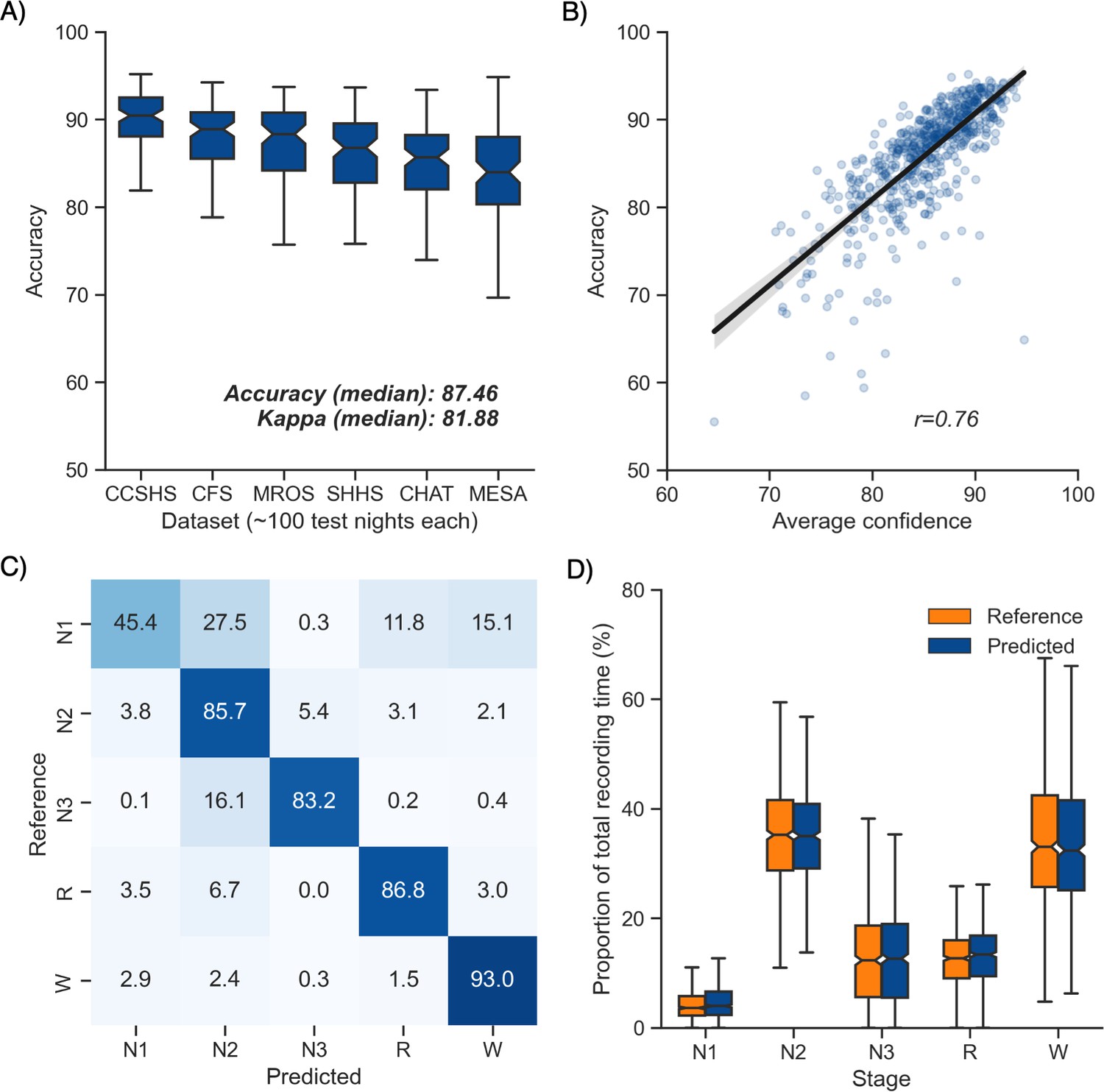
Performance of the algorithm on the testing set 1 (n = 585 nights).

(A) Accuracy of all the testing nights, stratified by dataset. The median accuracy across all testing nights was 87.5%. (B) Correlation between accuracy and average confidence levels (in %) of the algorithm. The overall confidence was calculated for each night by averaging the confidence levels across all epochs. (C) Confusion matrix. The diagonal elements represent the percentage of epochs that were correctly classified by the algorithm (also known as sensitivity or recall), whereas the off-diagonal elements show the percentage of epochs that were mislabeled by the algorithm. (D) Duration of each stage in the human (red) and automatic scoring (green), calculated for each unique testing night and expressed as a proportion of the total duration of the polysomnography (PSG) recording.

Next, we tested the classification performance of individual sleep stages (Figure 1C). The overall sensitivity (i.e., the percent of epochs that were correctly classified, see Materials and methods) of N3 sleep was 83.2%, leading to a median F1-score across all testing nights of 0.835. Rapid eye movement (REM) sleep, N2 sleep, and wakefulness all showed sensitivities above 85% (all median F1-scores ≥ 0.86). N1 sleep showed the lowest agreement, with an overall sensitivity of 45.4% and a median F1-score of 0.432 – a finding consistent with this sleep stage often showing very low agreement across human sleep scorers (<45%, Malhotra et al., 2013). These algorithm performance results were consistent when examined separately for each database (Figure 1—figure supplement 1).

Further examination of the confusion matrix showed that the two most common inaccuracies of the algorithm were (1) mislabeling N1 sleep as N2 sleep (27.5% of all true N1 sleep epochs) and (2) mislabeling N3 sleep as N2 sleep (16.1% of all true N3 sleep epochs). Importantly, the algorithm made few blatant errors, such as mislabeling N3 sleep as REM sleep (0.2%) or mislabeling REM sleep as N3 sleep (0.03%). In addition, when the algorithm misclassified an epoch, the second highest probability stage predicted by the algorithm was the correct one in 76.3% ± 12.6% of the time.

Additional analyses indicated that the algorithm was more prone to inaccuracies around sleep-stage transitions than during stable epochs (Figure 2F; mean accuracy around a stage transition: 69.15% ± 7.23%, during stable periods: 94.08% ± 5.61%, p<0.001). Similarly, and as expected, accuracy was significantly greater for epochs flagged by the algorithm as high confidence (≥80% confidence) than in epochs with a confidence below 80% (95.90% ± 3.70% and 62.91% ± 6.6%, respectively, p<0.001). The distribution of confidence levels across sleep stages is shown in Figure 1—figure supplement 2. The algorithm was most confident in epochs scored as wakefulness by the human scorer (mean confidence across all epochs = 92.7%) and least confident in epochs scored as N1 sleep (mean = 63.2%).

Figure 2

Download asset Open asset

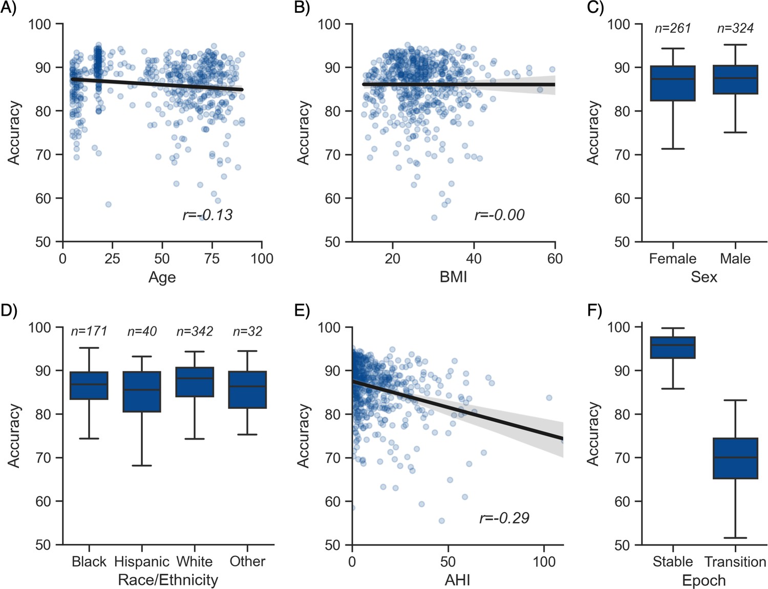
Moderator analyses.

Accuracy of the testing nights as a function of age (A), body mass index (BMI) (B), sex (C), race (D), apnea-hypopnea index (AHI) (E), and whether or not the epoch is around a stage transition (F). An epoch is considered around a transition if a stage transition, as defined by the human scoring, is present within the 3 min around the epoch (1.5 min before, 1.5 min after).

We further tested for any systematic bias of the algorithm towards one or more sleep stages. The overall proportion of each sleep stage in the testing nights was similar between the human and automatic staging (all Cohen’s d < 0.11; Figure 1D), indicating a negligible bias. Similarly, the percentage of stage transitions across the night was consistent in the human and automatic scoring (mean ± STD: 11.12% ± 5.19% and 11.46% ± 4.11%, respectively, Cohen’s d = 0.07).

Testing set 2: Consensus scoring on the DOD-Healthy and DOD-Obstructive datasets

Next, we examined the performance of YASA on the testing set 2, a previously unseen dataset of healthy and sleep-disordered breathing patients that was scored by five registered experts (Guillot et al., 2020; Perslev et al., 2021). Performance of the algorithm is reported in Table 2 for healthy adults (n = 25) and Table 3 for individuals with sleep disorders.

Table 2

Comparison of YASA against two existing algorithms and individual human scorers on the DOD-Healthy dataset (healthy adults, n = 25).

Values represent median ± interquartile range across all n = 25 nights. The YASA column shows the performance of the current algorithm against the consensus scoring of the five human experts (see Materials and methods). The Stephansen et al., 2018 and Perslev et al., 2021 columns show the performance of two recent deep-learning-based sleep-staging algorithms (Perslev et al., 2021; Stephansen et al., 2018). The H1–H5 columns show the performance of each individual human scorer against an unbiased consensus (see Materials and methods). Asterisks indicate significant differences with YASA. p-Values were adjusted for multiple comparisons row-wise using the Holm method. Accuracy is defined as the overall agreement between the predicted and ground-truth sleep stages. F1 is the F1-score, calculated separately for each sleep stage. F1-macro is the average of the F1-scores of all sleep stages.

	YASA	Stephansen et al., 2018	Perslev et al., 2021	H1	H2	H3	H4	H5
Accuracy	86.6 ± 6.2	86.4 ± 5.5	89.0 ± 4.8	86.5 ± 7.9	86.3 ± 5.9	86.6 ± 5.9	78.8 ± 9.2*	86.3 ± 7.2
F1 N1	52.0 ± 21.6	50.0 ± 19.9	61.8 ± 18.0*	50.0 ± 12.2	53.7 ± 18.1	53.2 ± 19.8	38.7 ± 22.1*	51.7 ± 19.2
F1 N2	88.5 ± 5.3	89.5 ± 6.0	89.1 ± 5.7	89.1 ± 5.6	88.4 ± 6.0	88.1 ± 6.6	83.3 ± 5.2*	88.3 ± 6.2
F1 N3	87.0 ± 9.7	81.1 ± 22.5	84.6 ± 14.6	86.9 ± 17.2	81.4 ± 18.2	82.1 ± 20.6	82.5 ± 20.3	84.0 ± 11.7
F1 REM	92.6 ± 9.7	91.9 ± 5.6	94.4 ± 5.1*	88.0 ± 13.3	90.6 ± 5.5	92.7 ± 7.0*	90.0 ± 9.2	92.7 ± 8.1
F1 WAKE	83.9 ± 10.3	87.0 ± 12.2	90.5 ± 9.5*	83.7 ± 9.5	87.4 ± 12.0	85.7 ± 9.2	78.1 ± 28.9	84.4 ± 16.8
F1 macro	78.5 ± 9.4	79.0 ± 8.5	82.7 ± 7.7*	78.0 ± 9.0	80.0 ± 9.1	79.5 ± 7.6	73.0 ± 9.0*	79.5 ± 11.9

Table 3

Comparison of YASA against two existing algorithms and individual human scorers on the DOD-Obstructive dataset (patients with obstructive sleep apnea, n = 50).

Values represent median ± interquartile range across all n = 50 nights. The YASA column shows the performance of the current algorithm against the consensus scoring of the five human experts (see Materials and methods). The Stephansen et al., 2018 and Perslev et al., 2021 columns show the performance of two recent deep-learning-based sleep-staging algorithms (Perslev et al., 2021; Stephansen et al., 2018). The H1–H5 columns show the performance of each individual human scorer against an unbiased consensus (see Materials and methods). Asterisks indicate significant differences with YASA. p-Values were adjusted for multiple comparisons row-wise using the Holm method. Accuracy is defined as the overall agreement between the predicted and ground-truth sleep stages. F1 is the F1-score, calculated separately for each sleep stage. F1-macro is the average of the F1-scores of all sleep stages.

	YASA	Stephansen et al., 2018	Perslev et al., 2021	H1	H2	H3	H4	H5
Accuracy	84.30 ± 7.85	84.97 ± 9.48	86.69 ± 8.69*	83.94 ± 12.72	82.51 ± 9.49*	80.38 ± 11.99	82.18 ± 9.26	84.50 ± 9.78
F1 N1	39.17 ± 18.17	41.48 ± 17.05	50.17 ± 21.17*	34.44 ± 19.93	40.53 ± 29.96	39.01 ± 19.78	41.54 ± 21.04	46.19 ± 20.07*
F1 N2	87.10 ± 6.55	88.36 ± 9.39	87.26 ± 8.77	86.80 ± 15.96*	83.07 ± 7.19*	83.39 ± 11.34	84.63 ± 7.57	87.29 ± 8.45
F1 N3	77.88 ± 31.12	57.16 ± 82.16*	79.51 ± 31.28	71.51 ± 56.26*	65.53 ± 45.41*	49.97 ± 63.95*	62.69 ± 61.22*	74.74 ± 41.19
F1 REM	88.87 ± 10.79	92.50 ± 7.81	93.90 ± 5.40*	89.86 ± 19.43	92.48 ± 9.91	91.26 ± 12.21	89.26 ± 9.83	91.77 ± 11.28
F1 WAKE	86.90 ± 8.47	87.95 ± 9.04	91.04 ± 8.31*	90.80 ± 10.00	88.48 ± 12.60	88.80 ± 11.62	90.13 ± 8.90	91.06 ± 9.59*
F1 macro	73.96 ± 10.79	70.11 ± 15.54	78.70 ± 10.90*	70.91 ± 19.29	72.99 ± 15.65	68.25 ± 16.22*	70.43 ± 18.02	76.20 ± 16.36

In healthy adults, the median accuracy of YASA against the consensus scoring of the five experts was 86.6%. The median kappa across all nights was 80.1%, indicating excellent agreement. Median and interquartile range of F1-scores for each sleep stage across all nights are reported in Table 2. We then compared the performance of YASA against each of the five individual human scorers, as well as against two recently published sleep-staging algorithms (see Materials and methods, Perslev et al., 2021; Stephansen et al., 2018). Pairwise t-tests adjusted for multiple comparisons using the Holm method revealed that the accuracy of YASA on this healthy validation dataset was not significantly different from the two other deep-learning-based sleep-staging algorithms or any of the individual scorers (except scorer 4, see below or Table 2). The F1-scores for each sleep stage were not significantly different between YASA, the Stephansen et al., 2018 algorithm, and the human scorers 1, 2, 3, and 5. Scorer 4 had a significantly lower F1-score for N1 (p=0.034) and N2 (p<0.001), resulting in a lower overall accuracy (p=0.001). The Perslev et al., 2021 algorithm had significantly higher F1-scores than YASA for N1, REM sleep and wakefulness (p=0.006, p<0.001, and p=0.042, respectively). F1-scores for N2 and N3 were not statistically different between YASA and the Perslev et al., 2021 algorithm. Hypnograms of the consensus scoring and the three automated algorithms for each night of the DOD-Healthy dataset can be found in Supplementary file 1, with nights ranked in descending order of agreement between YASA and the consensus scoring. Confusion matrices for each scorer (human and algorithm) can be found in Figure 1—figure supplements 3 and 4.

The same analysis was performed in 55 patients with OSA (DOD-Obstructive). The median accuracy of YASA against the consensus scoring of the five experts was 84.3%, with a median kappa of 76.5%. Median and interquartile range of F1-scores for each sleep stage across all nights are reported in Table 3. Pairwise comparisons of accuracy showed that YASA was not significantly different from the Stephansen et al., 2018 algorithm or human scorers 1, 3, 4, and 5. Human scorer 2 had a significantly lower accuracy (p=0.004), while the Perslev algorithm had a significantly higher accuracy (p=0.009). Pairwise comparisons of F1-scores showed that YASA outperformed the Stephansen et al., 2018 algorithm and four out of five scorers for N3 sleep (all p’s<0.01). However, the Perslev et al., 2021 algorithm had significantly higher scores than YASA for N1, REM and wakefulness (all p’s<0.011). Hypnograms of the consensus scoring and the three automated algorithms, ranked in descending order of agreement between YASA and the consensus scoring, can be found in Supplementary file 2. Confusion matrices are reported in Figure 1—figure supplements 5 and 6.

Additional analyses on the combined dataset (n = 75 nights, healthy and patients combined) revealed that, first, the accuracy of YASA against the consensus scoring was significantly higher during stable epochs compared to transition epochs (mean ± STD: 91.2 ± 7.8 vs. 68.95 ± 7.7, p<0.001), or in epochs that were marked as high confidence by the algorithm (93.9 ± 6.0 vs. 64.1 ± 7.0 for low-confidence epochs, p<0.001). Second, epochs with unanimous consensus from the five human experts were four times more likely to occur during stable epochs than transition epochs (46.2% ± 12.1% of all epochs vs. 11.5% ± 4.9%, p<0.001) and also four times more likely to occur during epochs marked as high confidence (≥80%) by the algorithm (46.4% ± 12.9% of all epochs vs. 11.3% ± 5.7%, p<0.001). Third, there was a significant correlation between the percentage of epochs marked as high confidence by YASA and the percent of epochs with unanimous consensus (r = 0.561, p<0.001), meaning that YASA was overall more confident in recordings with higher human interrater agreement.

Moderator analyses

Having tested the performance of the algorithm on both healthy adults and patients with sleep apnea, we turned our attention to the impact of different moderators on the sleep-staging accuracy. Subsequent analyses are based on the testing set 1 (NSRR), for which – unlike the testing set 2 (DOD) – extensive individual-level demographic and health data was available. As with human sleep scoring, analyses focused on the first factor of age revealed a small but significant negative correlation with accuracy (r = −0.128, p=0.002, Figure 2A), suggesting a moderate linear decrease of accuracy with age. Second, body composition was not significantly correlated with accuracy (r = −0.001, p=0.97, Figure 2B). Third, sex was not a significant determinant of accuracy either (Welch’s T = −1.635, p=0.103, Figure 2C). Fourth, sleep apnea, and specifically the AHI, was negatively correlated with accuracy (r = −0.29, p<0.001, Figure 2E) as well as the overall confidence level of the algorithm (calculated by averaging the epoch-by-epoch confidence across the entire night, r = −0.339, p<0.001). This would indicate that, to a modest degree, the performance and confidence of the algorithm can lessen in those with severe sleep apnea indices, possibly mediated by an increased number of stage transitions in patients with sleep apnea (see above stage transition findings). Consistent with the latter, the percentage of (human-defined) stage transitions was significantly correlated with the AHI (r = 0.427, p<0.001). Finally, race was a significant predictor of accuracy (ANOVA, F(3, 581) = 3.281, p=0.021, Figure 2D). Pairwise post hoc tests adjusted for multiple comparisons with Tukey’s method revealed that accuracy was lower in Hispanic than in non-Hispanic White individuals (p=0.032). However, this effect may be driven by the imbalance in sample size between these two categories (n = 40 vs. n = 342, respectively). No other pairwise comparison between race categories was significant.

To better understand how these moderators influence accuracy variability, we analyzed the relative contribution of the moderators using a random forest analysis. Specifically, we included all the aforementioned demographics variables in the model, together with medical diagnosis of depression, diabetes, hypertension, and insomnia, and features extracted from the ground-truth sleep scoring such as the percentage of each sleep stage, the duration of the recording, and the percentage of stage transitions in the hypnograms. The outcome variable of the model was the accuracy score of YASA against ground-truth sleep staging, calculated separately for each night. All the nights in the testing set 1 were included, leading to a sample size of 585 unique nights. Results are presented in Supplementary file 3b. The percentage of N1 sleep and percentage of stage transitions – both markers of sleep fragmentation – were the two top predictors of accuracy, accounting for 40% of the total relative importance. By contrast, the combined contribution of age, sex, race, and medical diagnosis of insomnia, hypertension, diabetes, and depression accounted for roughly 10% of the total importance.

Features importance

The 20 most important features of the model are shown in Figure 1—figure supplement 7. 11 out of these top 20 features are derived from the electroencephalogram (EEG) signal, 7 from the electrooculogram (EOG), and 1 from the electromyogram (EMG). This indicates that EEG is the most important signal for accurate sleep staging, followed by EOG and to a lesser extent EMG. Time elapsed from the beginning of the recording was also present in the top 20 features, a result consistent with the well-known asymmetry of sleep stages across the night (i.e., more N3 sleep in the first half of the night and more REM sleep in the second half). Consistent with these findings, the algorithm retained high levels of accuracy when using only a single-channel EEG (median accuracy across the 585 nights of the testing set 1 = 85.12%, median kappa = 0.782) or a combination of one EEG and one EOG (median accuracy = 86.92%, median kappa = 0.809). In other words, using only one EEG and one EOG led to an ~0.5% decrease in median accuracy compared to a full model including one EEG, one EOG, one EMG, as well as age and sex.

The single most important feature of the classifier was the absolute power of the EOG power spectrum, followed by the fractal dimension, absolute power, and beta power of the EEG signal. It is relevant that several of these top features are relatively uncommon, nonlinear features (i.e., fractal dimension and permutation entropy). These novel features may capture unique electrophysiological properties of each sleep stage that are missed by traditional linear and/or spectral features. Similarly, 9 out of the 20 most important features include some form of temporal smoothing/normalization (e.g., centered 7.5 min triangular-weighted rolling average). This highlights the importance of taking into account the neighboring epochs – both past and future – for accurate sleep staging (see also Supplementary file 3a).

Software implementation

Implementation of the algorithm is completely open-source and freely available. Our sleep algorithm, colloquially termed YASA (Vallet, 2018) (https://github.com/raphaelvallat/yasa), is part of a broader sleep analysis package (or ‘library’), written in Python. In addition to the automatic sleep-staging module we describe here, YASA also includes several additional functions such as automatic detection of sleep spindles and slow-waves, automatic artifact rejection, calculation of sleep statistics from a hypnogram, spectral power estimation (e.g., Figure 3B), and phase-amplitude coupling. However, use of the basic sleep-staging module is not at all contingent on a desire to quantify any of these metrics. Simply that they are on offer as additional tools in the software suit, should the user wish.

Figure 3 with 2 supplements see all

Download asset Open asset

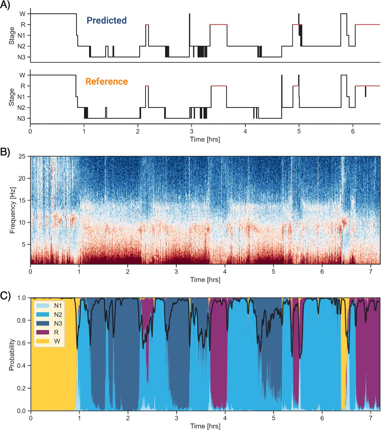
Example of data and sleep stages prediction in one subject.

(A) Predicted and ground-truth ( = human-scored) hypnogram in a healthy young female (CFS dataset, 24 years old, Black, apnea-hypopnea index [AHI] < 1). The agreement between the two scoring is 94.3%. (B) Corresponding full-night spectrogram of the central electroencephalogram (EEG) channel. Warmer colors indicate higher power in these frequencies. This type of plot can be used to easily identify the overall sleep architecture. For example, periods with high power in frequencies below 5 Hz most likely indicate deep non-rapid eye movement (NREM) sleep. (C) Algorithm’s predicted cumulative probabilities of each sleep stage at each 30 s epoch. The black line indicates the confidence level of the algorithm. Note that all the plots in this figure can be very easily plotted in the software.

YASA comes with extensive documentation and is released under a BSD-3 Clause license, part of the Open Source Initiative, and can be directly installed with one simple line of code from the Python Package Index repository (in a terminal: pip install yasa). The source code of YASA is freely and publicly hosted on GitHub, and follows standard release cycles with a version-tracking of all the changes made to the code and/or pretrained classifiers. That is, users can choose to ignore the most recent versions and keep a specific version of the code and staging algorithm, which is useful, for example, in longitudinal studies where the preprocessing and analysis steps should stay consistent across time.

The general workflow to perform the automatic sleep staging is described below. In addition, we provide code snippets showing the simplest usage of the algorithm on a single European Data Format (EDF) file (Figure 3—figure supplement 1) or on a folder with multiple EDF files (Figure 3—figure supplement 2). First, the user loads the PSG data into Python. Assuming that the PSG data are stored in the gold-standard EDF, this can be done in one line of code using the MNE package (Gramfort et al., 2014), which has a dedicated function to load EDF files (https://mne.tools/stable/generated/mne.io.read_raw_edf.html). Second, the automatic sleep staging is performed using the algorithm’s sleep-staging module (https://raphaelvallat.com/yasa/build/html/generated/yasa.SleepStaging.html). The only requirement is that the user specify the name of the EEG channel they want to apply the detection (preferentially a central derivation such as C4-M1). The algorithm is now ready to stage the data. Should the user wish, there is the option of naming EOG and EMG channels (preferentially a chin EMG). The user can also include ancillary if desired, such as age and sex, which can aid in improving the accuracy of the algorithm, though this is not at all necessary for high accuracy (as described earlier).

Regarding the processing steps of the algorithm, sleep staging is performed with the `predict` function. This function automatically identifies and loads the pretrained classifier corresponding to the combination of sensors/metadata provided by the user. While pretrained classifiers are natively included in the algorithm, a user can define custom pretrained classifiers if they wish, which can be tailored to their specific use cases. Once again, however, this is just for flexibility of use and is not at all required for the algorithm to perform with high accuracy. Parenthetically, this flexibility can also be leveraged for a variety of use cases, for example, scoring rodent sleep data instead of human sleep data.

In addition to stage scoring, implementation of the `predict_proba` function provides the ability for a user to quantify the probability certainty of each stage at each epoch. This probability certainty can then be used to derive a confidence score, should that be desired, although again this is not necessary for standard sleep staging by a user (Figure 3C). Finally, the predicted hypnogram and stage probabilities can easily be exported into a text or CSV file using standard Python functions, should the user wish, though once again this is not required.

One limitation of automated data analysis methods is that they are computationally demanding (Fiorillo et al., 2019), often requiring specific higher-end computer systems that are costly. To avoid this limitation, the current algorithm is designed to be fast and highly memory-effective by leveraging high-performance tools in Python (e.g., Numpy’s vectorization and Numba compiling). As a consequence, a full-night PSG recording sampled at 100 Hz is typically processed in less than 5 s on a rudimentary, basic consumer-level laptop.

Discussion

We sought to develop a sleep-staging algorithm that (1) matches human-scorer accuracy, (2) has been trained on a large and heterogeneous data set, (3) is easy to implement by most individuals, (4) is computational low-demanding and can therefore be run on a basic laptop, and (5) is entirely free, and thus easily adopted by researchers, clinicians, and commercial ventures.

Performance

The algorithm displayed high levels of accuracy, matching those observed across human interrater agreement (Fiorillo et al., 2019). First, the median agreement between the algorithm and human scoring across 585 testing nights from the NSRR database was 87.5% – and was superior to 90% when only considering epochs that occurred during a stable period of sleep, that is, not around a stage transition. Second, the performance of YASA was tested on a previously unseen dataset of 25 healthy adults and 50 patients with OSA. Each night of this dataset was scored by five registered experts. The median accuracy of the algorithm against the consensus of the five experts was 86.6% for healthy adults and 84.3% in patients. In both samples, the accuracy of YASA was not significantly different from any of the individual human scorers. Furthermore, comparison against two recent deep-learning algorithms (Stephansen et al., 2018; Perslev et al., 2021) showed that the accuracy of YASA against consensus scoring was on par (i.e., not statistically different) with the two existing algorithms for healthy adults. However, YASA performed worse than the Perslev et al., 2021 algorithm in patients with OSA by 2.4% (as discussed in the ‘Limitations and future directions’ section).

Regarding individual sleep stages, the algorithm showed excellent classification performance for N2 sleep, N3 sleep, REM sleep and wakefulness, and moderate agreement for N1 sleep. These results are consistent with human interrater agreement, which has been found to be consistently lower in N1 sleep compared to the other sleep stages (Malhotra et al., 2013; Norman et al., 2000; Rosenberg and Van Hout, 2013). Furthermore, the algorithm was successful in preserving the overall distribution of sleep stages across the night, such that it is neither over- or underestimating a specific sleep stage.

Beyond a basic sleep-stage classification, an advantage of the algorithm is its ability to provide probability (i.e., likelihood) value for each individual epoch of each stage (Stephansen et al., 2018). These probabilities inform the users about the confidence level of the algorithm. As such, the algorithm provides a unique feature addition for sleep scoring that extends beyond sleep-staging quantification and layers atop sleep-staging qualitative assessment. Proving the validity of this measure, the accuracy of the algorithm was statistically superior in epochs that were flagged as high-confidence, reaching ~95% agreement with human scoring. In addition, recordings with a higher average confidence had significantly higher accuracy. Among many other advantages, such an ability could be used in a semi-supervised scoring approach if desired, wherein a human scorer can focus expressly on the selection of low-confidence epochs and/or recordings for attention, thus limiting time investment.

Generalizability

The power and utility of an algorithm is not just determined by its accuracy, but also by the characteristics of the underlying dataset that was used for training and validation (Fiorillo et al., 2019). For example, an algorithm showing excellent performance but that was trained on a very small and homogeneous sample size (e.g., 10–20 healthy young adults from the same demographic group and recorded using the same device) will typically have low utility for other use cases, such as scoring data from another PSG device, or data from patients with sleep disorders. The generalizability of such algorithms can therefore be compromised, with the high performance most likely indicating overfitting to the small training dataset.

Seeking to avoid this issue, our algorithm was trained and evaluated on more than 30,000 hr of PSG human sleep recordings across almost 4000 nights, from numerous independent and heterogeneous datasets. These datasets included participants from a wide age range, different geographical locations, racial groups, sex, body composition, health status, and sleep disorders. Importantly, these independent studies involved different recording devices and settings (e.g., montage, sampling rate). Such a high heterogeneity is paramount to ensure a high reliability and generalizability of the algorithm.

Moderator analyses showed that the performance of the algorithm was unaffected by sex and body composition. Consistent with human scoring (Muehlroth and Werkle-Bergner, 2020; Norman et al., 2000), the performance of the algorithm was sensitive to advancing age and increasing severity of sleep apnea, although accuracy remained high in patients with sleep apnea (~84% in the DOD-Obstructive validation dataset). The latter two circumstances can be explained by the increase in the number of stage transitions and the increase in the proportion of N1 sleep typically seen in aging and sleep apnea (Norman et al., 2000; Ohayon et al., 2004). Indeed, the majority of such scoring errors were located around stage transitions and/or in N1 sleep, which is consistent with findings of human interrater error of these same circumstances (Norman et al., 2000).

Another problematic challenge in the field of automated sleep staging is the fact that each algorithm is usually tested on a different (often nonpublicly available) dataset, which renders the comparison of algorithms nearly impossible. Adding to this, prior approaches are also heterogeneous in the performance evaluation metrics used to validate the algorithm, as well as in the PSG channel(s) on which the algorithm is applied – with some algorithms using only a single EEG channel and others a multichannel approach (Fiorillo et al., 2019). Addressing these issues, the current algorithm was trained and tested on publicly available datasets, using standard classification metrics (e.g., accuracy, F1-scores, confusion matrix) and following recent guidelines for performance evaluation (Menghini et al., 2021). Furthermore, the built-in flexibility of the algorithm allows for different combinations of channels to be used, should a user wish. For all these reasons, we hope that the algorithm is not only of broad utility, but will facilitate replication of our work and comparison to existing and future works.

Ease-of-use and computationally low demand

To facilitate wide adoption by the sleep community, it is of utmost importance that any algorithm can be used and understood by all parties concerned (e.g., students, researchers, clinicians, technicians), no matter the level of technical expertise. To ensure this, the software has been built with a particular focus on ease-of-use, documentation, and transparency.

First, the end-to-end sleep-staging pipeline can be written in less than 10 lines of Python code, and the software comes with pretrained classifiers that are automatically selected based on the combination of channels used, thus limiting the risk of any error. Second, the software has extensive documentation and includes numerous example datasets, allowing any users to get familiarized with the algorithm before applying it to their own datasets, if they wish (though it is not necessary). Third, the algorithm uses a traditional features-based approach to classify sleep stages instead of a black-box algorithm. These features are described in detail in the documentation and source code of the algorithm, and can be explained to any researchers or clinicians in lay terms. Finally, the sleep staging is done locally on the user’s computer, and the data is never uploaded to the cloud or any external servers, thus limiting security and privacy risks (Fiorillo et al., 2019), and the need for any connectivity when using the software.

Free, open source, and community-driven

Another potential reason that automated sleep staging has yet to become a de facto standard is that some algorithms are sitting behind a paywall (e.g., Malhotra et al., 2013; Patanaik et al., 2018). By contrast, the current algorithm is free and released under a nonrestrictive BSD-3 open-source license. The software, which also includes other sleep analysis tools (e.g., sleep spindle detection, spectral estimation, automatic artifact rejection, phase-amplitude coupling), is hosted on GitHub and has already been downloaded several thousand times at the date of writing (https://static.pepy.tech/badge/yasa). The software can therefore be used by for- or non-profit outlets for free, without constraint.

Limitations and future directions

Despite its numerous advantages, there are limitations to the algorithm that must be considered. These are discussed below, together with ideas for future improvements of the algorithm. First, while the accuracy of YASA against consensus scoring was not significantly different from the Stephansen et al., 2018 and Perslev et al., 2021 algorithms on healthy adults, it was significantly lower than the latter algorithm on patients with OSA. The Perslev et al., 2021 algorithm used all available EEGs and two (bilateral) EOGs, whereas YASA’s scoring was based on one central EEG, one EOG, and one EMG. This suggests that one way to improve performance on this population could be the inclusion of more EEG channels and/or bilateral EOGs. For instance, using the negative product of bilateral EOGs may increase sensitivity to rapid eye movements in REM sleep or slow eye movements in N1 sleep (Agarwal et al., 2005; Stephansen et al., 2018). Interestingly, the Perslev et al., 2021 algorithm does not use an EMG channel, which is consistent with our observation of a negligible benefit on accuracy when adding EMG to the model. This may also indicate that while the current set of features implemented in the algorithm performs well for EEG and EOG channels, it does not fully capture the meaningful dynamic information nested within muscle activity during sleep.

Second, an obstacle to the wide adoption of the current algorithm is the absence of a graphical user interface (GUI). Designing and maintaining an open-source cross-platform GUI is in itself a herculean task that requires dedicated funding and software engineers. Rather, significant efforts have been made to facilitate the integration of YASA’s outputs to existing sleep GUIs. Specifically, the documentation of the algorithm includes examples on how to load and edit the sleep scores in several free GUIs, such as EDFBrowser, Visbrain, and SleepTrip.

Third, the algorithm was exclusively tested and evaluated on full-night PSG recordings. As such, its performance on shorter recordings, such as daytime naps, is unknown. Further testing of the algorithm is therefore required to validate the algorithm on naps. While YASA can process input data of arbitrary length, performance may be reduced on data that are shorter than the longest smoothing windows used by the algorithm (i.e., shorter than 7.5 min).

Fourth, unlike other deep-learning-based algorithms (e.g., Perslev et al., 2021; Stephansen et al., 2018), the algorithm does not currently have the ability to score in shorter resolution. We think however that this is not a significant limitation of our work. First, without exception, all of the datasets used either in the training or testing the current algorithm were visually scored by experts using a 30 s resolution. Therefore, even if our algorithm was able to generate sleep scores in a shorter resolution, comparison against the ground-truth would require downsampling the predictions to a 30 s resolution and thus losing the benefit of the shorter resolution. A proper implementation of a shorter resolution scoring requires to train and validate the model on ground-truth sleep scores of the same temporal resolution. Second, the use of 30 s epochs remains the gold standard (as defined in the most recent version of the AASM manual), and as such, the vast majority of sleep centers across the world still rely on 30 s staging. Provided that datasets with sleep scoring at shorter resolution (e.g., 5, 10, 15 s) becomes common, the current algorithm could be modified and retrained to yield such higher-resolution predictions. In that case, the minimum viable resolution would be 5 s, which is the length of the Fast Fourier Transform used to calculate the spectral powers. That said, we firmly believe that a more temporally fine-grained sleep staging will be of benefit to the sleep community in the future. Indeed, such ‘high-frequency’ staging may improve classification accuracy in error-prone ambiguous epochs (e.g., transition epochs with multiple stages), and has further been shown to better discriminate between healthy and sleep-disordered patients than traditional 30 s-based staging (Perslev et al., 2021).

Fifth, the algorithm is not currently able to identify markers of common sleep disorders (such as sleep apnea, leg movements), and as such may not be suited for clinical purposes. It should be noted however that our software does include several other functions to quantify phasic events during sleep (slow-waves, spindles, REMs, artifacts), as well as sleep fragmentation of the hypnogram. Rather than replacing the crucial expertise of clinicians, YASA may thus provide a helpful starting point to accelerate clinical scoring of PSG recordings. Furthermore, future developments of the software should prioritize automated scoring of clinical disorders, particularly apnea-hypopnea events. On the latter, YASA could implement some of the algorithms that have been developed over the last few years to detect apnea-hypopnea events from the ECG or respiratory channels (e.g., Koley and Dey, 2013; Varon et al., 2015).

A final limitation is that the algorithm is tailored to human scalp data. As such, individuals who may want to use YASA to score intracranial human data, animal data, or even human data from a very specific population will need to adjust the algorithm for their own needs. There are two levels at which the algorithm can be modified. First, an individual may want to retrain the classifier on a specific population without modifying the underlying features. Such flexibility is natively supported by the algorithm and no modifications to the original source code of YASA will be required. However, in some cases, the features may need to be modified as well to capture different aspects and dynamics of the input data (e.g., rodents or human intracranial data). In that case, the users will need to make modifications to the source code of the algorithm, and thus have some knowledge of Python and Git – both of which are now extensively taught in high schools and universities (https://wiki.python.org/moin/SchoolsUsingPython, https://education.github.com/schools). Of note, the entire feature extraction pipeline takes about 100 lines of code and is based on standard scientific Python libraries such as NumPy, SciPy, and Pandas.

Advantages of YASA against existing tools

Although recent advances in artificial intelligence have made it possible to automate tedious tasks in numerous fields of medicine, the sleep research field still relies on human visual scoring, which is time-consuming and can be prone to subjective bias. It is our opinion that one roadblock that has prevented the wide adoption of automatic sleep staging is the sheer number of algorithms that are published each year, most of which are virtually incomparable to others because they use different testing datasets and/or different evaluation strategies. Here, in an effort of transparency, we have benchmarked our algorithm against two of the most significant algorithms that have been published in recent years (Perslev et al., 2021; Stephansen et al., 2018), using exactly the same publicly available dataset. As expected, all three algorithms had high levels of accuracy against consensus scoring, that is, on par with typical human interrater agreement. In addition with its high accuracy, there are unique advantages of YASA that should be considered by potential users, which we describe below.

First, and unlike the vast majority of existing algorithms, YASA was not designed for the sole purpose of staging sleep, but rather as an extensive toolbox encompassing the large majority of all analyses used by sleep researchers and clinicians. This includes, among others, (1) the calculation of sleep statistics from the hypnogram, (2) the automatic detection of phasic events during sleep (such as spindles, slow-waves, REMs, and body movements), (3) spectral analysis, as well as (4) more complex and novel analysis methods that we and others have developed, including event-locked cross-frequency coupling (Helfrich et al., 2018; Staresina et al., 2015) and decomposition of the sleep power spectrum into aperiodic and oscillatory components (Lendner et al., 2020; Wen and Liu, 2016). As such, our software provides an open-source end-to-end framework for the analysis of PSG sleep data, with sleep staging being a (optional) first step in the analysis pipeline.

A second advantage of YASA compared to existing algorithms is processing speed. Indeed, YASA is orders of magnitude faster than the Stephansen et al., 2018 algorithm (~10–20 s vs. 10–20 min, including data loading). Noteworthy, while the Perslev et al., 2021 algorithm is computationally fast, uploading the EDF file to the web server can be slow – in addition to being not adequate for sensitive clinical data. While these differences in processing times may not be problematic for small studies, they can scale dramatically when working with hundreds of recordings.

Third, there are only a limited number of people who have the technical skills and/or required hardware to modify and retrain complex deep-learning neural network architectures, such as the ones implemented in the Perslev et al., 2021 and Stephansen et al., 2018 algorithms. In other words, making changes to these algorithms or adapting them to specific needs is practically unfeasible for the average or even advanced user. By contrast, the core YASA algorithm can be easily modified by someone with such rudimentary knowledge of Python, and the full model can be trained on any basic laptop in no more than a couple of hours. Anecdotally, there are a number of ongoing efforts by other research teams to adapt the algorithm to various needs, such as animal data or human intracranial data. It is therefore our hope that such a simple and easily modifiable architecture may foster collaborative development.

Conclusion

The interest in quantifying and tracking of human sleep has increased exponentially in the past decade (Fleming et al., 2015; Shelgikar et al., 2016), and demand for a highly automated, accurate, high-speed, and easy-to-implement algorithm for the scoring of human sleep has scaled similarly. Here, we offer an algorithm that seeks to accomplish this need. It is our hope that this free tool has the potential for broad adoption across all outlets (research, clinical, commercial) and use cases. With further validation and feedback from the sleep community, we hope it can become an industry standard method, one that can be built upon, expanded, and refined through cross-collaborative open-source community development.

Materials and methods

Datasets

Request a detailed protocol

The algorithm was trained on a collection of large-scale independent datasets from the NSRR ( https://sleepdata.org/; Dean et al., 2016; Zhang et al., 2018) – a web portal funded by the National Heart, Lung and Blood Institute (NHLBI). This database offers access to large collections of deidentified physiological signals and clinical data collected in research cohorts and clinical trials. All data were collected as part of research protocols that were approved by the local institutional review board at each institution, with written and informed consent obtained from each individual before participation. All PSG recordings were scored by trained technicians using standard AASM guidelines (Iber et al., 2007; Silber et al., 2007). A full description of the datasets can be found on https://sleepdataorg/. The following datasets were used.

MESA

Request a detailed protocol

The MESA is a multicenter longitudinal investigation of factors associated with the development of subclinical cardiovascular disease and the progression of subclinical to clinical cardiovascular disease in 6814 Black, White, Hispanic, and Chinese-American men and women initially aged 45–84 at baseline in 2000–2002. Full overnight PSG recordings were collected during the last follow-up visit in 2010–2012 and included 2237 participants (age range = 54–95 years). In-home PSG was conducted using the Compumedics Somte System (Compumedics Ltd., Abbotsford, Australia). The recording montage consisted of three cortical EEG (central C4-M1, occipital Oz-Cz, and frontal Fz-Cz leads), bilateral EOG, chin EMG, as well as several other sensors to measure heart rate, respiration, and leg movements. PSG data were sampled at 256 Hz, and a hardware low-pass filter with a cutoff frequency at 100 Hz was applied during recording.

CFS

Request a detailed protocol

The CFS is a family-based study of sleep apnea, consisting of 2284 individuals (46% African-American) from 361 families studied on up to four occasions over a period of 16 years. We used the full overnight PSG recordings from the last exam (visit 5, n = 735, age range = 6–88 years). In-lab PSG was performed using the Compumedics E-Series System. The recording montage included two cortical EEG (C3-Fpz, C4-Fpz), bilateral EOG, and chin EMG. EEG and EOG channels were sampled at 128 Hz, and EMG was sampled at 256 Hz. A hardware bandpass filter with cutoff frequencies at 0.016 Hz and 105 Hz was applied during recording.

CCSHS

Request a detailed protocol

The CCSHS is a population-based pediatric study with objective sleep evaluation, characterized by a large minority representation. We used the most recent visit, which took place between 2006 and 2010 and included in-lab PSG (n = 517, age range = 16–19 years). The PSG recording (Compumedics E-series, Compumedics) included two cortical EEG (C3-Fpz and C4-Fpz), bilateral EOG, and chin EMG. All channels were sampled at 128 Hz, and a hardware high-pass filter with cutoff frequency at 0.15 Hz was applied during recording.

SHHS

Request a detailed protocol

The SHHS is a multicenter cohort study to determine the cardiovascular and other consequences of sleep-disordered breathing. We only included the first visit, which took place between 1995 and 1998 and included full, in-lab PSG from 5,804 participants (age range = 40–89 years). The PSG recording (Compumedics P-Series, Compumedics) included two cortical EEG (C3-M2 and C4-M1), bilateral EOG, and chin EMG. All channels were sampled at 125 Hz, and a hardware high-pass filter with cutoff frequency at 0.15 Hz was applied during recording.

MrOS

Request a detailed protocol

The MrOS is a multicenter observational study of 5994 men, of which the sleep study is a follow-up ancillary study. Overnight PSG recordings were collected for 2907 participants (age range = 65–89 years), which represents about half of the participants included in the parent study. The PSG recordings (Compumedics P-Series, Compumedics) included two cortical EEG (C3-Fpz and C4-Fpz), bilateral EOG, and chin EMG. All channels were sampled at 256 Hz, and a hardware high-pass filter with cutoff frequency at 0.15 Hz was applied during recording.

CHAT

Request a detailed protocol

The CHAT is a multicenter, single-blind, randomized-controlled trial designed to test whether after a 7-month observation period children, ages 5–9.9 years, with mild to moderate OSA randomized to early adenotonsillectomy will show greater levels of neurocognitive functioning. Overnight PSG recordings were collected between 2007 and 2012 and included 1447 participants (age range = 5–9.9 years), of which 464 were randomized to treatment. The PSG recording consisted of eight cortical EEG (including C3-Fpz and C4-Fpz), bilateral EOG, and chin EMG. All channels were sampled at 200 Hz.

HomePAP

Request a detailed protocol

The HomePAP is a multisite, randomized-controlled trial that enrolled 373 patients (age range = 20–80 years), with a high pretest probability of moderate to severe OSA. We used the in-lab PSG recording, which included six cortical EEG (including C3-Fpz and C4-Fpz), bilateral EOG, and chin EMG. All channels were sampled at 200 Hz.

Each dataset was randomly split into training (up to 600 nights) and testing (up to 100 nights) sets. PSG nights included in the training set were used for model building and training, while PSG nights included in the testing set were used for performance evaluation. Importantly, the training and testing sets were completely separate (i.e., no overlap). The code used to generate the training and testing sets can be found here. Demographics and health data such as the age, sex, race/ethnicity, BMI, AHI (3% desaturation), as well as medical diagnosis of insomnia, depression, diabetes, and hypertension were also provided for each dataset.

To provide an unbiased evaluation of the model on a completely new dataset, we further tested the performance of the algorithm on the DOD (Guillot et al., 2020), a publicly available dataset including healthy individuals (DOD-Healthy) and patients with OSA (DOD-Obstructive).

DOD-Healthy

Request a detailed protocol

The DOD-Healthy consists of 25 healthy volunteers that were enrolled at the French Armed Forces Biomedical Research Institute’s Fatigue and Vigilance Unit in France. Participants were without sleep complaints, aged 18–65, and recruited without regard to gender or ethnicity. PSG recordings were conducted with a Siesta PSG device (Compumedics) and included 12 EEG derivations (C3/M2, F4/M1, F3/F4, F3/M2, F4/O2, F3/O1,FP1/F3, FP1/M2, FP1/O1, FP2/F4, FP2/M1, FP2/O2), 1 EMG and bilateral EOGs, all sampled at 250 Hz.

DOD-Obstructive

Request a detailed protocol

The DOD-Obstructive includes 55 patients with clinical suspicion for sleep-related breathing disorder. PSG was conducted at the Stanford Sleep Medicine Center in the US (clinical trial NCT03657329). Individuals clinically diagnosed with sleep disorders other than OSA, suffering from morbid obesity, taking sleep medications, or with certain cardiopulmonary or neurological comorbidities were excluded from the study. PSG recordings were conducted with a Siesta PSG device (Compumedics) and included eight EEG derivations (C3/M2, C4/M1, F3/F4, F3/M2, F4/O2, F3/O1, O1/M2,O2/M1), one EMG and bilateral EOGs, all sampled at 250 Hz.

Individual-level demographics and medical history were not provided for the DOD datasets; group averages for age, BMI, and AHI are reported from Guillot et al., 2020. Importantly, no nights from the DOD were used for model training. Each night of the DOD was scored by five clinical experts, thus allowing to compare the performance of the algorithm against a consensus of human scorers (see ‘Consensus scoring’ section).

Preprocessing and features extraction

Request a detailed protocol

For each PSG night, we extracted a single central EEG, left EOG, and chin EMG. We chose a central EEG (e.g., C4-M1 or C4-Fpz depending on the dataset) since the American Academy of Sleep Medicine (AASM) recommends that a central EEG should be included in all PSG recordings, and it is therefore more likely to be present in a variety of PSG recordings. These signals were then downsampled to 100 Hz to speed up computation time, and bandpass-filtered between 0.40 Hz and 30 Hz. No artifact removal was applied to the PSG data before running the sleep-staging algorithm.

The classification algorithm is based on a machine-learning approach in which a set of ‘features’ is extracted from the EEG signal, and optionally though non-necessarily, from the EOG and EMG signals as well. Consistent with human sleep staging, features are calculated for each 30 s epoch of raw data. An overview of the features implemented in the algorithm is provided below, focusing on the EEG features (although the EOG and EMG features are virtually identical). All codes used to compute these features are made open-source and freely available to all (see ’Data and code availability’ section). The complete list of features included in the final model can be found in Supplementary file 4.

These features were selected based on prior work in features-based classification algorithms for automatic sleep staging (Krakovská and Mezeiová, 2011; Lajnef et al., 2015; Sun et al., 2017). For example, it was previously reported that the permutation entropy of the EOG/EMG and the EEG spectral powers in the traditional frequency bands are the most important features for accurate sleep staging (Lajnef et al., 2015), thus warranting their inclusion in the current algorithm. Several other features are derived from the authors’ previous works with entropy/fractal dimension metrics (Vallet, 2018) (https://github.com/raphaelvallat/antropy). Importantly, the features included in the current algorithm were chosen to be robust to different recording montages. As such, we did not include features that are dependent on the phase of the signal and/or that require specific events detection (e.g., slow-waves, REMs). However, the time-domain features (see below) are dependent upon the amplitude of the signal, and the algorithm may fail if the input data is not expressed in standard units (µV) or has been z-scored prior to applying the automatic sleep staging.

Time-domain features

Request a detailed protocol

The implemented time-domain features comprise standard descriptive statistics, that is, the standard deviation, interquartile range, skewness, and kurtosis of the signal. In addition, several nonlinear features are calculated, including the number of zero-crossings, the Hjorth parameters of mobility and complexity (Hjorth, 1970), the permutation entropy (Bandt and Pompe, 2002; Lajnef et al., 2015), and the fractal dimension (Esteller et al., 2001; Higuchi, 1988; Petrosian, 1995) of the signal.

Frequency-domain features

Request a detailed protocol

Frequency-domains features were calculated from the periodogram of the signal, calculated for each 30 s epoch using Welch’s method (Welch, 1967) (Hamming window of 5 s with a 50% overlap [ = 0.20 Hz resolution], median-averaging to limit the influence of artifacts). Features included the relative spectral power in specific bands (slow = 0.4–1 Hz, delta = 1–4 Hz, theta = 4–8 Hz, alpha = 8–12 Hz, sigma = 12–16 Hz, beta = 16–30 Hz), the absolute power of the broadband signal, as well as power ratios (delta/theta, delta/sigma, delta/beta, alpha/theta).

Smoothing and normalization

Request a detailed protocol

When scoring sleep, human experts frequently rely on contextual information, such as prior and future epochs around the current epoch being scored (i.e., what was the predominant sleep stage in the last few minutes, what stage is the next epoch). By contrast, feature-based algorithms commonly process one epoch at a time, independently of the past and future epochs, overlooking such contextual temporal information. To overcome this limitation, the current algorithm implemented a smoothing approach across all the aforementioned features. In particular, the features were first duplicated and then smoothed using two different rolling windows: (1) a 7.5 min centered, triangular-weighted rolling average (i.e., 15 epochs centered around the current epoch with the following weights: [0.125, 0.25, 0.375, 0.5, 0.625, 0.75, 0.875, 1., 0.875, 0.75, 0.625, 0.5, 0.375, 0.25, 0.125]), and (2) a rolling average of the last 2 min prior to the current epoch. The optimal time length of these two rolling windows was found using a cross-validation approach (Supplementary file 3a).

Critically, there is marked natural interindividual variability in EEG brainwave activity (Buckelmüller et al., 2006; De Gennaro et al., 2008), meaning that each individual has a unique EEG fingerprint. To take this into account, all the smoothed features were then z-scored across each night, that is, expressed as a deviation from the night’s average. The inclusion of such normalized features aids in accommodating the error-potential impact of interindividual variability upon the algorithm, and thus improves final accuracy. The final model includes the 30 s-based features in original units (no smoothing or scaling), as well as the smoothed and normalized version of these raw features. The raw features were included to increase the temporal specificity and keep absolute values that can be compared across individuals regardless of interindividual variability.

Finally, the features set includes time elapsed from the beginning of the night, normalized from 0 to 1. This importantly accounts for the known asymmetry of sleep stages across the night, that is, the predominance of deep NREM sleep in the first half of the night, and conversely, a preponderance of REM and lighter NREM sleep in the second half of the night.

If desired, the user can also add information about the participant’s characteristics, such as the age and sex that are known to influence sleep stages (see ‘Results’; Carrier et al., 2001; Ohayon et al., 2004), which the classifier then takes into account during the staging process.

Machine-learning classification

Request a detailed protocol

The full training dataset was then fitted with a LightGBM classifier (Ke et al., 2017) – a tree-based gradient-boosting classifier using the following hyper-parameters: 500 estimators, maximum tree depth of 5, maximum number of leaves per tree of 90, and a fraction of 60% of all features selected at random when building each tree. These parameters were chosen to prevent overfitting of the classifier while still maximizing accuracy. Specifically, we performed an automated search of the best hyper-parameters using a threefold cross-validation on the entire training set. A total of 96 possible combinations of hyper-parameters were tested on the following hyper-parameters: number of estimators, number of leaves, maximum tree depth and feature fraction (which are the most important parameters for controlling overfitting, see the documentation of LightGBM). Importantly, the loss function was defined as

| a c c_{t r a i n} - a c c_{t e s t} | + 4 * (1 - a c c_{t e s t})

where ${a c c}_{t e s t}$ and ${a c c}_{t r a i n}$ are the average cross-validated test/train accuracy, respectively. In other words, the best set of hyper-parameters must maximize the cross-validated accuracy but also minimize the difference in accuracy between the train and test set. To retain optimal performance, the latter was, however, down-weighted by a factor of 4 relative to the former.

In addition, custom sleep-stage weights were passed to the classifier to limit the imbalance in the proportion of sleep stages across the night. Without such weighting, a classifier would favor the most represented sleep stage (N2, ~50% of a typical night), and conversely, would seldom choose the least-represented sleep stage (N1, ~5%). The best weights were found by running a cross-validated parameter search on the full training set, with the average of the accuracy and F1-scores as the optimization metric. A total of 324 possible combinations of class weights were tested. The parameter space was defined as the Cartesian product of N1: [1.6, 1.8, 2, 2.2], N2: [0.8, 0.9, 1], N3/REM/Wake: [1, 1.2, 1.4]. The best weights were 2.2 for N1, 1 for N2 and Wake, and 1.2 for N3 and 1.4 for REM. Python code for the grid search of the best class weights can be found here. The pretrained classifier was then exported as a compressed file (~2 MB) and used to predict (1) a full hypnogram for each night of the testing set and (2) the associated probabilities of each sleep stage for each 30 s epoch.

Performance evaluation

Request a detailed protocol

Performance of the algorithm was evaluated using established standardized guidelines (Menghini et al., 2021). First, for each testing night separately, we evaluated the epoch-by-epoch agreement between the human-scoring (considered as the ground-truth) and the algorithm’s predictions. Agreement was measured with widely used metrics that included accuracy (i.e., percent of correctly classified epochs), Cohen’s kappa (a more robust score that takes into account the possibility of the agreement occurring by chance), and the Matthews correlation coefficient. The latter is thought to be the most robust and informative score for classification as it naturally takes into account imbalance between sleep stages (Chicco and Jurman, 2020). For all of the above metrics, higher values indicate higher accuracy agreement. Unless specified, we report the performance of the full model that includes one EEG, one EOG, one EMG, as well as the age and sex of the participant.

In addition, to measure stage-specific performance, we report confusion matrices and F1-scores for each stage separately. The F1-score is defined as the harmonic mean of precision and sensitivity. Put simply, precision is a measure of the quality of the prediction (e.g., the proportion of all the epochs classified as REM sleep by the algorithm that were actually labeled as REM sleep in the human scoring), while sensitivity is a measure of the quantity of the prediction (e.g., the proportion of all the epochs labeled as REM sleep in the human scoring that were correctly classified as REM sleep by the algorithm). Being the average of both precision and sensitivity, the F1-score is therefore an optimal measure of the algorithm’s performance that can be calculated independently for each sleep stage. Higher values indicate superior performance.

Additionally, we conducted discrepancy analysis to test for any systematic bias of the algorithm to over- or underestimate a specific sleep stage. Lastly, we performed moderator analyses to test whether the algorithm maintained a high level of performance across participants of different ages, gender, and health status.

Consensus scoring

Request a detailed protocol

Each night of the DOD was scored by five independent experts. By taking the most voted stage for each epoch, it is therefore possible to build a consensus hypnogram and thus reduce bias caused by low interscorer agreement (Guillot et al., 2020; Perslev et al., 2021; Stephansen et al., 2018). When a tie occurs on a specific epoch, the sleep scoring of the most reliable scorer is used as the reference. The most reliable scorer is the scorer with the highest average agreement with all the other scorers for the given night. We also compared each human scorer against an unbiased consensus, which was based on the N-1 remaining scorers (i.e., excluding the current scorer, Stephansen et al., 2018). Here again, the most reliable of the N-1 scorers was used in case of ties.

Comparison against existing algorithms

Request a detailed protocol

We further tested the performance of the current algorithm (YASA) against two recently developed sleep-staging algorithms, namely the Stephansen et al., 2018 and Perslev et al., 2021 algorithms. Both algorithms are based on a deep-learning approach and are publicly available on GitHub. The two algorithms were applied on all the nights of the DOD dataset using the same raw data used to test the current algorithm.

Similar to YASA, the Stephansen et al., 2018 and Perslev et al., 2021 algorithms did not include any nights of the DOD in their training set, thus ensuring an unbiased comparison. The only difference between the algorithms was in the choice of channels used by the algorithms to predict the sleep stages. While YASA only uses a single EEG (central), one EOG, and one EMG, both the Stephansen et al., 2018 and Perslev et al., 2021 algorithms were tested using two EOGs (LOC and ROC) as well as several EEG channels. Specifically, the Stephansen et al., 2018 algorithm was tested using one chin EMG, two EOGs, and four EEGs (two central and two occipital channels). The Perslev et al., 2021 algorithm does not require an EMG channel, but uses by default all available EEG channels. For the Perslev et al., 2021 algorithm, the web portal (https://sleep.ai.ku.dk/) was used to upload each EDF file and download the resulting sleep scores (version: U-Sleep 1.0). For the Stephansen et al., 2018 algorithm, sleep scores were obtained using the pretrained algorithm on the master branch of the GitHub repository (Vallet, 2018) (https://github.com/Stanford-STAGES/stanford-stages; as of July 20, 2021).

For all three algorithms, the ground truth was the consensus scoring of all five human experts. Results were evaluated separately for the healthy individuals (DOD-Healthy) and patients with oOSA (DOD-Obstructive). Statistical comparisons were performed using two-sided paired pairwise t-tests corrected for multiple comparisons using the Holm method.

Features importance

Request a detailed protocol

Features importance was measured on the full training set using the Shapley Additive Explanation algorithm (SHAP; Lundberg et al., 2020). Shapley values, which originate from game theory, have several desirable properties that make them optimal for evaluating features contribution in machine learning. Formally, a Shapley value is the average marginal contribution of a feature value across all possible combinations of features. The SHAP contribution of a given feature was computed by first summing the absolute Shapley values on all epochs and then averaging across all sleep stages, thus leading to a single importance score for each feature.

Data and code availability

Request a detailed protocol

All PSG data can be requested from the NSRR website (http://sleepdata.org). The Dreem Open Dataset can be found at https://github.com/Dreem-Organization/dreem-learning-open. The source code and documentation of the algorithm are available at https://github.com/raphaelvallat/yasa. The Python code to reproduce all the results and figures of this paper can be found at https://github.com/raphaelvallat/yasa_classifier. All analyses were conducted in Python 3.8 using scikit-learn 0.24.2 (Pedregosa et al., 2011) and lightgbm 3.2.1 (Ke et al., 2017).

Data availability

All polysomnography data can be requested from the NSRR website (http://sleepdata.org). The Dreem Open Dataset can be found at https://github.com/Dreem-Organization/dreem-learning-open. The source code and documentation of the algorithm is available at https://github.com/raphaelvallat/yasa. The Python code to reproduce all the results and figures of this paper can be found at https://github.com/raphaelvallat/yasa_classifier. All analyses were conducted in Python 3.8 using scikit-learn 0.24.2 and lightgbm 3.2.1.

References

(2005) Detection of rapid-eye movements in sleep studies
IEEE Transactions on Bio-Medical Engineering 52:1390–1396.
https://doi.org/10.1109/TBME.2005.851512
- PubMed
- Google Scholar
1. Bandt C
2. Pompe B
(2002) Permutation entropy: A natural complexity measure for time series
Physical Review Letters 88:174102.
https://doi.org/10.1103/PhysRevLett.88.174102
- PubMed
- Google Scholar
(2020) Sleep loss and the socio-emotional brain
Trends in Cognitive Sciences 24:435–450.
https://doi.org/10.1016/j.tics.2020.02.003
- PubMed
- Google Scholar
(2012) Rules for scoring respiratory events in sleep: update of the 2007 AASM Manual for the Scoring of Sleep and Associated Events Deliberations of the Sleep Apnea Definitions Task Force of the American Academy of Sleep Medicine
Journal of Clinical Sleep Medicine 8:597–619.
https://doi.org/10.5664/jcsm.2172
- PubMed
- Google Scholar
(2019) The sleep-immune crosstalk in health and disease
Physiological Reviews 99:1325–1380.
https://doi.org/10.1152/physrev.00010.2018
- PubMed
- Google Scholar
(2006) Trait-like individual differences in the human sleep electroencephalogram
Neuroscience 138:351–356.
https://doi.org/10.1016/j.neuroscience.2005.11.005
- PubMed
- Google Scholar
(2010) Sleep duration and all-cause mortality: A systematic review and meta-analysis of prospective studies
Sleep 33:585–592.
https://doi.org/10.1093/sleep/33.5.585
- PubMed
- Google Scholar
1. Cappuccio FP
2. Miller MA
(2017) Sleep and cardio-metabolic disease
Current Cardiology Reports 19:110.
https://doi.org/10.1007/s11886-017-0916-0
- PubMed
- Google Scholar
1. Carrier J
2. Land S
3. Buysse DJ
4. Kupfer DJ
5. Monk TH
(2001) The effects of age and gender on sleep EEG power spectral density in the middle years of life (ages 20-60 years old
Psychophysiology 38:232–242.
https://doi.org/10.1111/1469-8986.3820232
- PubMed
- Google Scholar
1. Chicco D
2. Jurman G
(2020) The advantages of the Matthews correlation coefficient (MCC) over f1 score and accuracy in binary classification evaluation
BMC Genomics 21:6.
https://doi.org/10.1186/s12864-019-6413-7
- PubMed
- Google Scholar
1. De Gennaro L
2. Marzano C
3. Fratello F
4. Moroni F
5. Pellicciari MC
6. Ferlazzo F
7. Costa S
8. Couyoumdjian A
9. Curcio G
10. Sforza E
11. Malafosse A
12. Finelli LA
13. Pasqualetti P
14. Ferrara M
15. Bertini M
16. Rossini PM
(2008) The electroencephalographic fingerprint of sleep is genetically determined: A twin study
Annals of Neurology 64:455–460.
https://doi.org/10.1002/ana.21434
- PubMed
- Google Scholar
1. Dean DA
2. Goldberger AL
3. Mueller R
4. Kim M
5. Rueschman M
6. Mobley D
7. Sahoo SS
8. Jayapandian CP
9. Cui L
10. Morrical MG
11. Surovec S
12. Zhang GQ
13. Redline S
(2016) Scaling up scientific discovery in sleep medicine: The National Sleep Research Resource
Sleep 39:1151–1164.
https://doi.org/10.5665/sleep.5774
- PubMed
- Google Scholar
(2001) A comparison of waveform fractal dimension algorithms
IEEE Transactions on Circuits and Systems I 48:177–183.
https://doi.org/10.1109/81.904882
- Google Scholar
1. Fiorillo L
2. Puiatti A
3. Papandrea M
4. Ratti PL
5. Favaro P
6. Roth C
7. Bargiotas P
8. Bassetti CL
9. Faraci FD
(2019) Automated sleep scoring: A review of the latest approaches
Sleep Medicine Reviews 48:7.
https://doi.org/10.1016/j.smrv.2019.07.007
- PubMed
- Google Scholar
Book
(2015)
The State of Consumers and Technology Benchmark 2015, Us

Cambridge, MA: Forrester.
- Google Scholar
(2014) MNE software for processing MEG and EEG data
NeuroImage 86:446–460.
https://doi.org/10.1016/j.neuroimage.2013.10.027
- PubMed
- Google Scholar
1. Guillot A
2. Sauvet F
3. During EH
4. Thorey V
(2020) Dreem open datasets: Multi-scored sleep datasets to compare human and automated sleep staging
IEEE Transactions on Neural Systems and Rehabilitation Engineering 28:1955–1965.
https://doi.org/10.1109/TNSRE.2020.3011181
- PubMed
- Google Scholar
(2020) Sleep and thermoregulation
Current Opinion in Physiology 15:7–13.
https://doi.org/10.1016/j.cophys.2019.11.008
- PubMed
- Google Scholar
(2018) Old brains come uncoupled in sleep: Slow wave-spindle synchrony, brain atrophy, and forgetting
Neuron 97:221–230.
https://doi.org/10.1016/j.neuron.2017.11.020
- PubMed
- Google Scholar
1. Higuchi T
(1988) Approach to an irregular time series on the basis of the fractal theory
Physica D 31:277–283.
https://doi.org/10.1016/0167-2789(88)90081-4
- Google Scholar
1. Hjorth B
(1970) EEG analysis based on time domain properties
Electroencephalography and Clinical Neurophysiology 29:306–310.
https://doi.org/10.1016/0013-4694(70)90143-4
- PubMed
- Google Scholar
Book
(2007)
The AASM Manual for the Scoring of Sleep and Associated Events: Rules, Terminology and Technical Specifications

Westchester, IL: American Academy of Sleep Medicine.
- Google Scholar
(2014) Sleep and Alzheimer disease pathology--a bidirectional relationship
Nature Reviews. Neurology 10:115–119.
https://doi.org/10.1038/nrneurol.2013.269
- PubMed
- Google Scholar
Book
1. Ke G
2. Meng Q
3. Finley T
4. Wang T
5. Chen W
6. Ma W
7. Ye Q
8. Liu TY
(2017)
Lightgbm: A highly efficient gradient boosting decision tree in

In: Guyon I, Luxburg UV, Bengio S, Wallach H, Fergus R, Vishwanathan S, Garnett R, editors. Advances in Neural Information Processing Systems 30. Curran Associates, Inc. pp. 3146–3154.
- Google Scholar
1. Koley BL
2. Dey D
(2013) Automatic detection of sleep apnea and hypopnea events from single channel measurement of respiration signal employing ensemble binary SVM classifiers
Measurement 46:2082–2092.
https://doi.org/10.1016/j.measurement.2013.03.016
- Google Scholar
1. Krakovská A
2. Mezeiová K
(2011) Automatic sleep scoring: A search for an optimal combination of measures
Artificial Intelligence in Medicine 53:25–33.
https://doi.org/10.1016/j.artmed.2011.06.004
- PubMed
- Google Scholar
1. Lajnef T
2. Chaibi S
3. Ruby P
4. Aguera PE
5. Eichenlaub JB
6. Samet M
7. Kachouri A
8. Jerbi K
(2015) Learning machines and sleeping brains: Automatic sleep stage classification using decision-tree multi-class support vector machines
Journal of Neuroscience Methods 250:94–105.
https://doi.org/10.1016/j.jneumeth.2015.01.022
- PubMed
- Google Scholar
1. Leary EB
2. Watson KT
3. Ancoli-Israel S
4. Redline S
5. Yaffe K
6. Ravelo LA
7. Peppard PE
8. Zou J
9. Goodman SN
10. Mignot E
11. Stone KL
(2020) Association of rapid eye movement sleep with mortality in middle-aged and older adults
JAMA Neurology 77:1241–1251.
https://doi.org/10.1001/jamaneurol.2020.2108
- PubMed
- Google Scholar
1. Lendner JD
2. Helfrich RF
3. Mander BA
4. Romundstad L
5. Lin JJ
6. Walker MP
7. Larsson PG
8. Knight RT
(2020) An electrophysiological marker of arousal level in humans
eLife 9:e55092.
https://doi.org/10.7554/eLife.55092
- PubMed
- Google Scholar
1. Lundberg SM
2. Erion G
3. Chen H
4. DeGrave A
5. Prutkin JM
6. Nair B
7. Katz R
8. Himmelfarb J
9. Bansal N
10. Lee SI
(2020) From local explanations to global understanding with explainable ai for trees
Nature Machine Intelligence 2:56–67.
https://doi.org/10.1038/s42256-019-0138-9
- PubMed
- Google Scholar
1. Malhotra A
2. Younes M
3. Kuna ST
4. Benca R
5. Kushida CA
6. Walsh J
7. Hanlon A
8. Staley B
9. Pack AI
10. Pien GW
(2013) Performance of an automated polysomnography scoring system versus computer-assisted manual scoring
Sleep 36:573–582.
https://doi.org/10.5665/sleep.2548
- PubMed
- Google Scholar
(2021) A standardized framework for testing the performance of sleep-tracking technology: Step-by-step guidelines and open-source code
Sleep 44:zsaa170.
https://doi.org/10.1093/sleep/zsaa170
- PubMed
- Google Scholar
1. Muehlroth BE
2. Werkle-Bergner M
(2020) Understanding the interplay of sleep and aging: Methodological challenges
Psychophysiology 10:e13523.
https://doi.org/10.1111/psyp.13523
- Google Scholar
(2000) Interobserver agreement among sleep scorers from different centers in a large dataset
Sleep 23:901–908.
https://doi.org/10.1093/sleep/23.7.1e
- PubMed
- Google Scholar
(2004) Meta-analysis of quantitative sleep parameters from childhood to old age in healthy individuals: Developing normative sleep values across the human lifespan
Sleep 27:1255–1273.
https://doi.org/10.1093/sleep/27.7.1255
- PubMed
- Google Scholar
(2018) An end-to-end framework for real-time automatic sleep stage classification
Sleep 41:zsy041.
https://doi.org/10.1093/sleep/zsy041
- PubMed
- Google Scholar
1. Pedregosa F
2. Varoquaux G
3. Gramfort A
4. Michel V
5. Thirion B B
6. Grisel O O
7. Blondel M M
8. Prettenhofer P
9. Weiss R
10. Dubourg V
(2011)
Scikit-learn: Machine learning in Python

The Journal of Machine Learning Research 12:2825–2830.
- Google Scholar
1. Perslev M
2. Darkner S
3. Kempfner L
4. Nikolic M
5. Jennum PJ
6. Igel C
(2021) U-sleep: Resilient high-frequency sleep staging
NPJ Digital Medicine 4:72.
https://doi.org/10.1038/s41746-021-00440-5
- PubMed
- Google Scholar
Conference
1. Petrosian A
(1995) IEEE symposium on computer-based medical systems
Kolmogorov complexity of finite sequences and recognition of different preictal eeg patternsproceedings eighth. pp. 212–217.
https://doi.org/10.1109/CBMS.1995.465426
- Google Scholar
1. Phan H
2. Andreotti F
3. Cooray N
4. Chen OY
5. De Vos M
(2019) SEQSLEEPNET: End-to-end hierarchical recurrent Neural network for sequence-to-sequence automatic sleep staging
IEEE Transactions on Neural Systems and Rehabilitation Engineering 27:400–410.
https://doi.org/10.1109/TNSRE.2019.2896659
- PubMed
- Google Scholar
1. Rosenberg RS
2. Van Hout S
(2013) The American Academy of Sleep medicine inter-scorer reliability program: Sleep stage scoring
Journal of Clinical Sleep Medicine 9:81–87.
https://doi.org/10.5664/jcsm.2350
- PubMed
- Google Scholar
(2016) Sleep Tracking, Wearable Technology, and Opportunities for Research and Clinical Care
Chest 150:732–743.
https://doi.org/10.1016/j.chest.2016.04.016
- PubMed
- Google Scholar
(2007) The visual scoring of sleep in adults
Journal of Clinical Sleep Medicine 3:121–131.
https://doi.org/10.5664/jcsm.26814
- PubMed
- Google Scholar
1. Staresina BP
2. Bergmann TO
3. Bonnefond M
4. van der Meij R
5. Jensen O
6. Deuker L
7. Elger CE
8. Axmacher N
9. Fell J
(2015) Hierarchical nesting of slow oscillations, spindles and ripples in the human hippocampus during sleep
Nature Neuroscience 18:1679–1686.
https://doi.org/10.1038/nn.4119
- PubMed
- Google Scholar
1. Stephansen JB
2. Olesen AN
3. Olsen M
4. Ambati A
5. Leary EB
6. Moore HE
7. Carrillo O
8. Lin L
9. Han F
10. Yan H
11. Sun YL
12. Dauvilliers Y
13. Scholz S
14. Barateau L
15. Hogl B
16. Stefani A
17. Hong SC
18. Kim TW
19. Pizza F
20. Plazzi G
21. Vandi S
22. Antelmi E
23. Perrin D
24. Kuna ST
25. Schweitzer PK
26. Kushida C
27. Peppard PE
28. Sorensen HBD
29. Jennum P
30. Mignot E
(2018) Neural network analysis of sleep stages enables efficient diagnosis of narcolepsy
Nature Communications 9:5229.
https://doi.org/10.1038/s41467-018-07229-3
- PubMed
- Google Scholar
1. Sun H
2. Jia J
3. Goparaju B
4. Huang GB
5. Sourina O
6. Bianchi MT
7. Westover MB
(2017) Large-scale automated sleep staging
Sleep 40:139.
https://doi.org/10.1093/sleep/zsx139
- PubMed
- Google Scholar
Software
1. Vallet R
(2018) Yet Another Spindles Algorithm (YASA), open-source package released on GitHub under a BSD-3 Clause License, version 0.5.1
GitHub.

https://github.com/raphaelvallat/yasa
(2015) A novel algorithm for the automatic detection of sleep apnea from single-lead ECG
IEEE Transactions on Bio-Medical Engineering 62:2269–2278.
https://doi.org/10.1109/TBME.2015.2422378
- PubMed
- Google Scholar
1. Walker MP
(2009) The role of sleep in cognition and emotion
Annals of the New York Academy of Sciences 1156:168–197.
https://doi.org/10.1111/j.1749-6632.2009.04416.x
- PubMed
- Google Scholar
1. Welch P
(1967) The use of fast fourier transform for the estimation of power spectra: A method based on time averaging over short, modified periodograms
IEEE Transactions on Audio and Electroacoustics 15:70–73.
https://doi.org/10.1109/TAU.1967.1161901
- Google Scholar
1. Wen H
2. Liu Z
(2016) Separating fractal and oscillatory components in the power spectrum of neurophysiological signal
Brain Topography 29:13–26.
https://doi.org/10.1007/s10548-015-0448-0
- PubMed
- Google Scholar
1. Winer JR
2. Mander BA
3. Kumar S
4. Reed M
5. Baker SL
6. Jagust WJ
7. Walker MP
(2020) Sleep disturbance forecasts β-amyloid accumulation across subsequent years
Current Biology 30:4291–4298.
https://doi.org/10.1016/j.cub.2020.08.017
- PubMed
- Google Scholar
1. Zhang GQ
2. Cui L
3. Mueller R
4. Tao S
5. Kim M
6. Rueschman M
7. Mariani S
8. Mobley D
9. Redline S
(2018) The National Sleep Research Resource: towards a sleep data commons
Journal of the American Medical Informatics Association 25:1351–1358.
https://doi.org/10.1093/jamia/ocy064
- PubMed
- Google Scholar

Decision letter

Adrien Peyrache

Reviewing Editor; McGill University, Canada
Christian Büchel

Senior Editor; University Medical Center Hamburg-Eppendorf, Germany
Sophie Bagur

Reviewer; Institut Pasteur, France

Our editorial process produces two outputs: i) public reviews designed to be posted alongside the preprint for the benefit of readers; ii) feedback on the manuscript for the authors, including requests for revisions, shown below. We also include an acceptance summary that explains what the editors found interesting or important about the work.

Acceptance summary:

This paper describes an open-source, high accuracy, and easy-to-use toolbox for automatic sleep scoring. The toolbox also includes a set of graphic tools to visualize raw and processed data as well as scoring performance, which will be of great help for the community.

Decision letter after peer review:

Thank you for submitting your article "A universal, open-source, high-performance tool for automated sleep staging" for consideration by eLife. Your article has been reviewed by 3 peer reviewers, and the evaluation has been overseen by a Reviewing Editor and Christian Büchel as the Senior Editor. The following individual involved in review of your submission has agreed to reveal their identity: Sophie Bagur (Reviewer #1).

The reviewers have discussed their reviews with one another, and the Reviewing Editor has drafted this to help you prepare a revised submission.

Essential revisions:

This study describes an automatic sleep scoring tool, which classifies features extracted from the EEG signal using state-of-the-art machine learning techniques. The algorithm (YASA) was trained and validated on a large dataset including healthy subjects and patients, from various ethnicities and at different age. The algorithm offers a high level of sensitivity, specificity and accuracy matching or sometimes even exceeding that of typical interscorer agreement. While this open-source tool will certainly benefit the field, the three reviewers have raised major concerns that need to be addressed. The essential revision requirements are listed below, please refer to the reviewer's comments for further details.

1) The study does not cite the work of Stephansen et al., (Stephansen et al., Nature Communications 2018, doi: 10.1038/s41467-018-07229-3) in which several interesting approaches were proposed. As the same public data were used, YASA could (and certainly should) be benchmarked against this work. More generally, a short review of the existing tools, their performance and accessibility would be a welcomed addition to the introduction.

2) The performance of the algorithm (YASA) seems to be reduced when inter-human scorer confidence is low. It would be interesting to the reader to understand the underlying reasons: does it happen when states are stable or during transitions? Is there a relationship between YASA and human confusion matrices? How does the performance vary with human confidence during sleep apnea? For misclassified epochs, is the confidence lower in all stages? In the case of an error, is the second-highest probability typically the correct one?

3) The algorithm performs worse on N1 stage, older individuals and patients presenting sleep disorders (sleep fragmentation). It would be helpful to add a section to the manuscript with some considerations on how accuracy could be improved for these different issues. Finally, would it be possible to determine the origin of the accuracy variability? Do low and high accuracy sessions differ in some aspects?

4) As YASA usually performs poorly on fragmented sleep data (as acknowledged by the authors), it would be interesting to present the results of the validation test separately for the healthy volunteers (N-25) and the patients (N=55).

5) Nights were cropped to 15 minutes before and after sleep to remove irrelevant extra periods of wakefulness or artefacts on both ends of the recording. This represents an issue for the computation of important sleep measures such as sleep efficiency and latency as the onset/offset of sleep might be missed.

6) Using 30s epochs seems unnecessary with current computing resource, and this could potentially affect the resolution of the scoring. Along the same lines, using a 5min long smoothing window is not justified and may affect the resolution of transition times, especially during N1. Finally, smoothing should perhaps be assymetrical and restricted to the preceding period, not the following.

7) The study should provide more detailed regarding how the algorithm was prevented from overfitting. Furthermore, it is unclear which features were used exactly whether the features used by the algorithm can be changed by future users, this would be an interesting addition.

8) The algorithm was trained on nighttime sleep data thus cannot be immediately compared to daytime (nap) sleep scoring. It is therefore unjustified to use the word "universal" in the title.

Reviewer #1 (Recommendations for the authors):

Details of algorithm predictions:

The authors provide some evidence that the YASA algorithm tends to be mistaken and have low confidence when human inter-scorer variability is high but they only focus on transition periods. The readout of the algorithm's confidence is an interesting tool to assess this. It would therefore be useful for the authors to more systematically explore whether it is related to human scored agreement:

– Correlate epoch by epoch confidence with inter-scorer agreement both for transition and stable periods.

– YASA underperforms on sleep apnea patients, is the confidence also lower and human inter-scorer reliability lower?

– How well do YASA confusion matrices match inter-scorer confusion matrices?

The overall performance of the algorithm is well within the range of the state of the art. It would however be useful to provide some insight into why and how the algorithm fails for those data points with lower accuracy (<70%):

– Does the overall confidence of the algorithm predict the overall accuracy of a given night of sleep? If so this could allow users to exclude untrustworthy nights from further analysis.

– Since accuracy varies between 90 and 65% could the authors show where this variability occurs? (ie general change in accuracy or specific sleep stages more impacted than others).

– It would be useful if the authors could provide as a supplement example predicted and ground truth hypnograms for high, low and median accuracy levels.

Possible algorithm extensions:

The use of 30s epoch is a historical quirk and a way of lightening the load on human scorers but ceases to be relevant for automated scoring, particularly given the problem arising from epochs at transition periods (ex: sleep apnea patients). The possibility of smaller windows ore sliding 30s epochs could potentially refine sleep analysis. Implementation and investigation of this may be beyond the scope of the manuscript but I feel this advantage should be at least discussed.

Methodological details:

The smoothing window used by the authors (5min) seems quite large. Such a long window could be detrimental in cases of fragmented sleep (ex: sleep apnea patients). The authors claim this allows for an optimal compromise between short and long term dynamics. Could the authors back up this claim from the literature or their own model fitting?

The parameters used for the GBM classifier are said to be chose to prevent overfitting. How was this assessed? Did the authors perform a hyperparameter search by splitting the training data set?

The YASA framework allows for artefact removal, was this step performed on the data before running the sleep staging algorithm?

Please provide a definition of the Shapley value in the methods section.

Reviewer #2 (Recommendations for the authors):

1. As mentioned in the previous section, I am very surprised that the work of Stephansen et al., (Stephansen et al., Nature Communications 2018, doi: 10.1038/s41467-018-07229-3) is not cited. It is extremely relevant as Stephansen et al., also used a large amount of public data to train and test an automated sleep scoring algorithm (based on neural networks). They are very similar ideas developed in this article (for example they also introduced the use of probabilistic scoring with hypnodensities). Some ideas could also be worth implementing with the proposed algorithm such as testing the impact of common sleep disturbances or shortening the epoch window. Finally, most if not all the data used in Stephansen et al., are available on the SleepData.org platform (used by the authors) so the authors could directly benchmark the performance of the two approaches. From my personal experience, Stephansen algorithm has three disadvantages compared to the present algorithm: (i) it is slower and heavier, (ii) it requires python machine-learning packages such as TensorFlow, which are frequently updated, (iii) it is very difficult to modify and understand how it works (black box). I think it would be interesting for the authors to show how their approach could mitigate these issues.

2. The tool would greatly benefit from a graphical interface to install and use the software. Another interesting function could be to process a list of EDF files (for example, all the EDF files in a given folder). From personal experience again, an automated sleep scoring algorithm will not be used in clinical settings at a large scale without a GUI.

3. I think the algorithm will be closer to the current consensus if the smoothing was restricted to preceding and not following epochs. Also, could the authors examine the impact of the duration of the smoothing period on performance? A too large smoothing might decrease the performance for transitory stages such as N1.

4. Since the proposed algorithms can provide a probabilistic score, it would be interesting to explore further the differences between the human gold-standard scores and the algorithm. For example, for misclassified epochs, is the confidence lower in all stages? In the case of an error, is the second-highest probability typically the correct one? Related to the same point, when writing "for epochs ﬂagged by the algorithm as high-conﬁdence ({greater than or equal to}80% conﬁdence) than in epochs with a conﬁdence below 80%", can the authors indicate the % of epochs {greater than or equal to} and < to 80% confidence? Could the authors show the distribution of these confidences per sleep stage?

5. In the "Descriptive Statistics" section, could the authors add a table assessing the difference between the training and test sets for the variables mentioned in the text?

6. How was the AHI obtained? Was it provided for each dataset and individual or computed by the authors?

7. "These results match recently developed deep-learning-based algorithms for automatic sleep staging (Guillot et al., 2020; Perslev et al., 2021)." Citing the Stephansen paper is important here, especially since the authors could apply their algorithms to the same data. Also, the Stephansen studies should be cited when discussing the advantage of a probabilistic scoring (they coined the term hypnodensity).

8. Out of curiosity, could the list of features used by the algorithms be changed by future users? This could be an interesting feature for future developments.

Reviewer #3 (Recommendations for the authors):

In this study, Vallat and Walker describe a new sleep scoring tool that is based on a classification algorithm using machine-learning approaches in which a set of features is extracted from the EEG signal. The algorithm was trained and validated on a very large number of nocturnal sleep datasets including participants with various ethnicities, age and health status. Results show that the algorithm offers a high level of sensitivity, specificity and accuracy matching or sometimes even exceeding that of typical interscorer agreement. Importantly, a measure of the algorithm's confidence is provided for each scored epoch in order to guide users during their review of the output. The software is described as easy to use, computationally low-demanding, open source and free.

This paper addresses an important need in the field of sleep research. There is indeed a lack of accurate, flexible and open source sleep scoring tools. I would like to commend the authors for their efforts in providing such a tool for the community and for their adherence to the open science framework as the data and codes related to the current manuscript are made available. I predict that this automated tool will be of use for a large number of researchers in the field. I also enjoyed reading the paper that is nicely written. However, I have some concerns listed below that need to be addressed and I also provided comments that might help improving the overall quality of the paper.

– There are some overstatements that need to be toned down.

– In the title, the word "universal" should be removed. The tool was trained and validated on nocturnal sleep data. Sleep characteristics (eg duration and distribution of sleep stages etc.) are different, for example, during diurnal sleep (nap) and the algorithm might not perform as well on nap data. Note that there is a large number of scientific studies in which diurnal, instead of nocturnal, sleep paradigms are used as these paradigms are easier to implement in lab settings. The algorithm being optimized for nocturnal sleep (with eg the definition of specific sleep stage weights that are specific to nocturnal recordings), it is unknown how it would perform on nap data for example.

– In the abstract, the following sentence needs to be altered: "This tool offers high sleep-staging accuracy matching or exceeding human accuracy". Exceeding human accuracy might be misleading as human scores are used as the ground-truth in the validation process. The algorithm exceeds the accuracy of some human scorers and matches the scores of the best scorer.

– Acknowledgement of – and comparisons to – already available tools in the field

There are plenty of automated sleep scoring tools available in the field (most of them are not open source and rather expensive though – as noted by the authors). A short review of the existing tools, their performance and accessibility would be a welcomed addition to the introduction. In line with this comment, other published algorithms were tested on the same set of data used to train and validate the present algorithm. The authors refer to their work for comparison between algorithms but it would be a very nice addition to the paper to provide (and test for) such comparisons. It is currently unclear whether the present algorithm performs any better than algorithms already available in the field.

– Further improvements

The algorithm performs worse on N1 stage, older individuals and patients presenting sleep disorders (sleep fragmentation). It would be helpful to add a section to the manuscript with some considerations on how accuracy could be improved for these different issues. Eg, should one consider training the algorithm on older datasets in order to improve accuracy of scoring when studying aging? Same applies to sleep disorders. It is currently unclear whether the variety of datasets used to train the algorithm is beneficial in these cases.

In the same vein, as algorithms usually perform poorly on fragmented sleep data (as acknowledged by the authors), it would be interesting to present the results of the validation test separately for the healthy volunteers (N-25) and the patients (N=55).

– Justification for some methodological choices

– Nights were cropped to 15 minutes before and after sleep to remove irrelevant extra periods of wakefulness or artefacts on both ends of the recording. This represents an issue for the computation of important sleep measures such as sleep efficiency and latency as the onset/offset of sleep might be missed.

– How were features selected? A description of the features needs to be provided. Which features were Z scored exactly and why not all?

– The custom sleep stage weights procedure is unclear. Why was only a sub-sample used to determine best weights?

– Was the smoothing done with 5min or 15min rolling average? While it is critical to include this temporal window, it looks rather wide. Human scorers usually don't go that far back when scoring but usually just a few epochs (ie 2-3 which is 1min30). What was the rational for choosing such a wide temporal window?

– It is currently unclear when / how the EEG and EMG data were analyzed.

https://doi.org/10.7554/eLife.70092.sa1

Author response

Essential revisions:

This study describes an automatic sleep scoring tool, which classifies features extracted from the EEG signal using state-of-the-art machine learning techniques. The algorithm (YASA) was trained and validated on a large dataset including healthy subjects and patients, from various ethnicities and at different age. The algorithm offers a high level of sensitivity, specificity and accuracy matching or sometimes even exceeding that of typical interscorer agreement. While this open-source tool will certainly benefit the field, the three reviewers have raised major concerns that need to be addressed. The essential revision requirements are listed below, please refer to the reviewer's comments for further details.

1) The study does not cite the work of Stephansen et al., (Stephansen et al., Nature Communications 2018, doi: 10.1038/s41467-018-07229-3) in which several interesting approaches were proposed. As the same public data were used, YASA could (and certainly should) be benchmarked against this work. More generally, a short review of the existing tools, their performance and accessibility would be a welcomed addition to the introduction.

Thanks so much for pointing this out. We have now added this relevant reference throughout the manuscript. To build on the reviewer’s point, the current algorithm and Stephansen’s algorithm did not use the same public data. The Stephansen 2018 algorithm was trained and validated on “10 different cohorts recorded at 12 sleep centers across 3 continents: SSC, WSC, IS-RC, JCTS, KHC1, AHC, IHC, DHC, FHC and CNC”, none of which are included in the training/testing sets of the current algorithm. Nevertheless, we certainly agree that the manuscript will benefit from a more extensive comparison against existing tools. To this end, we have made several major modifications to the manuscript.

First, we have added a dedicated paragraph in the Introduction to review existing sleep staging algorithms:

“Advances in machine-learning have led efforts to classify sleep with automated systems. Indeed, recent years have seen the emergence of several automatic sleep staging algorithms. While an exhaustive review of the existing sleep staging algorithms is out of the scope of this article, we review below — in chronological order — some of the most significant algorithms of the last five years. For a more in-depth review, we refer the reader to Fiorillo et al., 2019. The Sun et al., 2017 algorithm was trained on 2,000 PSG recordings from a single sleep clinic. The overall Cohen's kappa on the testing set was 0.68 (n=1,000 PSG nights). The “Z3Score” algorithm (Patanaik et al., 2018) was trained and evaluated on ~1,700 PSG recordings from four datasets, with an overall accuracy ranging from 89.8% in healthy adults/adolescents to 72.1% in patients with Parkinson’s disease. The freely available “Stanford-stage” algorithm (Stephansen et al., 2018) was trained and evaluated on 10 clinical cohorts (~3,000 recordings). The overall accuracy was 87% against the consensus scoring of several human experts in an independent testing set. The “SeqSleepNet” algorithm (Phan et al., 2019) was trained and tested using a 20-fold cross-validation on 200 nights (overall accuracy = 87.1%). Finally, the recent U-Sleep algorithm (Perslev et al., 2021) was trained and evaluated on PSG recordings from 15,660 participants of 16 clinical studies. While the overall accuracy was not reported, the mean F1-score against the consensus scoring of five human experts was 0.79 for healthy adults and 0.76 for patients with sleep apnea.”

Second, and importantly, we now perform an in-depth comparison of YASA’s performance against the Stephansen 2018 algorithm and the Perslev 2021 algorithm using the same data for all three datasets. Specifically, we have applied the three algorithms to each night of the Dreem Open Datasets (DOD) and compared their performance in dedicated tables in the Results section (Table 2 and Table 3). This procedure is fully described in a new “Comparison against existing algorithms” subsection of the Methods. None of these algorithms included nights from the DOD in their training set, thus ensuring a fair comparison of the three algorithms. Related to point 4 of the Essential Revisions, performance of the three algorithms are reported separately for healthy individuals (DOD-Healthy, n=25) and patients with sleep apnea (DOD-Obstructive, n=50). To facilitate future validation of our algorithm, we also provide the predicted hypnograms of each night in Supplementary File 1 (healthy) and Supplementary File 2 (patients).

Overall, the comparison results show that YASA’s accuracy is not significantly different from the Stephansen 2018 algorithm for both healthy adults and patients with obstructive sleep apnea. The accuracy of the Perslev 2021 algorithm is not significantly different from YASA in healthy adults, but is higher in patients with sleep apnea. However, it should be noted that while the YASA algorithm only uses one central EEG, one EOG and one EMG, the Perslev 2021 algorithm uses all available EEGs as well as two EOGs. This suggests that adding more EEG channels and/or using the two EOGs may improve the performance of YASA in patients with sleep apnea. Though an important counterpoint is that YASA requires a far less extensive array of data (channels) to accomplish very similar levels of accuracy, which has the favorable benefit of reducing analysis computational and processing demands, improves speed of analysis (i.e. a few seconds per recording versus ~10 min for the Stephansen 2018 algorithm), and is amenable to more data recordings since many may not have sufficient EEG channels. All these points are now discussed in detail in the new “Limitations and future directions” subsection of the Discussion (see point 3 of the Essential Revisions).

As an example of these incorporated changes include new Table 2, which shows the comparison of YASA against the consensus scoring, each of the individual human scorers as well as the Stephansen 2018 and Perslev 2018 algorithms.

2) The performance of the algorithm (YASA) seems to be reduced when inter-human scorer confidence is low. It would be interesting to the reader to understand the underlying reasons: does it happen when states are stable or during transitions? Is there a relationship between YASA and human confusion matrices? How does the performance vary with human confidence during sleep apnea? For misclassified epochs, is the confidence lower in all stages? In the case of an error, is the second-highest probability typically the correct one?

We have now conducted additional analyses to examine the relationship between YASA and the human inter-rater agreement, as advised by the reviewer. Building on that analysis, we have revised the Results sections in several ways. First, for the “Testing set 2” subsection of the Results, we now state:

“Additional analyses on the combined dataset (n=75 nights, healthy and patients combined) revealed three key findings. First, the accuracy of YASA against the consensus scoring was significantly higher during stable epochs compared to transition epochs (mean ± STD: 91.2 ± 7.8 vs 68.95 ± 7.7, p<0.001), or in epochs that were marked as high confidence by the algorithm (93.9 ± 6.0 vs 64.1 ± 7.0 for low confidence epochs, p<0.001). Second, epochs with unanimous consensus from the five human experts were four times more likely to occur during stable epochs than transition epochs (46.2 ± 12.1 percent of all epochs vs 11.5 ± 4.9%, p<0.001) and also four times more likely to occur during epochs marked as high confidence (≥80%) by the algorithm (46.4 ± 12.9 percent of all epochs vs 11.3 ± 5.7%, p<0.001). Third, there was a significant correlation between the percentage of epochs marked as high confidence by YASA and the percent of epochs with unanimous consensus (r=0.561, p<0.001), meaning that YASA was overall more confident in recordings with higher human inter-rater agreement.”

For the “Testing set 1” subsection of the Results, we have further added the following:

“The median confidence of the algorithm across all the testing nights was 85.79%. Nights with a higher average confidence had significantly higher accuracy (Figure 1B, r=0.76, p<0.001). […] In addition, when the algorithm misclassified an epoch, the second highest-probability stage predicted by the algorithm was the correct one in 76.3 ± 12.6 percent of the time.”

In addition, we have revised the “Moderator analyses” subsection:

“Fourth, sleep apnea, and specifically the apnea-hypopnea index (AHI) was negatively correlated with accuracy (r=-0.29, p<0.001, Figure 2E), as well as the overall confidence level of the algorithm (calculated by averaging the epoch-by-epoch confidence across the entire night, r=-0.339, p<0.001). This would indicate that, to a modest degree, the performance and confidence of the algorithm can lessen in those with severe sleep apnea indices, possibly mediated by an increased number of stage transitions in patients with sleep apnea (see above stage transition findings). Consistent with the latter, the percentage of (human-defined) stage transitions was significantly correlated with the AHI (r=0.427, p<0.001).”

Finally, the confusion matrices of each individual human scorer and each algorithm can now be found in Supplementary Materials (Figure 1—figure supplement 3-6).

Confusion matrices are reported separately for healthy adults and patients with sleep apnea.

3) The algorithm performs worse on N1 stage, older individuals and patients presenting sleep disorders (sleep fragmentation). It would be helpful to add a section to the manuscript with some considerations on how accuracy could be improved for these different issues. Finally, would it be possible to determine the origin of the accuracy variability? Do low and high accuracy sessions differ in some aspects?

We have addressed these helpful questions with two key revisions to the manuscript. First, we have now added a “Limitations and Future Directions” subsection in the Discussion to present ideas for improving the algorithm, with a particular focus on fragmented nights and/or nights from patients with sleep disorders:

“Despite its numerous advantages, there are limitations to the algorithm that must be considered. These are discussed below, together with ideas for future improvements of the algorithm. First, while the accuracy of YASA against consensus scoring was not significantly different from the Stephansen 2018 and Perslev 2021 algorithms on healthy adults, it was significantly lower than the latter algorithm on patients with obstructive sleep apnea. The Perslev 2021 algorithm used all available EEGs and two (bilateral) EOGs, whereas YASA’s scoring was based on one central EEG, one EOG and one EMG. This suggests that one way to improve performance in this population could be the inclusion of more EEG channels and/or bilateral EOGs. For instance, using the negative product of bilateral EOGs may increase sensitivity to rapid eye movements in REM sleep or slow eye movements in N1 sleep (Stephansen et al., 2018; Agarwal et al., 2005). Interestingly, the Perslev 2021 algorithm does not use an EMG channel, which is consistent with our observation of a negligible benefit on accuracy when adding EMG to the model. This may also indicate that while the current set of features implemented in the algorithm performs well for EEG and EOG channels, it does not fully capture the meaningful dynamic information nested within muscle activity during sleep.”

Second, we have now conducted a random forest analysis to identify the main contributors of accuracy variability. The analysis is described in detail in the “Moderator Analyses” subsection of the Results as well as Supplementary File 3b, the revision now states:

“To better understand how these moderators influence variability in accuracy, we quantified the relative contribution of the moderators using a random forest analysis. Specifically, we included all aforementioned demographics variables in the model, together with medical diagnosis of depression, diabetes, hypertension and insomnia, and features extracted from the ground-truth sleep scoring such as the percentage of each sleep stage, the duration of the recording and the percentage of stage transitions in the hypnograms. The outcome variable of the model was the accuracy score of YASA against ground-truth sleep staging, calculated separately for each night. All the nights in the testing set 1 were included, leading to a sample size of 585 unique nights. Results are presented in Supplementary File 3b. The percentage of N1 sleep and percentage of stage transitions — both markers of sleep fragmentation — were the two top predictors of accuracy, accounting for 40% of the total relative importance. By contrast, the combined contribution of age, sex, race and medical diagnosis of insomnia, hypertension, diabete and depression accounted for roughly 10% of the total importance.”

4) As YASA usually performs poorly on fragmented sleep data (as acknowledged by the authors), it would be interesting to present the results of the validation test separately for the healthy volunteers (N-25) and the patients (N=55).

As requested by the reviewer, we now analyze and report the performance of YASA on the DOD testing set separately for healthy individuals (DOD-healthy) and patients with obstructive sleep apnea (DOD-Obstructive), which can be found in section “Testing set 2”

5) Nights were cropped to 15 minutes before and after sleep to remove irrelevant extra periods of wakefulness or artefacts on both ends of the recording. This represents an issue for the computation of important sleep measures such as sleep efficiency and latency as the onset/offset of sleep might be missed.

This truncation step has now been removed from the pipeline and all the results have been updated accordingly. In addition, we have also removed all other exclusion criteria (e.g. PSG data quality, recording duration, etc) to improve the generalization power of the algorithm, thanks to the suggestions of the reviewer.

6) Using 30s epochs seems unnecessary with current computing resource, and this could potentially affect the resolution of the scoring. Along the same lines, using a 5min long smoothing window is not justified and may affect the resolution of transition times, especially during N1. Finally, smoothing should perhaps be assymetrical and restricted to the preceding period, not the following.

Scoring resolution

We have now added the following paragraph in the “Limitations and Future Directions” subsection of the Discussion:

“Unlike other deep-learning based algorithms (e.g. Stephansen et al., 2018; Perslev et al., 2021), the algorithm does not currently have the ability to score in shorter resolution. We think however that this is not a significant limitation of our work. First, without exception, all of the datasets used either in the training or testing the current algorithm were visually scored by experts using a 30-seconds resolution. Therefore, even if our algorithm was able to generate sleep scores in a shorter resolution, comparison against the ground-truth would require downsampling the predictions to a 30-sec resolution and thus losing the benefit of the shorter resolution. A proper implementation of a shorter resolution scoring requires to train and validate the model on ground-truth sleep scores of the same temporal resolution. Second, the use of 30-sec epochs remains the gold-standard (as defined in the most recent version of the AASM manual) and as such, the vast majority of sleep centers across the world still rely on 30-sec staging. Provided that datasets with sleep scoring at shorter resolution (e.g. 5, 10, 15 seconds) becomes common, the current algorithm could be re-trained to yield such higher-resolution predictions. In that case, the minimum viable resolution would be 5-seconds, which is the length of the Fast Fourier Transform used to calculate the spectral powers.”

Temporal smoothing

We have also conducted a new analysis of the influence of the temporal smoothing on the performance. The results are described in Supplementary File 3a. Briefly, using a cross-validation approach, we have tested a total of 49 combinations of time lengths for the past and centered smoothing windows. Results demonstrated that the best performance is obtained when using a 2 min past rolling average in combination with a 7.5 minutes centered, triangular-weighted rolling average. Removing the centered rolling average resulted in poorer performance, suggesting that there is an added benefit of incorporating data from both before and after the current epoch. Removing both the past and centered rolling averages resulted in the worst performance (-3.6% decrease in F1-macro). Therefore, the new version of the manuscript and algorithm now uses a 2 min past and 7.5 min centered rolling averages. All the results in the manuscript have been updated accordingly. We have now edited the “Smoothing and normalization” subsection of the Methods section as follow:

“In particular, the features were first duplicated and then smoothed using two different rolling windows: (1) a 7.5 minutes centered, and triangular-weighted rolling average (i.e. 15 epochs centered around the current epoch with the following weights: [0.125, 0.25, 0.375, 0.5, 0.625, 0.75, 0.875, 1., 0.875, 0.75, 0.625, 0.5, 0.375, 0.25, 0.125]), and (2) a rolling average of the last 2 minutes prior to the current epoch. The optimal time length of these two rolling windows was found using a parameter search with cross-validation (Supplementary File 3a). […] The final model includes the 30-sec based features in original units (no smoothing or scaling), as well as the smoothed and normalized version of these raw features.”

7) The study should provide more detailed regarding how the algorithm was prevented from overfitting.

We have now edited the “Machine-learning classification” subsection of the Methods as follow:

“The full training dataset was then fitted with a LightGBM classifier (Ke et al., 2017) — a tree-based gradient-boosting classifier using the following hyper-parameters: 500 estimators, maximum tree depth of 5, maximum number of leaves per tree of 90 and a fraction of 60% of all features selected at random when building each tree. These parameters were chosen to prevent overfitting of the classifier while still maximizing accuracy. Specifically, we performed an automated search of the best hyper-parameters using a 3-fold cross-validation on the entire training set. A total of 96 possible combinations of hyper-parameters were tested on the following hyper-parameters: number of estimators, number of leaves, maximum tree depth and feature fraction (which are the most important parameters for controlling overfitting, see the documentation of LightGBM). Importantly, the loss function was defined as:

$| {acc}_{train} - {acc}_{test} | + 4 * (1 - {acc}_{test})$ where ${acc}_{test}$ and ${acc}_{train}$ are the average cross-validated test / train accuracy, respectively. In other words, the best set of hyper-parameters must maximize the cross-validated accuracy but also minimize the difference in accuracy between the train and test set. To retain optimal performance, the latter was, however, down-weighted by a factor of 4 relative to the former.”

Furthermore, it is unclear which features were used exactly whether the features used by the algorithm can be changed by future users, this would be an interesting addition.

We have edited the “Preprocessing and features extraction” subsection of the Methods to clarify which features were used, and also make clear the fact that the algorithm includes both the raw features (no smoothing, no scaling) and the smoothed-normalized version of these features:

“All code used to compute these features is made open-source and freely available to all (see Data and code availability). The complete list of features included in the final model can be found here. […] The final model includes the 30-sec based features in original units (no smoothing or scaling), as well as the smoothed and normalized version of these raw features.”

Furthermore, we have added a dedicated paragraph in the “Limitations and future directions” subsection of the Discussion to explain how and when the features should be changed by future users:

“A final limitation is that the algorithm is tailored to human scalp data. As such, individuals that may want to use YASA to score intracranial human data, animal data or even human data from a very specific population will need to adjust the algorithm for their own needs. There are two levels at which the algorithm can be modified. First, an individual may want to re-train the classifier on a specific population without modifying the underlying features. Such flexibility is natively supported by the algorithm and no modifications to the original source code of YASA will be required. Second, in some cases (e.g. rodents data), the features may need to be modified as well to capture different aspects and dynamics of the input data (e.g. rodents or human intracranial data). In that case, the users will need to make modifications to the source code of the algorithm, and thus have some knowledge of Python and Git — both of which are now extensively teached in high schools and universities^8,9. Of note, the entire feature extraction pipeline takes only ~100 lines of code and is based on standard scientific Python libraries such as NumPy, SciPy and Pandas.”

⁸ https://wiki.python.org/moin/SchoolsUsingPython

⁹ https://education.github.com/schools

8) The algorithm was trained on nighttime sleep data thus cannot be immediately compared to daytime (nap) sleep scoring. It is therefore unjustified to use the word "universal" in the title.

Thanks for this thoughtful point. We have now removed the word “universal” from the title. Furthermore, we now discuss the fact that the algorithm has not been validated on naps data in the “Limitations and Future Directions” of the Discussion:

“Third, the algorithm was exclusively tested and evaluated on full nights PSG recordings, and as such its performance on shorter recordings such as daytime naps is unknown. Further testing of the algorithm is therefore required to validate the algorithm on naps. While YASA can process input data of arbitrary length, performance may be reduced on data that are shorter than the longest smoothing windows used by the algorithm (i.e. 7.5 minutes).”

Reviewer #1 (Recommendations for the authors):

Details of algorithm predictions:

The authors provide some evidence that the YASA algorithm tends to be mistaken and have low confidence when human inter-scorer variability is high but they only focus on transition periods. The readout of the algorithm's confidence is an interesting tool to assess this. It would therefore be useful for the authors to more systematically explore whether it is related to human scored agreement:

– Correlate epoch by epoch confidence with inter-scorer agreement both for transition and stable periods.

– YASA underperforms on sleep apnea patients, is the confidence also lower and human inter-scorer reliability lower?

– How well do YASA confusion matrices match inter-scorer confusion matrices?

We have now conducted several additional analyses to examine the relationship between human inter-rater agreement and YASA’s confidence levels. These are described in full in point 2 of the Essential Revisions. Briefly, our results show that:

1. On the DOD testing set, epochs with unanimous human consensus are four times more likely to occur during stable periods and/or during epochs flagged as high-confidence by the algorithm.

2. On the DOD testing set, YASA is more confident in nights with a higher average human inter-rater agreement (correlation r = 0.56, p<0.001).

3. On the NSRR testing set (which includes the AHI score for each night), the overall confidence level of the algorithm declines with increasing AHI (r=-0.339, p<0.001).

Furthermore, as discussed in point 1 of the Essential Revisions, we now report pairwise comparisons of YASA’s performance against each individual human scorer, for both overall accuracy and stage-specific F1-scores. In addition, we have added the confusion matrices of YASA and each individual human scorer to the Supplementary Materials, separately for healthy individuals and patients with obstructive sleep apnea (Figure 1—figure supplement 3-6).

The overall performance of the algorithm is well within the range of the state of the art. It would however be useful to provide some insight into why and how the algorithm fails for those data points with lower accuracy (<70%):

– Does the overall confidence of the algorithm predict the overall accuracy of a given night of sleep? If so this could allow users to exclude untrustworthy nights from further analysis.

The overall confidence of the algorithm for a given night does indeed predict the accuracy for that same night. As described in the Results section:

“The median confidence of the algorithm across all the testing nights was 85.79%. Nights with a higher average confidence had significantly higher accuracy (Figure 1B, r=0.76, p<0.001).”

– Since accuracy varies between 90 and 65% could the authors show where this variability occurs? (ie general change in accuracy or specific sleep stages more impacted than others).

This has been addressed in point 3 of the Essentials Revisions (random forest analysis of the contributors of accuracy variability).

– It would be useful if the authors could provide as a supplement example predicted and ground truth hypnograms for high, low and median accuracy levels.

We have now added two supplementary files with the predicted hypnograms for each night of the DOD-Healthy and DOD-Obstructive datasets. In addition with YASA’s predicted hypnograms, the supplementary files also include the ground-truth hypnogram (consensus scoring) as well as the Stephansen 2018 and Perslev 2021 hypnograms. Nights in the PDF files are ranked in descending order of agreement between YASA and the consensus scoring. Author response image 1 shows an example of a single night in the PDF files.

Author response image 1

Download asset Open asset

Possible algorithm extensions:

The use of 30s epoch is a historical quirk and a way of lightening the load on human scorers but ceases to be relevant for automated scoring, particularly given the problem arising from epochs at transition periods (ex: sleep apnea patients). The possibility of smaller windows ore sliding 30s epochs could potentially refine sleep analysis. Implementation and investigation of this may be beyond the scope of the manuscript but I feel this advantage should be at least discussed.

Please refer to point 6 of the Essential Revisions (“Scoring Resolution” subsection).

Methodological details:

The smoothing window used by the authors (5min) seems quite large. Such a long window could be detrimental in cases of fragmented sleep (ex: sleep apnea patients). The authors claim this allows for an optimal compromise between short and long term dynamics. Could the authors back up this claim from the literature or their own model fitting?

This has been addressed in point 6 of the Essential Revisions (“Temporal Smoothing” subsection).

The parameters used for the GBM classifier are said to be chose to prevent overfitting. How was this assessed? Did the authors perform a hyperparameter search by splitting the training data set?

Thanks for this. We refer the reviewer to point 7 of the Essential Revisions where we address just this important issue.

The YASA framework allows for artefact removal, was this step performed on the data before running the sleep staging algorithm?

We did not apply artefact removal prior to running the algorithm. This has been clarified in the Methods section:

“No artefact removal was applied to the PSG data before running the sleep staging algorithm.”

Please provide a definition of the Shapley value in the methods section.

We have now added a dedicated “Features Importance” section in the Methods:

“Feature importance was measured on the full training set using the Shapley Additive Explanation algorithm (SHAP; Lundberg et al., 2020). Shapley values, which originate from game theory, have several desirable properties which make them optimal for evaluating features contribution in machine-learning. Formally, a Shapley value is the average marginal contribution of a feature value across all possible combinations of features. The SHAP contribution of a given feature was computed by first summing the absolute Shapley values on all epochs and then averaging across all sleep stages, thus leading to a single importance score for each feature.”

Reviewer #2 (Recommendations for the authors):

1. As mentioned in the previous section, I am very surprised that the work of Stephansen et al., (Stephansen et al., Nature Communications 2018, doi: 10.1038/s41467-018-07229-3) is not cited. It is extremely relevant as Stephansen et al., also used a large amount of public data to train and test an automated sleep scoring algorithm (based on neural networks). They are very similar ideas developed in this article (for example they also introduced the use of probabilistic scoring with hypnodensities). Some ideas could also be worth implementing with the proposed algorithm such as testing the impact of common sleep disturbances or shortening the epoch window. Finally, most if not all the data used in Stephansen et al., are available on the SleepData.org platform (used by the authors) so the authors could directly benchmark the performance of the two approaches. From my personal experience, Stephansen algorithm has three disadvantages compared to the present algorithm: (i) it is slower and heavier, (ii) it requires python machine-learning packages such as TensorFlow, which are frequently updated, (iii) it is very difficult to modify and understand how it works (black box). I think it would be interesting for the authors to show how their approach could mitigate these issues.

This was a great idea. Towards that end, we have now done so, and describe the details of this extensive revision in point 1 of the Essential Revisions.

2. The tool would greatly benefit from a graphical interface to install and use the software. Another interesting function could be to process a list of EDF files (for example, all the EDF files in a given folder). From personal experience again, an automated sleep scoring algorithm will not be used in clinical settings at a large scale without a GUI.

We indeed agree that the absence of graphical user interface (GUI) may prevent wide adoption of our software, especially in clinical settings. We note, however, that designing and maintaining a cross-platform GUI is virtually impossible without dedicated funding and/or a full-time software engineer. While it is therefore unlikely that YASA will have a GUI in the near future, we have made efforts to integrate the outputs of the algorithm with existing sleep GUIs. For instance, the sleep scores can be loaded and edited in several free GUIs, such as EDFBrowser, Visbrain (Python) or SleepTrip (Matlab). We have now added this point in the “Limitations and future directions” subsection of the Discussion:

“Second, an obstacle to the wide adoption of the current algorithm is the absence of a graphical user interface (GUI). Designing and maintaining an open-source cross-platform GUI is in itself a herculean task that requires dedicated funding and software engineers. Rather, significant efforts have been made to facilitate the integration of YASA’s outputs to existing sleep GUIs. Specifically, the online documentation of the algorithm includes examples on how to load and edit the sleep scores in several free GUIs, such as EDFBrowser, Visbrain and SleepTrip.”

Please see Author response image 2 for a screenshot of the online documentation.

Author response image 2

Download asset Open asset

Furthermore, we have now added a code snippet illustrating how to run the sleep scoring on all the EDF files present in a folder at once. This is now mentioned in the “Software implementation” subsection of the Results:“The general workflow to perform the automatic sleep staging is described below. In addition, we provide code snippets showing the simplest usage of the algorithm on a single EDF file (Figure S8) or on a folder with multiple EDF files (Figure S9).”

3. I think the algorithm will be closer to the current consensus if the smoothing was restricted to preceding and not following epochs. Also, could the authors examine the impact of the duration of the smoothing period on performance? A too large smoothing might decrease the performance for transitory stages such as N1.

This has been addressed in point 6 of the Essential Revisions (“Temporal Smoothing” subsection).

4. Since the proposed algorithms can provide a probabilistic score, it would be interesting to explore further the differences between the human gold-standard scores and the algorithm. For example, for misclassified epochs, is the confidence lower in all stages? In the case of an error, is the second-highest probability typically the correct one?

Great questions. We refer the reviewer to point 2 of the Essential Revisions where we address both.

Related to the same point, when writing "for epochs ﬂagged by the algorithm as high-conﬁdence ({greater than or equal to}80% conﬁdence) than in epochs with a conﬁdence below 80%", can the authors indicate the % of epochs {greater than or equal to} and < to 80% confidence? Could the authors show the distribution of these confidences per sleep stage?

We have now added a supplementary figure showing the distribution of confidence levels for each stage:

“Similarly, and as expected, accuracy was significantly greater for epochs flagged by the algorithm as high-confidence (≥80% confidence) than in epochs with a confidence below 80% (95.90 ± 3.70% and 62.91 ± 6.61% respectively, p<0.001). The distribution of confidence levels across sleep stages is shown in Figure 1—figure supplement 2. The algorithm was most confident in epochs scored as wakefulness by the human scorer (mean confidence across all epochs = 92.7%) and least confident in epochs scored as N1 sleep (mean = 63.2%).”

5. In the "Descriptive Statistics" section, could the authors add a table assessing the difference between the training and test sets for the variables mentioned in the text?

In the revision, we now provide a new table (Table 1) that includes demographics/health data of the training and testing sets as well as statistical comparison between the two.

Furthermore, we have now added the following paragraph in the Results section:

“Demographics and health data of the testing set 1 are shown in Table 1. Importantly, although participants were randomly assigned in the training/testing sets, there were some significant differences between these two sets. Specifically, age and BMI were lower in the testing set compared to the original training set (p’s < 0.05), although the effect sizes of these differences were all below 0.17 (considered small or negligible). Importantly, there was no significant difference in the sex ratio, race distribution, or in the proportion of individuals diagnosed with insomnia, depression or diabetes. Furthermore, there was no difference in AHI and the proportion of individuals with minimal, mild, moderate or severe sleep apnea.”

6. How was the AHI obtained? Was it provided for each dataset and individual or computed by the authors?

The AHI was pre-calculated and provided with each dataset on the NSRR website. Specifically, we used the “ahi_a0h3” variable, which is the Apnea-Hypopnea Index (AHI) >= 3% – number of [all apneas] and [hypopneas with >= 3% oxygen desaturation] per hour of sleep. This has now been clarified in the Methods section of the manuscript:

“Demographics and health data such as the age, sex, race/ethnicity, body mass index (BMI), apnea-hypopnea index (AHI, 3% desaturation), as well as medical diagnosis of insomnia, depression, diabete, hypertension were also provided for each dataset.”

7. "These results match recently developed deep-learning-based algorithms for automatic sleep staging (Guillot et al., 2020; Perslev et al., 2021)." Citing the Stephansen paper is important here, especially since the authors could apply their algorithms to the same data. Also, the Stephansen studies should be cited when discussing the advantage of a probabilistic scoring (they coined the term hypnodensity).

We have now added the Stephansen 2018 citation throughout the manuscript (see also point 1 of the Essential Revisions).

8. Out of curiosity, could the list of features used by the algorithms be changed by future users? This could be an interesting feature for future developments.

We refer the reviewer to point 8 of the Essential Revisions.

Reviewer #3 (Recommendations for the authors):

In this study, Vallat and Walker describe a new sleep scoring tool that is based on a classification algorithm using machine-learning approaches in which a set of features is extracted from the EEG signal. The algorithm was trained and validated on a very large number of nocturnal sleep datasets including participants with various ethnicities, age and health status. Results show that the algorithm offers a high level of sensitivity, specificity and accuracy matching or sometimes even exceeding that of typical interscorer agreement. Importantly, a measure of the algorithm's confidence is provided for each scored epoch in order to guide users during their review of the output. The software is described as easy to use, computationally low-demanding, open source and free.

This paper addresses an important need in the field of sleep research. There is indeed a lack of accurate, flexible and open source sleep scoring tools. I would like to commend the authors for their efforts in providing such a tool for the community and for their adherence to the open science framework as the data and codes related to the current manuscript are made available. I predict that this automated tool will be of use for a large number of researchers in the field. I also enjoyed reading the paper that is nicely written. However, I have some concerns listed below that need to be addressed and comments that might help improving the overall quality of the paper.

– There are some overstatements that need to be toned down.

– In the title, the word "universal" should be removed. The tool was trained and validated on nocturnal sleep data. Sleep characteristics (eg duration and distribution of sleep stages etc.) are different, for example, during diurnal sleep (nap) and the algorithm might not perform as well on nap data. Note that there is a large number of scientific studies in which diurnal, instead of nocturnal, sleep paradigms are used as these paradigms are easier to implement in lab settings. The algorithm being optimized for nocturnal sleep (with eg the definition of specific sleep stage weights that are specific to nocturnal recordings), it is unknown how it would perform on nap data for example.

The word “universal” has now been removed from the title. Thanks for that point. Furthermore, we have added a “Limitations and future directions” subsection in the Discussion, which includes among others the fact that the algorithm was trained and validated only on nocturnal data, and as such may not be as accurate for daytime naps data:

– In the abstract, the following sentence needs to be altered: "This tool offers high sleep-staging accuracy matching or exceeding human accuracy". Exceeding human accuracy might be misleading as human scores are used as the ground-truth in the validation process. The algorithm exceeds the accuracy of some human scorers and matches the scores of the best scorer.

The abstract has been edited as follow:

“This tool offers high sleep-staging accuracy matching human accuracy and interscorer agreement no matter the population kind.”

– Acknowledgement of – and comparisons to – already available tools in the field

There are plenty of automated sleep scoring tools available in the field (most of them are not open source and rather expensive though – as noted by the authors). A short review of the existing tools, their performance and accessibility would be a welcomed addition to the introduction. In line with this comment, other published algorithms were tested on the same set of data used to train and validate the present algorithm. The authors refer to their work for comparison between algorithms but it would be a very nice addition to the paper to provide (and test for) such comparisons. It is currently unclear whether the present algorithm performs any better than algorithms already available in the field.

This has been addressed in point 1 of the Essential Revisions.

– Further improvements

The algorithm performs worse on N1 stage, older individuals and patients presenting sleep disorders (sleep fragmentation). It would be helpful to add a section to the manuscript with some considerations on how accuracy could be improved for these different issues. Eg, should one consider training the algorithm on older datasets in order to improve accuracy of scoring when studying aging? Same applies to sleep disorders. It is currently unclear whether the variety of datasets used to train the algorithm is beneficial in these cases.

As discussed in point 3 of the Essential Revisions, we have now added a “Limitations and future directions” subsection in the Discussion to present several ideas for improving the algorithm, especially in sleep-disordered patients.

In the same vein, as algorithms usually perform poorly on fragmented sleep data (as acknowledged by the authors), it would be interesting to present the results of the validation test separately for the healthy volunteers (N-25) and the patients (N=55).

The performance of the algorithm on the DOD testing set is now reported separately for healthy adults and patients with sleep disorders (point 4 of the Essential Revisions).

– Justification for some methodological choices

– Nights were cropped to 15 minutes before and after sleep to remove irrelevant extra periods of wakefulness or artefacts on both ends of the recording. This represents an issue for the computation of important sleep measures such as sleep efficiency and latency as the onset/offset of sleep might be missed.

This truncation has now been removed from the pipeline and all the results have been updated accordingly. Thanks for that.

– How were features selected? A description of the features needs to be provided.

We have edited the “Features extraction” subsection of the Methods as follow:

“These features were selected based on prior work in features-based classification algorithms for automatic sleep staging (Krakovská and Mezeiová 2011; Lajnef et al., 2015; Sun et al., 2017). For example, it was previously reported that the permutation entropy of the EOG/EMG and the EEG spectral powers in the traditional frequency bands are the most important features for accurate sleep staging (Lajnef et al., 2015), thus warranting their inclusion in the current algorithm. Several other features are derived from the authors’ own works with entropy/fractal dimension metrics¹. Importantly, the features included in the current algorithm were chosen to be robust to different recording montages. As such, we did not include features that are dependent on the phase of the signal, and/or that require specific events detection (e.g. slow-waves, rapid eye movements). However, the time-domain features are dependent upon the amplitude of the signal, and sleep staging may fail if the input data is not expressed in standard unit (uV) or has been z-scored prior to applying the algorithm.”

¹ https://github.com/raphaelvallat/antropy

Which features were Z scored exactly and why not all?

The full model includes both the original features in raw units (no smoothing or normalization), as well as the normalized-smoothed version of these features. This has now been clarified in the manuscript:

“To take this into account, all the smoothed features were then z-scored across each night, i.e. expressed as a deviation from the night’s average. The inclusion of such normalized features aids in accommodating the error-potential impact of inter-individual variability upon the algorithm, and thus improves final accuracy. The final model includes the 30-sec based features in original units (no smoothing or scaling), as well as the smoothed and normalized version of these raw features. The raw features were included to increase the temporal specificity and keep absolute values that can be compared across individuals regardless of inter-individual variability.”

– The custom sleep stage weights procedure is unclear. Why was only a sub-sample used to determine best weights?

Subsampling was initially performed to improve speed of the parameter search, but to address this concern, we now use the full training set to find the best class weights. In addition, we now provide more details on the procedure in the Methods section:

“The best weights were found by running a cross-validated parameter search on the full training set, with the average of the accuracy and F1-scores as the optimization metric. A total of 324 possible combinations of class weights were tested. The parameter space was defined as the cartesian product of N1: [1.6, 1.8, 2, 2.2], N2: [0.8, 0.9, 1], N3 / REM / Wake: [1, 1.2, 1.4]. The best weights were: 2.2 for N1, 1 for N2 and Wake, 1.2 for N3 and and 1.4 for REM. Python code for the grid search of the best class weights can be found here”.

– Was the smoothing done with 5min or 15min rolling average? While it is critical to include this temporal window, it looks rather wide. Human scorers usually don't go that far back when scoring but usually just a few epochs (ie 2-3 which is 1min30). What was the rational for choosing such a wide temporal window?

We apologize for the confusion caused by a typographical error in the previous version of our manuscript. We did not use a 15 min rolling average. Instead, temporal smoothing was previously performed using two distinct rolling windows, i.e. 1) a 5.5-minutes centered (symmetric, 11 epochs), triangular-weighted rolling average, and 2) a rolling average of the last 5 minutes (10 epochs) prior to the current epoch. As requested by the reviewer, we have now added an extensive comparison of the impact of the length of the rolling window on the overall performance of the algorithm, which led us to update the length of the rolling windows. A full summary can be found in point 6 of the Essential Revisions (“Temporal smoothing”).

– It is currently unclear when / how the EEG and EMG data were analyzed.

As indicated in earlier comments, the “Features extraction” subsection of the Methods has been extensively reworked in order to clarify some details on PSG signal preprocessing and features computation.

https://doi.org/10.7554/eLife.70092.sa2

Article and author information

Author details

Raphael Vallat

Center for Human Sleep Science, Department of Psychology, University of California, Berkeley, Berkeley, United States

Contribution
Conceptualization, Formal analysis, Methodology, Software, Writing - original draft, Writing - review and editing

For correspondence
raphaelvallat@berkeley.edu

Competing interests
No competing interests declared

"This ORCID iD identifies the author of this article:" 0000-0003-1779-7653
Matthew P Walker

Center for Human Sleep Science, Department of Psychology, University of California, Berkeley, Berkeley, United States

Contribution
Conceptualization, Formal analysis, Methodology, Writing - original draft, Writing - review and editing

For correspondence
mpwalker@berkeley.edu

Competing interests
No competing interests declared

"This ORCID iD identifies the author of this article:" 0000-0002-7839-6389

Funding

No external funding was received for this work.

Senior Editor

Christian Büchel, University Medical Center Hamburg-Eppendorf, Germany

Reviewing Editor

Adrien Peyrache, McGill University, Canada

Reviewer

Sophie Bagur, Institut Pasteur, France

Version history

Received: May 6, 2021
Preprint posted: May 28, 2021 (view preprint)
Accepted: September 29, 2021
Version of Record published: October 14, 2021 (version 1)

Copyright

This article is distributed under the terms of the Creative Commons Attribution License, which permits unrestricted use and redistribution provided that the original author and source are credited.