The BigBrainWarp toolbox for integration of BigBrain 3D histology with multimodal neuroimaging
- McConnell Brain Imaging Centre, Montreal Neurological Institute and Hospital, McGill University, Canada
- Institute of Neuroscience and Medicine (INM-1), Forschungszentrum Jülich, Germany
- Department of Computer Science and Software Engineering, Concordia University, Canada
- Wellcome Trust Centre for Neuroimaging, University College London, United Kingdom
- Brain and Mind Institute, University of Western Ontario, Canada
- Otto Hahn Group Cognitive Neurogenetics, Max Planck Institute for Human Cognitive and Brain Sciences, Germany
- Institute of Neuroscience and Medicine (INM-7), Forschungszentrum Jülich, Germany
- Department of Medical Biophysics, Schulich School of Medicine & Dentistry, University of Western Ontario, Canada
Figures
Figure 1
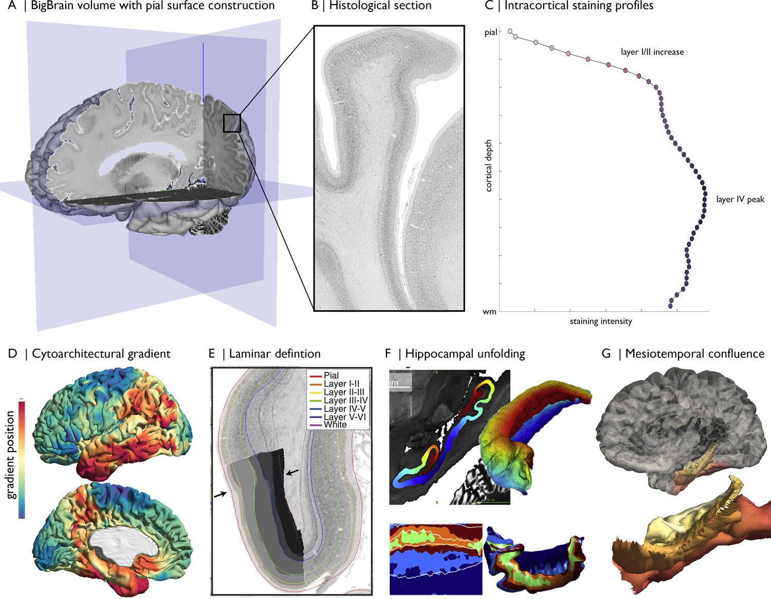
Magnification of cytoarchitecture using BigBrain, from (A) whole brain 3D reconstruction (taken on https://atlases.ebrains.eu/viewer) to (B) a histological section at 20 µm resolution (available from bigbrainproject.org) to (C) an intracortical staining profile.
The profile represents variations in cellular density and size across cortical depths. Distinctive features of laminar architecture are often observable i.e., a layer IV peak. Note, the presented profile was subjected to smoothing as described in the following section. BigBrainWarp also supports integration of previous research on BigBrain including (D–E) cytoarchitectural and (F–G) morphological models (DeKraker et al., 2019; Paquola et al., 2020a; Paquola et al., 2019; Wagstyl et al., 2020).
Figure 2
Evaluating BigBrain–MRI transformations.
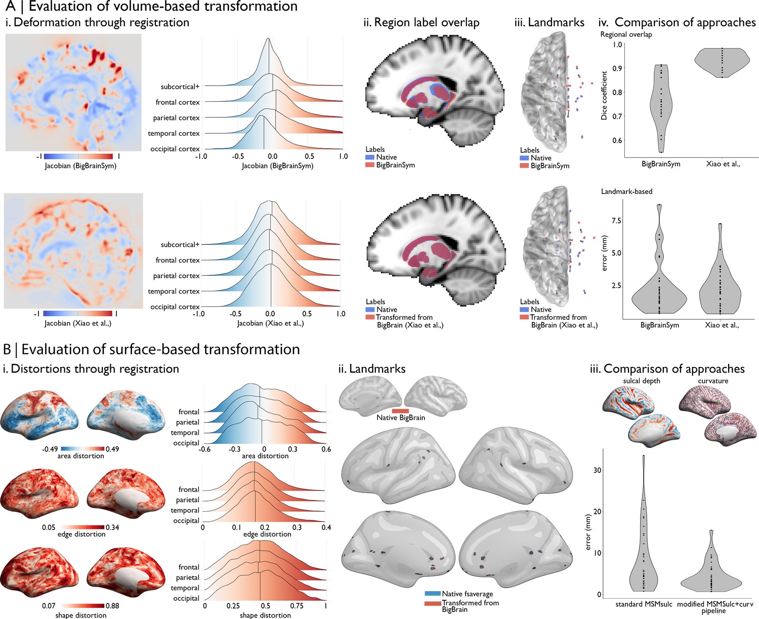
(A) Volume-based transformations. (i) Jacobian determinant of deformation field shown with a sagittal slice and stratified by lobe. Subcortical+ includes the shape priors (as described in Materials and methods) and the+ connotes hippocampus, which is allocortical. Lobe labels were defined based on assignment of CerebrA atlas labels (Manera et al., 2020) to each lobe. (ii) Sagittal slices illustrate the overlap of native ICBM2009b and transformed subcortical+ labels. (iii) Superior view of anatomical fiducials (Lau et al., 2019). (iv) Violin plots show the Dice coefficient of regional overlap (ii) and landmark misregistration (iii) for the BigBrainSym and Xiao et al., approaches. Higher Dice coefficients shown improved registration of subcortical+ regions with Xiao et al., while distributions of landmark misregistration indicate similar performance for alignment of anatomical fiducials. (B) Surface-based transformations. (i) Inflated BigBrain surface projections and ridgeplots illustrate regional variation in the distortions of the mesh invoked by the modified MSMsulc+ curv pipeline. (ii) Eighteen anatomical landmarks shown on the inflated BigBrain surface (above) and inflated fsaverage (below). BigBrain landmarks were transformed to fsaverage using the modified MSMsulc+ curv pipeline. Accuracy of the transformation was calculated on fsaverage as the geodesic distance between landmarks transformed from BigBrain and the native fsaverage landmarks. (iii) Sulcal depth and curvature maps are shown on inflated BigBrain surface. Violin plots show the improved accuracy of the transformation using the modified MSMsulc+ curv pipeline, compared to a standard MSMsulc approach.
Figure 3
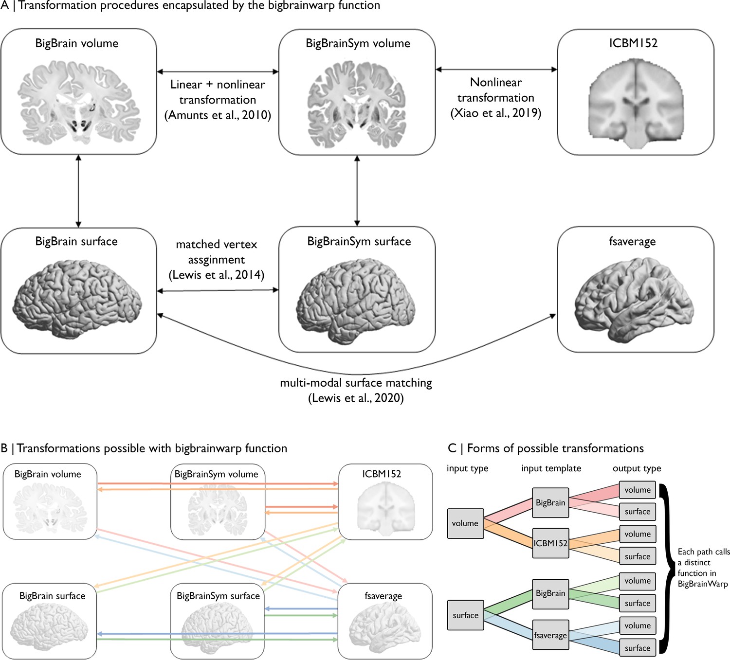
Overview of spaces and transformations included within BigBrainWarp.
(A) The flow chart illustrates the extant transformation procedures that are wrapped in by the bigbrainwarp function. (B) Arrows indicate the transformations possible using the bigbrainwarp function. The colours, matched to C, reflect distinct functions called within BigBrainWarp. (C) The combination of input type, input template, and output type determines the function called by BigBrainWarp.
Figure 4
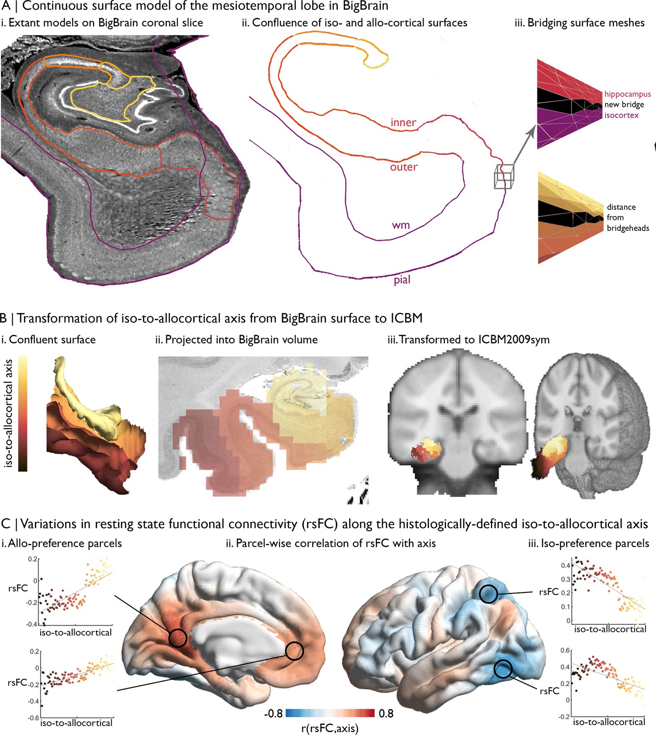
Intrinsic functional connectivity of the iso-to-allocortical axis of the mesiotemporal lobe.
(A) i. BigBrain surface models of the isocortex and hippocampal subfields are projected on a 40 µm resolution coronal slice of BigBrain. (ii–iii) The continuous surface model bridges the inner hippocampal vertices with pial mesiotemporal vertices (entorhinal, parahippocampal or fusiform cortex). Vertices at the medial aspect of the subiculum were identified as bridgeheads and used to bridge between the two surface constructions. Geodesic distance from the nearest bridgehead was used as the iso-to-allocortical axis. (B) Iso-to-allocortical axis values were projected from the surface into the BigBrain volume, then transformed to ICBM2009sym using BigBrainWarp. (C) Intrinsic functional connectivity was calculated between each voxel of the iso-to-allocortical axis and 1000 isocortical parcels. For each parcel, we calculated the product-moment correlation (r) of rsFC strength with iso-to-allocortical axis position. Thus, positive values (red) indicates that rsFC of that isocortical parcel with the mesiotemporal lobe increases along the iso-to-allocortex axis, whereas negative values (blue) indicate decrease in rsFC along the iso-to-allocortex axis.
Figure 5
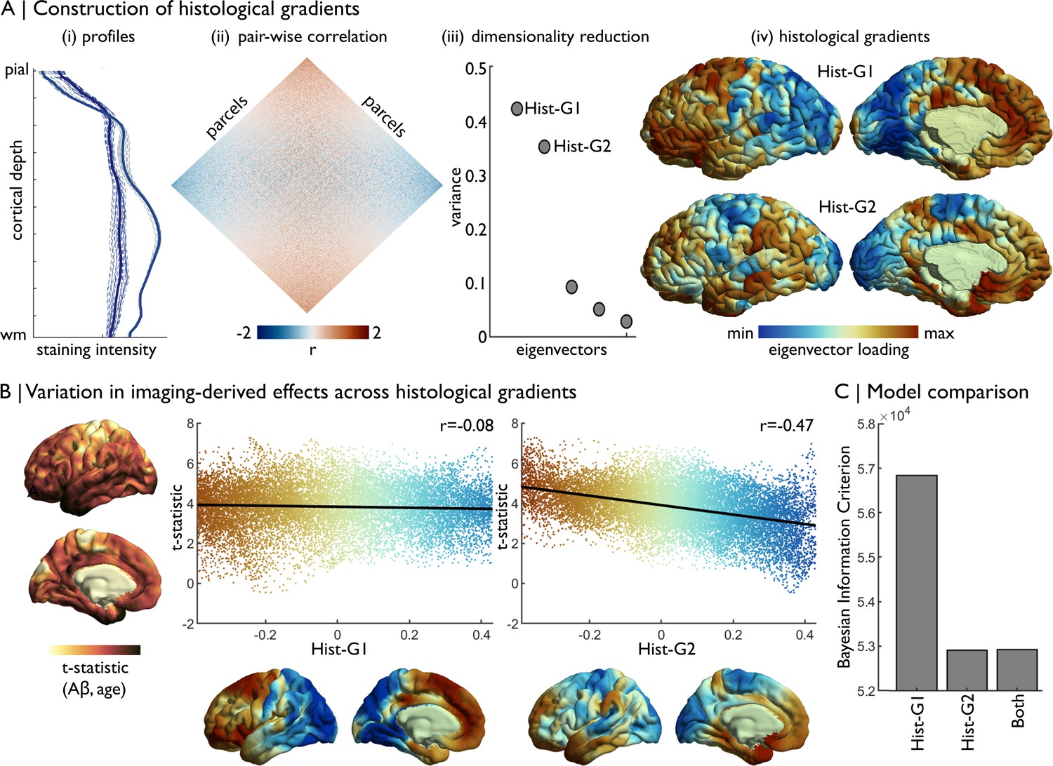
Concordance of imaging-derived effects with histological gradients.
(A) Four stages of histological gradient construction. (i) Vertex-wise staining intensity profiles (dotted lines) are averaged within parcels (solid lines). Colours represent different parcels. (ii) Pair-wise partial correlation of parcel-average staining intensity profiles produces a cortex-wide matrix of cytoarchitectural similarity. (iii) The correlation matrix is subjected to dimensionality reduction, in this case diffusion map embedding, to extract the eigenvectors of cytoarchitectural variation. (iv) The eigenvectors capture histological gradients (Hist-G) and are projected onto the BigBrain cortical surface for inspection. (B) The t-statistic cortical map illustrates regional variations in the effect of age on Aβ deposition (Lowe et al., 2019), which was calculated vertex-wise on fsaverage5. To allow comparison, histological gradients were transformed to fsaverage5 using BigBrainWarp. Scatterplots show the association of the t-statistic map with the histological gradients. (C) Bar plot shows the Bayesian Information Criterion of univariate and multivariate regression models, using histological gradients to prediction regional variation in effect of age on Aβ deposition. The univariate Hist-G2 regression had the lowest Bayesian Information Criterion, representing the optimal model of those tested.
Figure 6
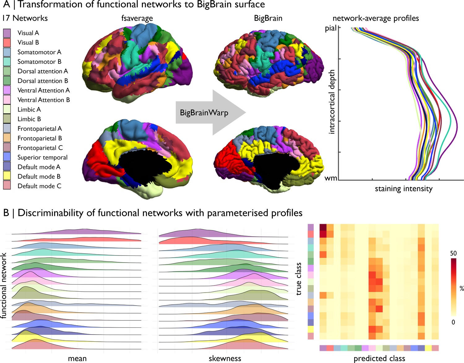
Prediction of functional network by cytoarchitecture.
(A) Surface-based transformation of 17-network functional atlas to the BigBrain surface, operationalised with BigBrainWarp, allows staining intensity profiles to be stratified by functional network. (B) Ridgeplots show the moment-based parameterisation of staining intensity profiles within each functional network. The confusion matrix illustrates the outcome of mutli-class classification of the functional networks, using the central moment of the staining intensity profiles.
Appendix 1—figure 1
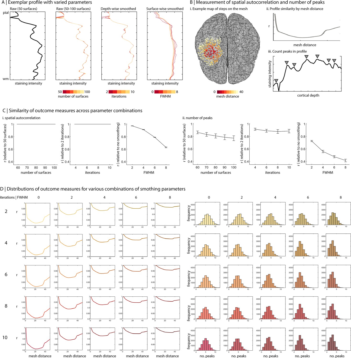
Influence of sampling parameters on staining intensity profiles.
(A) Line plots show how the shape of an exemplar profile is changed by various sampling parameters. Far left is the raw profile constructed with 50 surfaces. Centre left are raw profiles constructed with 50–100 surfaces. Centre right are profiles (constructed with 50 surfaces) and subjected to varied levels of depth-wise smoothing. Far right are profiles (constructed with 50 surfaces and subjected to 10 iterations of depthwise smoothing) with varied levels of surface-wise smoothing. (B) Influence of sampling parameters was evaluated based on spatial autocorrelation and number of peaks. (i–ii) The spatial autocorrelation was defined by the number of steps between two vertices on the mesh, as depicted for an example vertex in (i). Then, we calculated the product-moment correlation between all staining intensity profiles and averaged these values based on the relative distance between vertices. The line plot show a decrease in correlation with increasing distance, attributable to spatial autocorrelation. (iii) The number of peaks was calculated to assess the jaggedness the staining intensity profile. (C) Using the lowest iteration of a sampling parameter as a baseline, we 31 calculated the product-moment correlation of profile features (spatial autocorrelation or number of peaks) with increases in the sampling parameter. In other words, the graph shows the similarity of solutions to the baseline sampling parameters. We found that the surface-wise smoothing impacts the spatial autocorrelation and number of peaks, while the number of surfaces and depthwise smoothing have little-to-no effect on spatial autocorrelation and a small effect on number of peaks. (D) For varying degrees of depth-wise (rows) and surface-wise (columns) smoothing, line plots show spatial autocorrelation and histograms show the distribution of number of peaks across profiles.
Tables
Table 1
Surface constructions for BigBrain.
| Surfaces | Utility | Reference |
|---|---|---|
| Grey and white | Initialisation and visualisation | Lewis et al., 2014 |
| Layer 1/2 and layer 4 | Boundary conditions | Wagstyl et al., 2018a |
| Equivolumetric | Staining intensity profiles | Waehnert et al., 2014 |
| Deep learning laminar | Laminar thickness | Wagstyl et al., 2020 |
| Hippocampal | Initialisation and visualisation | DeKraker et al., 2019 |
| Mesiotemporal confluence | Initialisation and visualisation | Paquola et al., 2020a |
-
Note: Initialisation broadly refers to an input for feature generation, for example creation of staining intensity profiles or surface transformations.
Table 2
Input parameters for the bigbrainwarp function.
| Parameter | Description | Conditions | Options |
|---|---|---|---|
| in_space | Space of input data | Required | bigbrain, bigbrainsym, icbm, fsaverage, fs_LR |
| out_space | Space of output data | Required | bigbrain, bigbrainsym, icbm, fsaverage, fs_LR |
| wd | Path to working directory | Required | |
| desc | Prefix for output files | Required | |
| in_vol | Full path to input data, whole brain volume. | Requires either in_vol, or in_lh and in_rh | Permitted formats: mnc, nii or nii.gz |
| ih_lh | Full path to input data, left hemisphere surface | Permitted formats: label.gii, annot, shape.gii, curv or txt | |
| ih_rh | Full path to input data, right hemisphere surface | ||
| interp | Interpolation method | Required for in_vol. Optional for txt input. Not permitted for other surface inputs. | For in_vol, can be trilinear (default), tricubic, nearest or sinc.For txt, can be linear or nearest |
| out_type | Specifies whether output in surface or volume space | Optional function for bigbrain, bigbrainsym and icbm output. Defaults to the same type as the input. | surface, volume |
| out_res | Resolution of output volume | Optional where out_type is volume. Default is 1 | Value provided in mm |
| out_den | Density of output mesh | Optional where out_type is surface. Default is 164 | For fs_LR out_space, 164 or 32 |
-
Note: the options are subject to change as the toolbox is expanded. Updates will be posted on https://bigbrainwarp.readthedocs.io/en/latest/pages/updates.html.
Table 3
BigBrainWarp contents.
| Data | Definition | Original space | Transformed spaces |
|---|---|---|---|
| Profiles | Staining intensity profiles, sampled at each vertex and across 50 equivolumetric surfaces | BigBrain | fsaverage, fs_LR (164 k and 32 k) |
| White | Grey/white matter boundary | BigBrain, fsaverage, fs_LR | |
| Sphere | Spherical representation of surface mesh | BigBrain, fsaverage, fs_LR | |
| Confluence | Continuous surface that includes isocortex and allocortex (hippocampus) from Paquola et al., 2020a | BigBrain | |
| Histological gradients | First two eigenvectors of cytoarchitectural differentiation derived from BigBrain | BigBrain | fsaverage, fs_LR (164 k and 32 k), icbm |
| Microstructural gradients | First two eigenvector of microstructural differentiation derived from quantitative in-vivo T1 imaging | fsaverage | BigBrain, |
| Functional gradients | First three eigenvectors of functional differentiation derived from rs-fMRI | fsaverage | BigBrain |
| Seven functional networks | Seven functional networks from Yeo et al., 2011 | fsaverage | BigBrain |
| 17 Functional networks | 17 Functional networks from Yeo et al., 2011 | fsaverage | BigBrain, icbm |
| Layer thickness | Layer thicknesses estimated from Wagstyl et al., 2020 | BigBrain | fsaverage, fs_LR (164 k and 32 k) |
-
Note: Datasets Are Named According to BIDS and Align with Recommendations From TemplateFlow (Ciric et al., 2021).
Additional files
Download links
A two-part list of links to download the article, or parts of the article, in various formats.
Downloads (link to download the article as PDF)
Open citations (links to open the citations from this article in various online reference manager services)
Cite this article (links to download the citations from this article in formats compatible with various reference manager tools)
The BigBrainWarp toolbox for integration of BigBrain 3D histology with multimodal neuroimaging
eLife 10:e70119.
https://doi.org/10.7554/eLife.70119


