Recovering mixtures of fast-diffusing states from short single-particle trajectories
- Department of Molecular and Cell Biology, Li Ka Shing Center for Biomedical and Health Sciences, University of California, Berkeley, United States
- CIRM Center of Excellence, University of California, Berkeley, United States
- Howard Hughes Medical Institute, United States
Figures
Figure 1 with 1 supplement
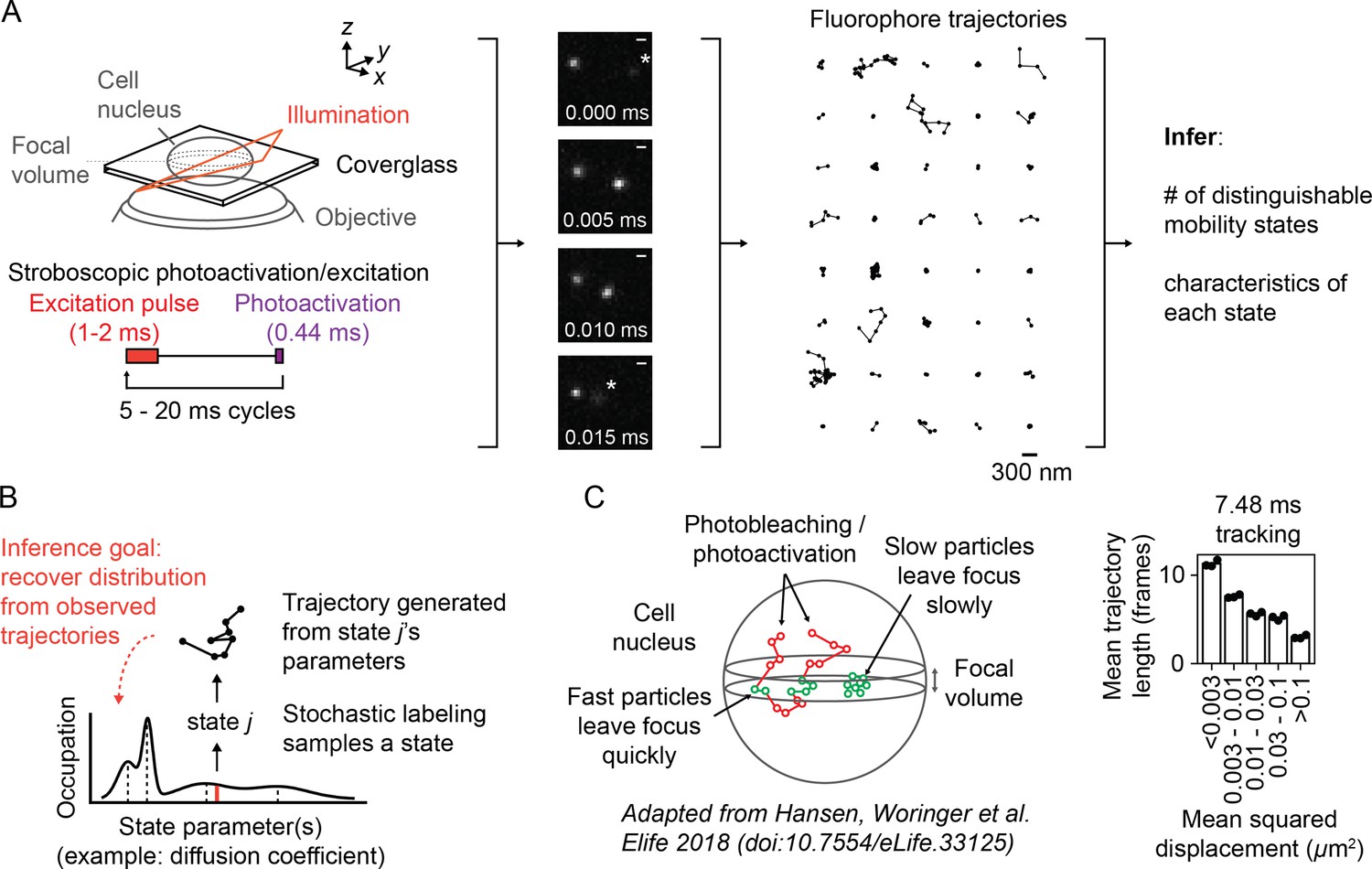
Overview of sptPALM.
(A) Schematic of experimental setup. An inclined illumination source is used in combination with a high-numerical aperture (NA) objective to resolve molecules in a thin slice in a cell. The excitation laser is pulsed to limit motion blur. Tracking yields a set of short trajectories (mean track length 3–5 frames). Trajectories shown are from a 7.48 ms tracking movie with retinoic acid receptor α-HaloTag (RARA-HaloTag) labeled with photoactivatable JF549 in U2OS nuclei. Asterisks in the movie frames mark particles at the edge of the focus. (B) Schematic of our inference problem. Each trajectory’s state is assumed to be a random draw from a distribution of state parameters. The goal is to recover this distribution from the observed trajectories. (C) Effects of particle mobility on trajectory length. RARA-HaloTag trajectories from U2OS nuclei were binned into five groups based on their mean squared displacement (MSD). Individual data points are the mean trajectory length of each group for three distinct knock-in clones of RARA-HaloTag (c156: 36961 trajectories, c239: 27543 trajectories, c258: 60347 trajectories); bar heights are the means across clones.
Figure 1—figure supplement 1
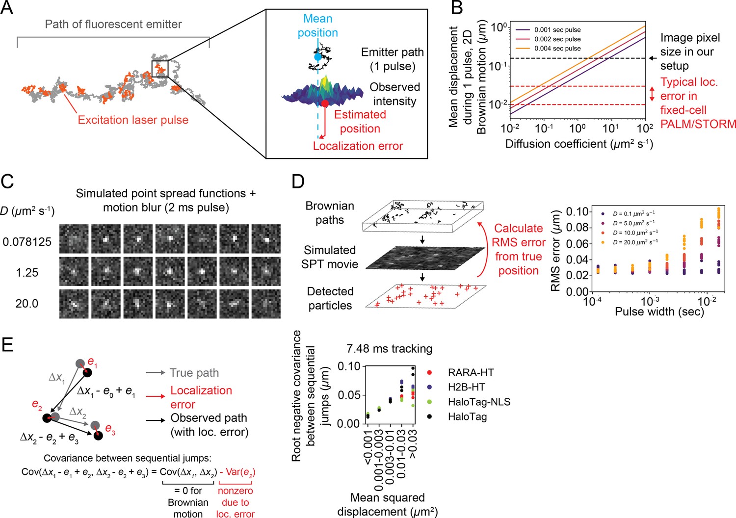
Demonstrations of the effect of motion blur on the sptPALM measurement.
(A) Illustration of motion blur. Because a fluorescent emitter has non-negligible movement during a single excitation pulse, the observed intensity distribution is not representative of a point source. Any pointwise estimate of its position, including those used in this article, incurs some error. (B) Mean displacement of a 2D Brownian motion during a single excitation pulse (). The black dotted line is the image pixel size used in the experiments in this manuscript (0.16 μm), while the red dotted line is a typical range of localization error for fixed cell PALM and STORM (10–30 nm). (C) Examples of simulated Brownian emitters with 2 ms excitation pulses. Imaging was simulated using the sptPALMsim package for a paraxial optical system (‘Materials and methods’). Also see Video 5. (D) Quantification of localization error for Brownian emitters simulated as in (C). Error was defined as the root mean squared deviation of the estimated position from the mean of the particle’s path during each pulse. (E) Scaling of estimated localization error with diffusion coefficient in real sptPALM. Trajectories were categorized according to their mean squared displacement (MSD) and for each category the localization error was estimated as the root negative covariance between sequential jumps. Individual data points in the graph represent biological replicates; each datapoint represents gt19000 trajectories on a separate coverslip in a separate biological clone (RARA-HT) or transfection (H2B-HT, HaloTag-NLS, HaloTag).
Figure 2 with 1 supplement
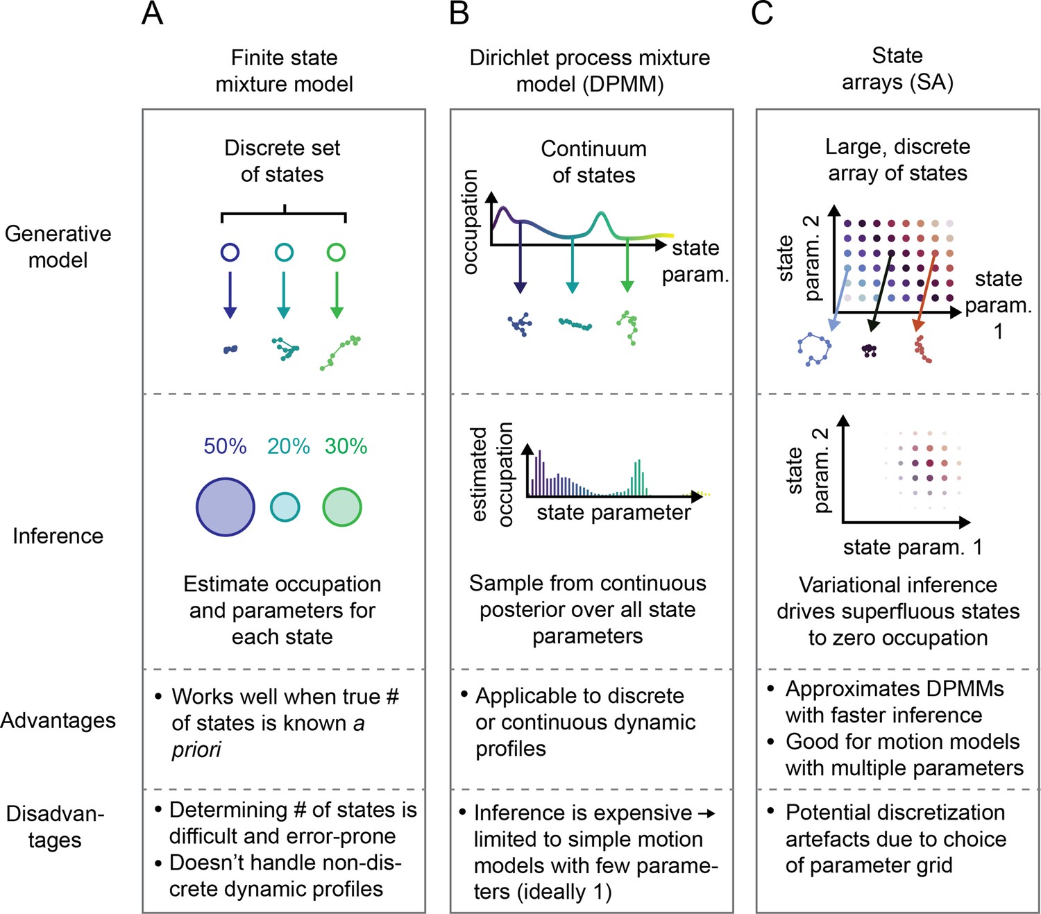
Schematic comparison of finite state mixtures, Dirichlet process mixtures, and state arrays (SAs).
(A) Finite state mixture models use a discrete set of states. Challenges include estimating and producing intelligible output when the underlying dynamic profile is not discrete. (B) Dirichlet process mixture models (DPMMs) address the problem of nondiscrete dynamic profiles by using a continuous distribution over state parameters. Inference routines are slow, so in this work we use approximative motion models. (C) SAs, a special case of the finite state mixture. SAs approximate DPMMs by using a discrete grid of state parameters and have a faster inference routine. Challenges with SAs include the choice of the parameter grid.
Figure 2—figure supplement 1
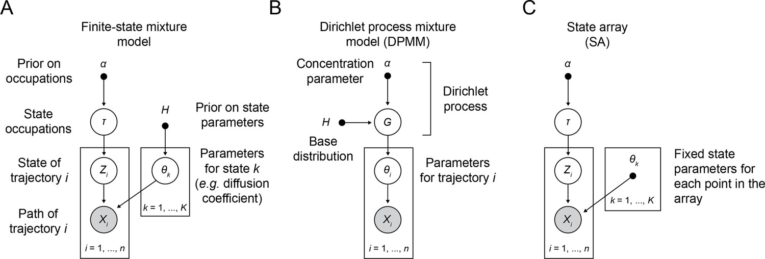
Probabilistic graphical models for finite state mixtures, Dirichlet process mixtures, and state arrays.
Open circles indicate random variables, shaded circles represented random variables that are observed in the sptPALM experiment, solid circles indicate constants, and arrows indicate conditional dependence (Bishop, 2006). (A) Graphical model for finite state mixtures. α is the concentration parameter for a Dirichlet prior over the state occupations. The usual goal is to infer the posterior . (B) Graphical model for Dirichlet process mixtures. α and are the parameters to a Dirichlet process used to generate candidate distributions . The usual goal is to infer the posterior . (C) Graphical model for state arrays. Notice that this is a special case of (A) when the state parameters are treated as constant. The goal is to infer .
Figure 3 with 2 supplements
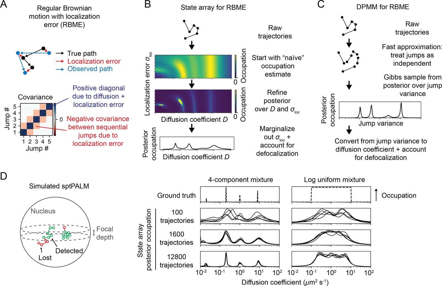
Application of state arrays and Dirichlet process mixture models (DPMMs) to mixtures of Brownian motions.
(A) Regular Brownian motion with localization error (RBME) is a motion model that involves two parameters: diffusion coefficient and localization error variance. (For brevity, we refer to the latter simply as ‘localization error.’) Unlike pure Brownian motion, RBME has correlations between sequential jumps due to the influence of localization error. (B) State array inference for RBMEs. The naive occupation estimate is the initial estimate for the posterior, which is subsequently refined through variational inference. At the end of inference, we marginalize out localization error to yield 1D distributions over the diffusion coefficient. (C) DPMM inference for mixtures of Brownian motions. Because the Gibbs sampling routine for a pure DPMM is slow, we use an approximative motion model that neglects the off-diagonal terms of the covariance matrix in (A). (D) Example of state arrays evaluated on simulated sptPALM. Tracking was simulated in a spherical nucleus with 700 nm focal depth, uniform photoactivation probability, 14 Hz bleaching rate, 7.48 ms frame intervals, and variable localization error. The lines represent the state array posterior mean occupations for independent replicates of the same simulation.
Figure 3—figure supplement 1
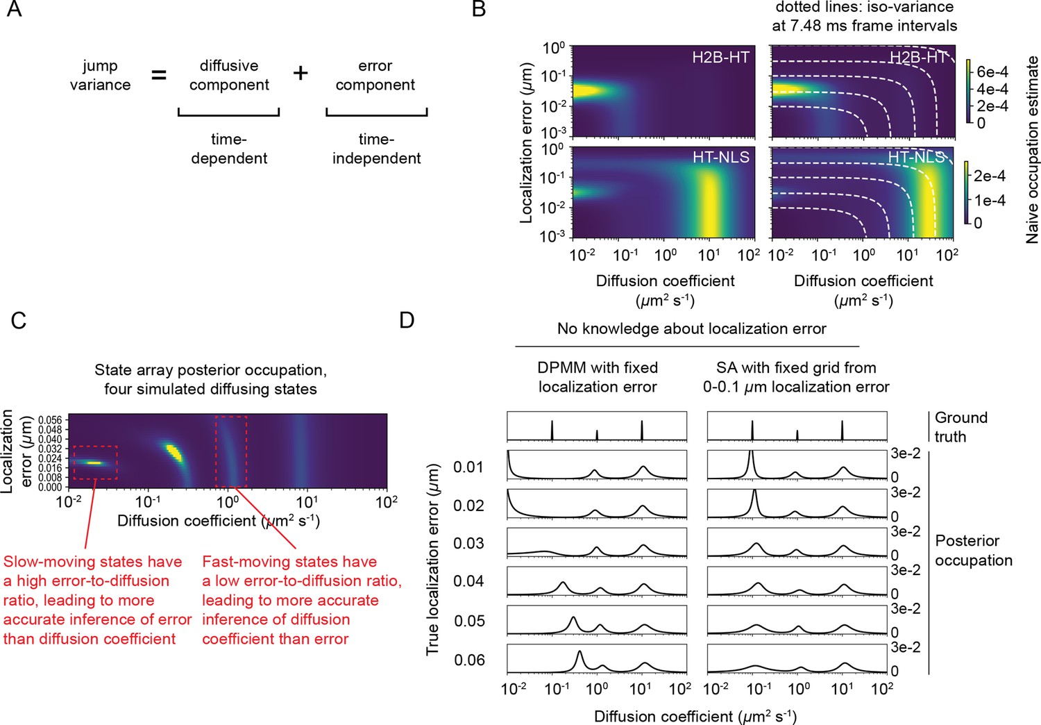
Challenges distinguishing between diffusion and localization error.
(A) The variance of the jumps of a regular Brownian motion with localization error (RBME) depends on both real diffusion and localization error. (B) Naive state occupation estimates for two experimental sptPALM datasets. Dotted white lines indicate contours in the state space with constant jump variance. (C) Illustration of the difficulty in coinference of diffusion coefficient and localization error for a simulated sptPALM dataset with four states. (D) Illustration of the danger of misestimating the localization error for the Dirichlet process mixture model (DPMM) method with simulated mixtures of three RBME states. In this case, the assumed localization error in the DPMM algorithm was held constant at 30 nm. Because state arrays (SAs) naturally incorporate uncertainty about localization error, inference is more stable with respect to changes in the experimental localization error. Note that this has a stronger effect on slower-moving states.
Figure 3—figure supplement 2
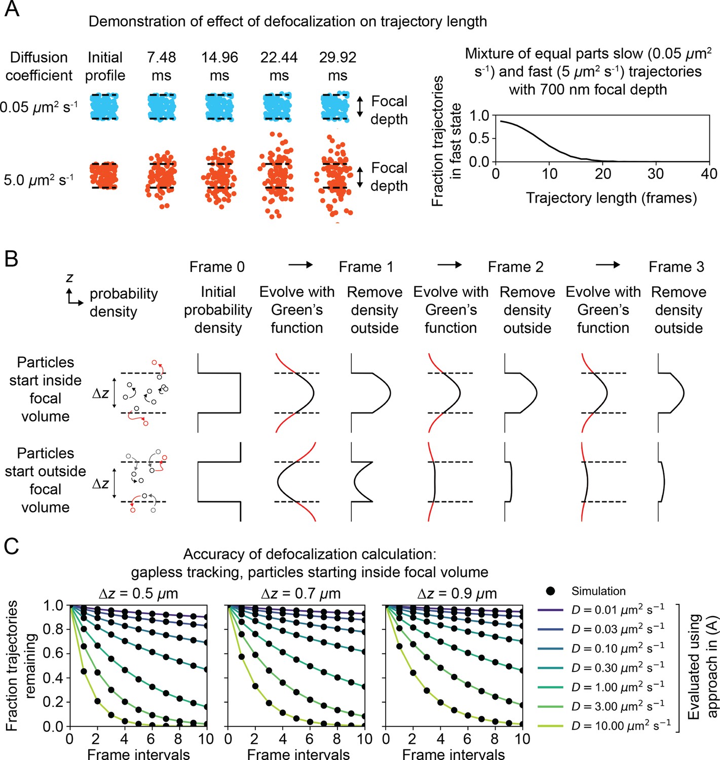
Accounting for the influence of defocalization on state occupations.
(A) Demonstration of the effect of defocalization on trajectory length. 340,727 Brownian trajectories were simulated in a 5 μm radius nucleus with a 700 nm focal depth and 14 Hz bleaching rate. The diffusion coefficients for each trajectory were drawn with equal probability from a slow state (0.05 μm2 s-1) and a fast state (5 μm2 s-1). Tracking was simulated without gaps, so that particles outside the focal volume at any frame interval are considered ‘lost’ for all subsequent frames. For each observed trajectory length, we quantified the fraction of trajectories with that length in the fast state. (B) Approach used to calculate the fraction of defocalized trajectories. Two possible initial probability densities for the particle in are shown. The Green’s function for the diffusion model is used to propagate the probability density. At each frame interval, the density that lies outside the focal volume (corresponding to particles that are not observed) is set to zero. (C) Comparison of the algorithm in (B) with the defocalized fraction from simulated data. Trajectories were initialized in a slab with thickness and infinite XY extent, then tracked without gaps. The fraction of trajectories remaining was quantified at each frame interval. Each black dot corresponds to a simulation with 100,000 trajectories, while the lines correspond to the output of the algorithm in (B).
Figure 4 with 12 supplements

Comparison of the mean squared displacement (MSD) histogram, Dirichlet process mixture model (DPMM), and state array (SA) methods to recover dynamic profiles from trajectory simulations.
(A–C) Mixtures of diffusing states were simulated in a 700 nm focal volume with 7.48 ms frame intervals. Simulations were divided into three classes of increasing difficulty based on the treatment of localization error as described in the text. For each replicate, exactly 12,800 trajectories were simulated. Estimated occupations for five independent replicates are overlaid on each subplot. (D) Accuracy of state occupation estimates for each method as a function of sample size. Each method was run on trajectory simulations generated from an underlying three-state dynamic model (0.02 μm2 s-1 [20%], 0.5 μm2 s-1 [30%], 5.0 μm2 s-1 [50%]), then occupations were estimated by integrating the distribution produced by each method. Limits of integration were set to 0–0.08 μm2 s-1 (state 1), 0.08–1.5 μm2 s-1 (state 2), or 1.5–40 μm2 s-1 (state 3). 20 replicates were run per condition. (E) Mean absolute error (MAE) in state occupation estimates for the simulations in (D). Each value is the average MAE across all replicates. (F) Inferring mixtures of diffusing states with similar diffusion coefficients using SAs. For each replicate, a total of 6400 trajectories were simulated with the indicated underlying state distribution. (G) Effect of state transitions on the MSD, DPMM, and SA approaches. We varied the first-order transition rate constant between two diffusing states, simulating 6400 trajectories per replicate.
Figure 4—figure supplement 1
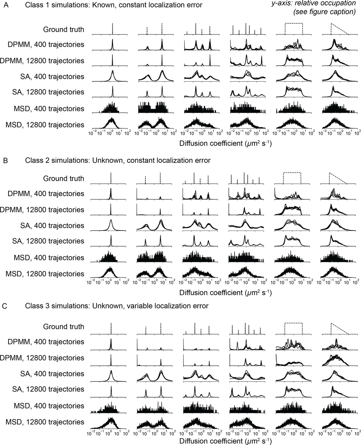
Comparison of Dirichlet process mixture models (DPMMs), state arrays (SAs), and mean squared displacement (MSD) histograms to estimate state occupations for several kinds of trajectory simulation.
In all panels, the y-axis represents the probability (or inferred probability) of a particular diffusion coefficient. In detail: for the ground truth, the y-axis is the probability of simulating a particular diffusion coefficient. For the MSD approach, the y-axis is the proportion of trajectories with estimated diffusion coefficients that fall into the corresponding bin. For the DPMM and SA methods, the y-axis is the posterior probability of each of a discrete set of diffusion coefficient bins spanning 0.01–100.0 μm2 s-1. In the case of SA, this posterior probability has been marginalized over the localization error component. Five independent replicates are overlaid on each subplot. (A) ‘Class 1’ simulations with known and constant localization error (standard deviation 30 nm). (B) ‘Class 2’ simulations with constant but unknown localization error (standard deviation 30 nm). In the cases of DPMM and MSD, the localization error was first inferred using jump covariance and then held constant when estimating the distribution over the diffusion coefficient. In the case of SA, the localization error is jointly inferred with the diffusion coefficient. (C) ‘Class 3’ simulations with variable and unknown localization error. Inference proceeded as in (B), but in the case of the MSD approach, the localization error and diffusion coefficient were jointly inferred for each trajectory.
Figure 4—figure supplement 2

Quantitative comparison of the results in Figure 4—figure supplement 1.
Accuracy of the mean squared displacement (MSD) histogram, Dirichlet process mixture model (DPMM), and state array (SA) methods for estimating dynamic profiles. The trajectory simulations were the same as in Figure 4—figure supplement 1 using 12,800 simulated trajectories. (A) In order to compare the simulated ground truth profile (which could be discrete or continuous) with the output of each method, we quantified the root mean squared deviation (RMSD) of the estimated cumulative distribution function (CDF) from the ground truth CDF. (B) Accuracies of each method in terms of CDF RMSD. Each value is the average CDF RMSD over five replicates. (C) Scatterplot of CDF RMSDs for each simulation replicate in (B). Each dot represents a replicate of the same simulation.
Figure 4—figure supplement 3
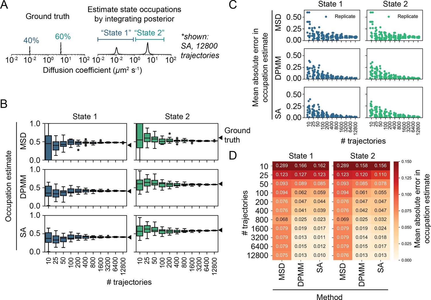
Effect of sample size on accuracy and precision of the mean squared displacement (MSD) histogram, Dirichlet process mixture model (DPMM), and state array (SA) methods using two-state trajectory simulations.
(A) Trajectories were simulated with two distinct diffusion coefficients (0.1 μm2 s-1 [40% occupation] and 5.0 μm2 s-1 [60% occupation]) in a 5 μm sphere with specular reflections, 7.48 ms frame intervals, 14 Hz bleaching rate, and a 700 nm focal depth (‘Materials and methods’). Occupation estimates were derived by integrating the normalized histogram (for the MSD method) or the mean of the posterior distribution (for DPMM and SA methods). The limits of integration for each state were identical for all methods: 0–1 μm2 s-1 (state 1) and 1–40 μm2 s-1 (state 2). (B) Estimated occupations for each state according to each method (20 replicates per sample size). (C) Mean absolute error (MAE) of state occupation estimates for each replicate in (B). (D) Tabular presentation of the data in (C). Each number is the MAE averaged across all replicates for that simulation.
Figure 4—figure supplement 4
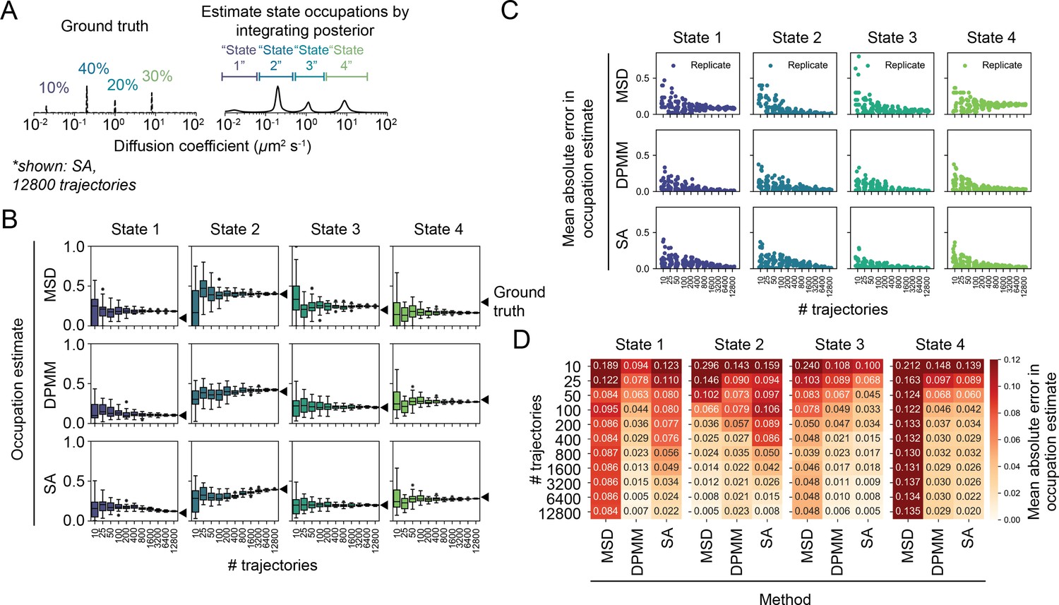
Effect of sample size on accuracy and precision of the mean squared displacement (MSD) histogram, Dirichlet process mixture model (DPMM), and state array (SA) methods using four-state trajectory simulations.
(A) Trajectories were simulated with four distinct diffusion coefficients: 0.02 μm2 s-1 (10% occupation), 0.2 μm2 s-1 (40% occupation), 1.0 μm2 s-1 (20% occupation), or 8.0 μm2 s-1 (30% occupation). Apart from the dynamic model, the simulation was performed as in Figure 4—figure supplement 3. Occupation estimates were derived by integrating the normalized histogram (for the MSD method) or the mean of the posterior distribution (for DPMM and SA methods). The limits of integration for each state were identical for all methods: 0.0–0.08 μm2 s-1 (state 1), 0.08–0.5 μm2 s-1 (state 2), 0.5–3 μm2 s-1 (state 3), and 3–40 μm2 s-1 (state 4). (B) Estimated occupations for each state according to each method (20 replicates per sample size). (C) Mean absolute error of state occupation estimates for each replicate in (B). (D) Tabular presentation of the data in (C). Each number is the average across all replicates for that simulation.
Figure 4—figure supplement 5
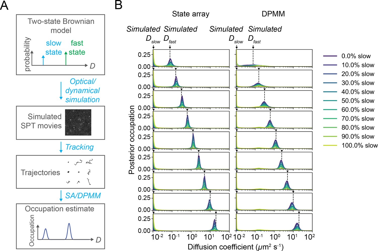
State array and Dirichlet process mixture model (DPMM) performance on optical–dynamical simulations of sptPALM movies with two diffusing states.
(A) Summary of approach. We simulated a paraxial imaging system and generated SPT movies by systematically varying the state occupations and fast diffusion coefficients for a two-state Brownian model (‘Materials and methods’). After simulation, we ran tracking and state array or DPMM inference, then compared the recovered state occupations with the simulated ground truth. About 5000 trajectories were identified by the tracking algorithm per condition. (B) Posterior mean occupations for each simulated condition. Each row corresponds to a distinct value for and each color to a distinct slow state occupation; arrows indicate the simulated ground truth states.
Figure 4—figure supplement 6
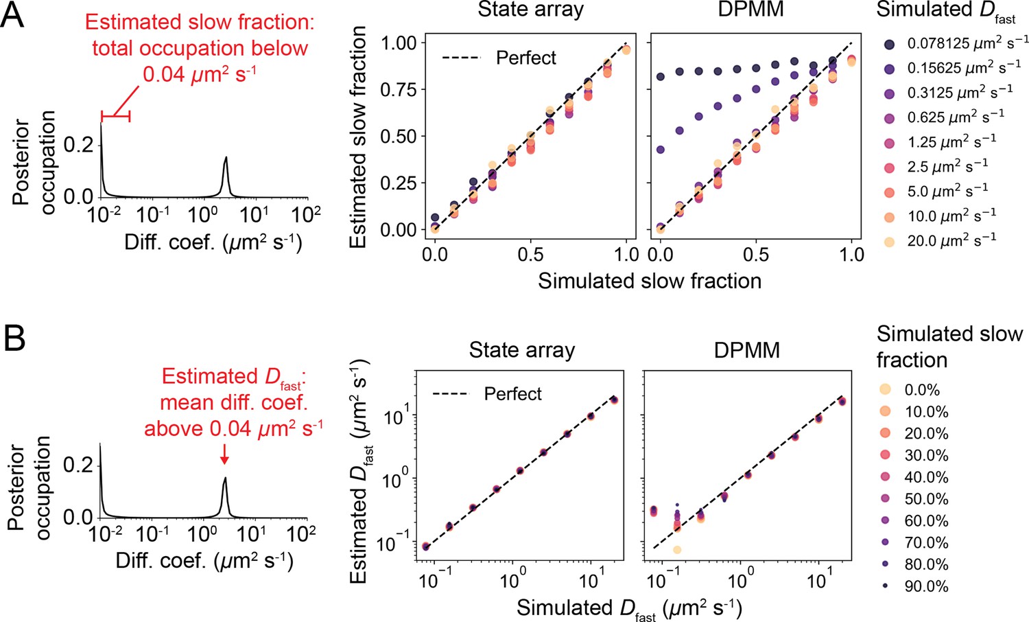
State array and Dirichlet process mixture model (DPMM) accuracy 2.
Quantitative evaluation of state array and DPMM performance on optical–dynamical simulations from Figure 4—figure supplement 5. (A) Accuracy of state occupation retrieval. The ‘slow fraction’ was defined as the integrated posterior occupation below 0.04 μm2 s-1 and compared against the ground truth. (B) Accuracy of fast diffusion coefficient estimation. The fast diffusion coefficient (‘’) was defined as the mean diffusion coefficient above 0.04 μm2 s-1.
Figure 4—figure supplement 7

Effect of state transitions on Dirichlet process mixture model (DPMM) and state array (SA) methods.
(A) State diagram for two-state regular Brownian motion with first-order state transitions. The transition rate constant was identical for both transitions. (B) Settings for the state transition simulations. Under these conditions, the mean trajectory length was 7 frames. 6400 trajectories were used for each run. (C) Outcome of the simulations. The y-axis corresponds to the occupation or occupation estimate for a particular diffusion coefficient. Specifically, for the ground truth column, the y-axis is the probability to simulate a particular diffusion coefficient; for mean squared displacement (MSD), it is the fraction of trajectories with estimated diffusion coefficients that fall into the respective bin; for the DPMM and SA methods, it is the posterior mean occupation estimate. For both DPMMs and SAs, we used a maximum trajectory length of 12 frames. For the MSD, DPMM, and SA methods, the result of inference with five independent replicates is overlaid on each subplot.
Figure 4—figure supplement 8
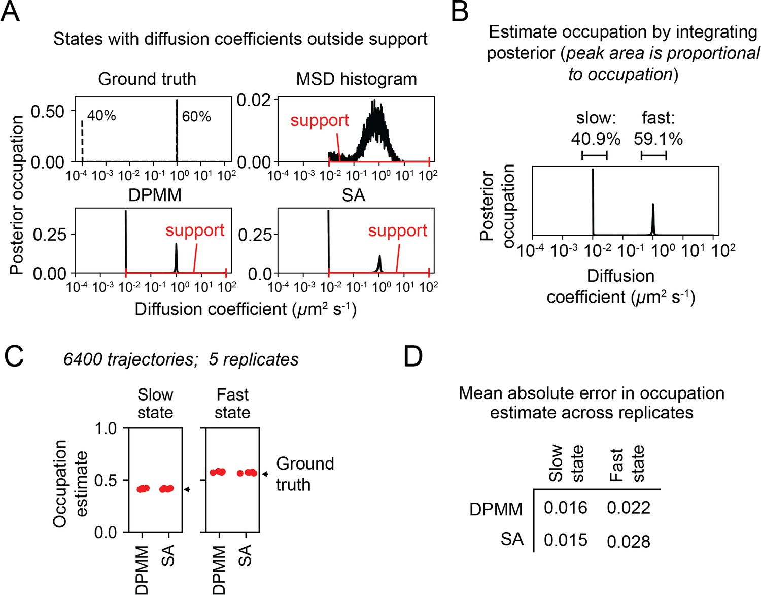
Performance of Dirichlet process mixture model (DPMM) and state array (SA) methods on states with diffusion coefficients slower than the minimum diffusion coefficient included in the support.
(A) Schematic of approach. We performed a trajectory simulation with two states, including one with a diffusion coefficient (10-4 μm2 s-1) smaller than the smallest supported diffusion coefficient for the three methods (10-2 μm2 s-1). Five replicates are overlaid on each subplot. (B) State occupations were estimated by integrating the posterior mean over the peaks. Note that a peak appears at 10-2 rather than the simulated 10-4. (C) Estimates for the occupation of the slow and fast states with each method. (D) Mean absolute error of the state occupation estimates in (C). The value reported is the mean of the mean absolute error over the five replicates.
Figure 4—figure supplement 9
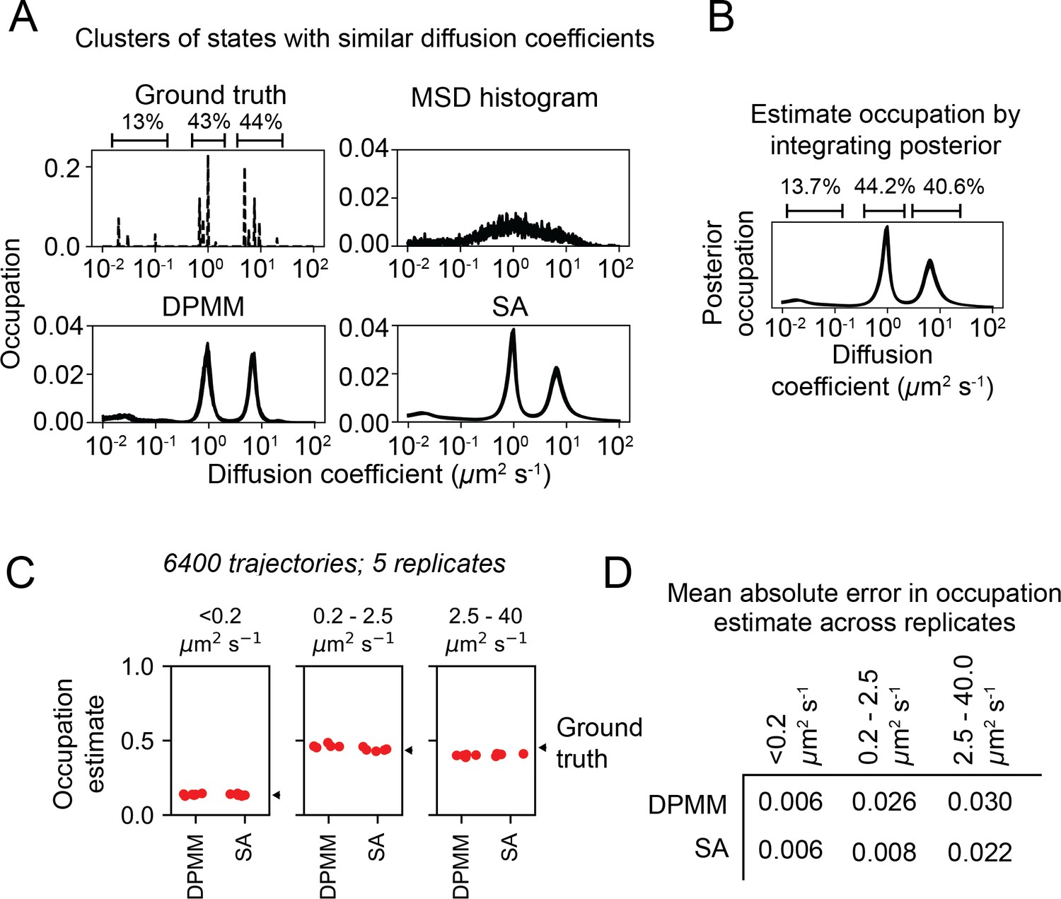
Performance of Dirichlet process mixture model (DPMM) and state array (SA) algorithms on clusters of states with similar diffusion coefficients.
(A) Schematic of approach. We performed a trajectory simulation with three clusters of states with similar diffusion coefficients, then analyzed these simulations with the mean squared displacement (MSD) histogram, DPMM, or SA methods. Five replicates are overlaid on each subplot. Notice that none of the three methods could distinguish the states within each cluster. (B) Occupation estimates for each of the three clusters were estimated by integrating the posterior mean over the following ranges: 0–0.2 μm2 s-1, 0.2–2.5 μm2 s-1, and 2.5–40 μm2 s-1. (C) Estimates for the occupation of each cluster of states. (D) Mean absolute error of the state occupation estimates in (C). The value reported is the mean of the mean absolute error over the five replicates.
Figure 4—figure supplement 10
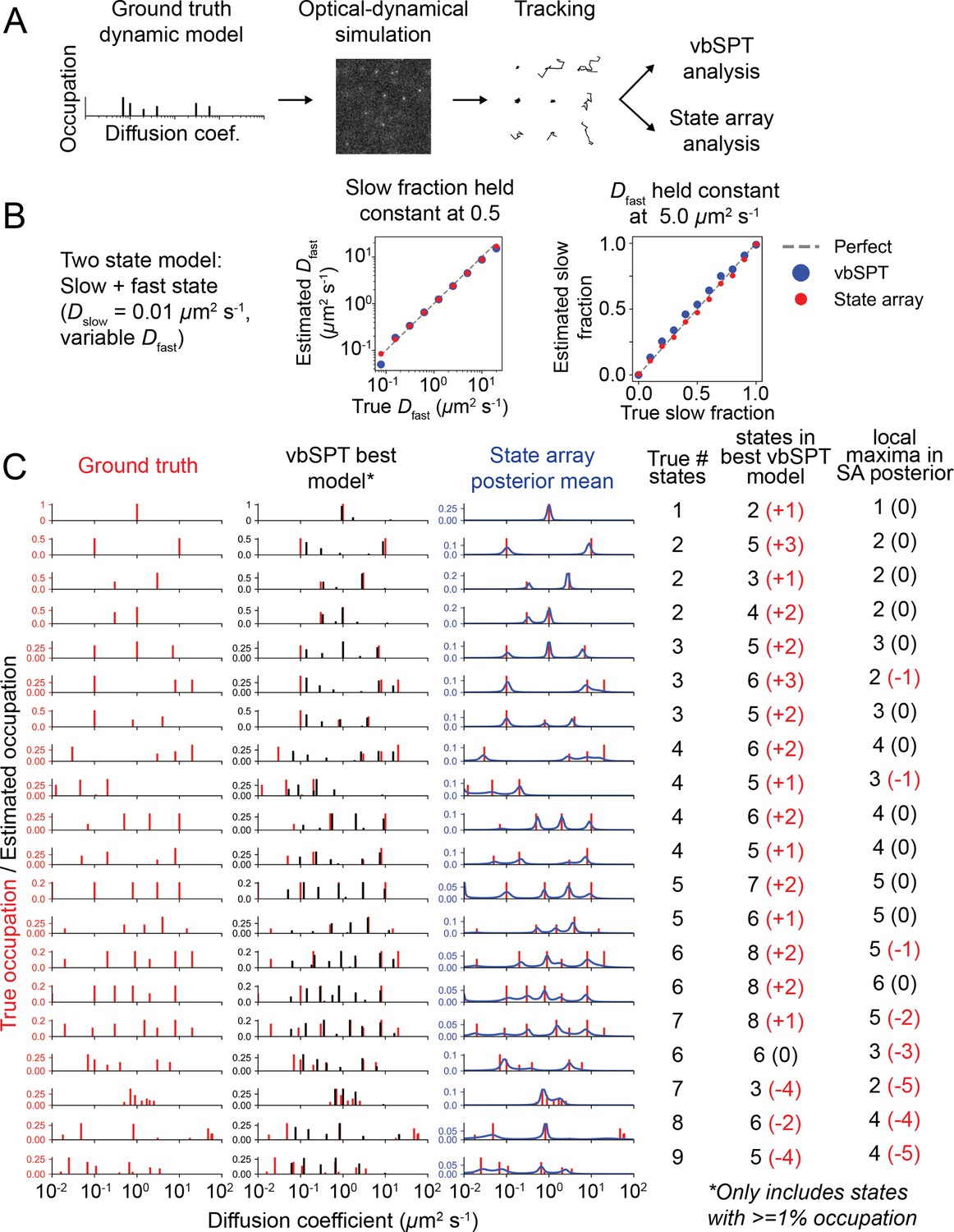
Comparison of state arrays with vbSPT with optical–dynamical simulations.
(A) Schematic of approach. sptPALM movies were simulated with an underlying multistate Brownian motion model. These were tracked and analyzed with state arrays and vbSPT. We do not consider the ability of vbSPT to estimate transition rates, and no state transitions were included in the simulation. (B) Comparison of vbSPT and state array accuracy on models with two states. Because the number of states returned by vbSPT is variable (between 2 and 7 for this data), we estimated as the state closest to the true . For state arrays, was estimated as the mode of the posterior distribution above 0.02 μm2 s-1. For both methods, the slow fraction was estimated as the sum of the occupation of all states below 1.0 μm2 s-1. (C) Comparison of vbSPT and state arrays on various dynamic models. Each row corresponds to a particular dynamic model, as shown in the left column. The -axis corresponds to true occupation for the ‘Ground truth’ column, occupation of the best model for vbSPT, and the mean posterior occupation for state arrays. On average, 5510 trajectories were tracked in each simulation. In the table at the right, the numbers in parentheses are the deviation from the true number of simulated states.
Figure 4—figure supplement 11
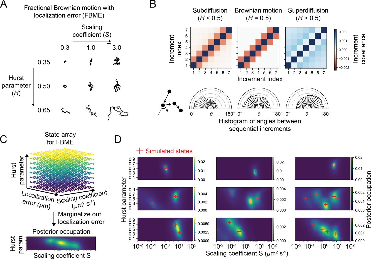
State arrays applied to fractional Brownian motion with localization error (FBME) using optical–dynamical simulations.
(A) Example FBME trajectories. The two parameters of interest are the modified scaling coefficient (parameterizing the size of the increments, analogous to the diffusion coefficient) and the Hurst parameter (parameterizing correlations between increments). (B) Increment covariance matrices and angular distributions for the three main regimes of FBME. Notice that the localization error term contributes to the off-diagonal terms in the covariance, resulting in a departure from pure FBM. (C) Schematic of state array for FBME. The state array is comprised of a 3D parameter array of , , and localization error variance. After inference, the posterior is marginalized over localization error to yield 2D functions of and . (D) Posterior occupation for various simulated multistate FBM models. SPT movies were simulated with the sptPALMsim package (‘Materials and methods’); red crosshairs indicate the ground truth simulated states.
Figure 4—figure supplement 12
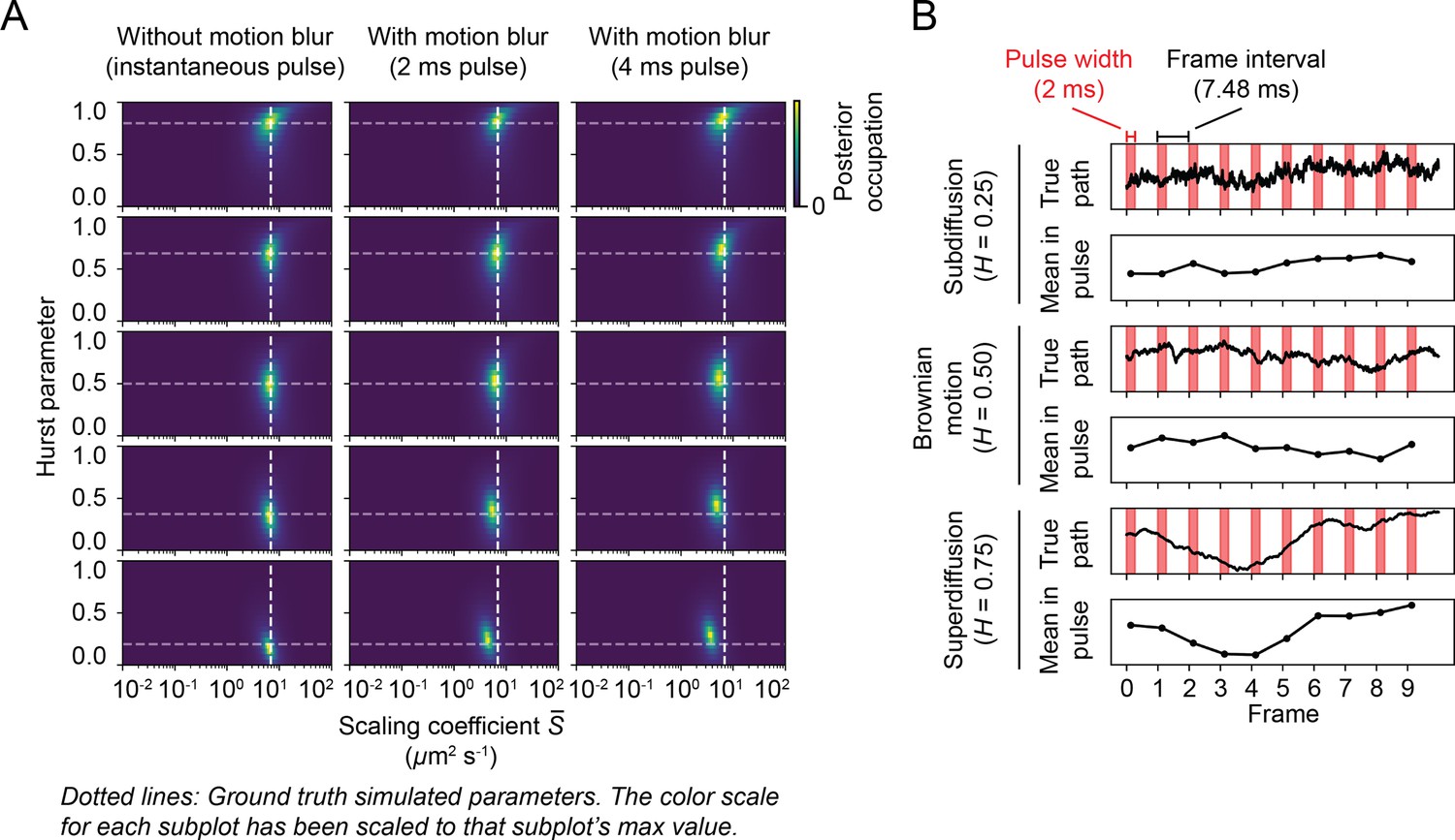
Systematic errors in fractional Brownian motion with localization error (FBME) parameter retrieval due to motion blur.
(A) State array posterior distributions for single-state FBME models, simulated as in Figure 4—figure supplement 11. Each subplot represents the posterior distribution for simulations of one motion model. The ground truth model’s Hurst parameter is indicated with a horizontal gray dotted line and the scaling coefficient with a vertical white dotted line. (B) Rationalization of the effect in panel (A). The ‘true path’ is a simulated FBM, the red bars indicate the simulated excitation laser pulses, and ‘mean in pulse’ is the mean position of each particle during each excitation laser pulse. Motion blur may exert a more significant effect for low Hurst parameters because the corresponding FBMEs have more motion in the higher temporal frequencies, which is averaged out over each pulse.
Figure 5 with 2 supplements
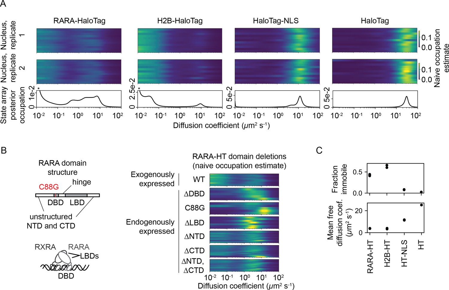
State arrays (SAs) applied to experimental sptPALM.
All sptPALM experiments were performed with the photoactivatable dye PA-JFX549 using a TIRF microscope with HiLo illumination, 7.48 ms frame intervals, and 1 ms excitation pulses. (A) Naive and SA occupations for four different tracking targets. The upper two panels are the naive occupations for each nucleus in each of two biological replicates. Biological replicates correspond to separate knock-in clones for RARA-HaloTag or separate transfections for the other constructs (mean 1627 trajectories per nucleus). The bottom panel displays the SA occupations for a run of the SA algorithm on trajectories pooled from a single biological replicate (mean 17,899 trajectories per biological replicate). Asterisks for RARA-HaloTag and H2B-HaloTag indicate that the immobile fraction for these constructs has been truncated to visualize the faster-moving states. (B) Naive occupation estimate for RARA-HaloTag constructs bearing domain deletions or point mutations. ‘Exogenously expressed’ constructs were expressed from a nucleofected PiggyBac vector under an L30 promoter. (C) Quantification of the immobile fractions and mean free diffusion coefficients for the four constructs in (A). The ‘immobile fraction’ was defined as the total occupation below 0.05 μm2 s-1, while the mean free diffusion coefficient was the posterior mean diffusion coefficient above this threshold. Each dot represents a biological replicate (a different knock-in clone for RARA-HT or a different nucleofection for H2B-HT, HT-NLS, and HT).
-
Figure 5—source data 1
Raw and labeled RARA-HaloTag Western blots used in Figure 5.
- https://cdn.elifesciences.org/articles/70169/elife-70169-fig5-data1-v2.zip
Figure 5—figure supplement 1

Validation of endogenously tagged U2OS RARA-HaloTag cell lines.
In all subpanels, ‘atRA’ refers to all-trans retinoic acid. (A) Western blots for endogenous RARA-HaloTag knock-ins in U2OS cells. The expected molecular weight of RARA-HaloTag-3xFLAG is 97 kDa. (B) Luciferase assays with a retinoic acid-responsive promoter with wildtype or RARA-HaloTag knock-in U2OS cell lines. (C) Luciferase assays with transfected RARA constructs to assess the effect of tagging on transactivation of a retinoic acid response element-driven luciferase gene. RARA(WT) indicates a transgene bearing the wildtype version of RARA, and C88G is a DNA-binding mutant. (D) Spinning disk confocal microscopy images of endogenously tagged RARA-HaloTag cell lines labeled with TMR-HaloTag ligand. The intensities for all three images have been scaled to the same min/max in arbitrary intensity units.
Figure 5—figure supplement 2
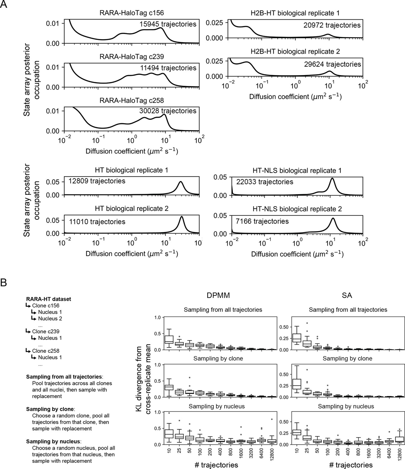
Assessing variability of state arrays (SAs) on experimental sptPALM by subsampling.
(A) Biological replicates of each of the tracking experiments shown in Figure 5A. Tracking was performed on an inverted TIRF setup with 7.48 ms frame intervals and 1 ms stroboscopic excitation with the dye PAJFX549-HaloTag ligand. RARA-HT cells were knock-ins as described in Figure 5—figure supplement 1, H2B-HaloTag cells were previously described (McSwiggen et al., 2019), and HT and HT-NLS were expressed from a nucleofected PiggyBac vector under an EF1α promoter. (B) Resampling experiment to evaluate the sources of variability in DPMM/SA runs on RARA-HaloTag trajectories. RARA-HaloTag trajectories from one tracking dataset were sampled according to one of three schemes, then analyzed with the Dirichlet process mixture model (DPMM) and SA methods. 20 replicates were performed for each condition, and the Kullback–Leibler divergence of the posterior occupation of each replicate from the cross-replicate posterior occupation was used to quantify variability.
Figure 6 with 1 supplement

Spatiotemporal variation in the state array posterior distribution.
(A) Posterior occupations for a state array evaluated on NPM1-HaloTag trajectories in U2OS nuclei. The ranges labeled i, ii, iii, and iv indicate parts of the dynamic profile isolated for analysis in subsequent panels. (B) Spatial distribution of the posterior probability in (A) for NPM1-HaloTag trajectories in a single U2OS nucleus. The posterior model over the diffusion coefficient was evaluated for each of the origin trajectories, and these points were then used to perform a kernel density estimate (KDE) with a 100 nm Gaussian kernel. For the local normalized occupation, these KDEs were normalized to estimate the relative fractions of molecules in each state. (C) Quantification of the analysis in (B) for 15 nuclei. ‘Nucleoplasmic’ trajectories were defined as trajectories outside nucleoli but inside the nucleus. (D) Temporal variation in the posterior distribution.
Figure 6—figure supplement 1
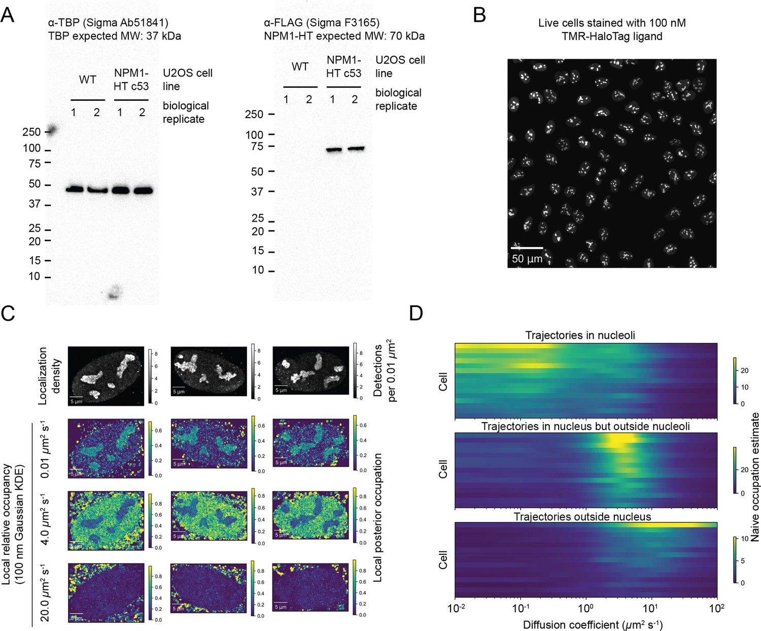
Validation of U2OS NPM1-HaloTag lines.
(A) Western blots of heterozygously tagged NPM1-HaloTag-3xFLAG in U2OS nuclei. (B) U2OS NPM1-HaloTag cells stained with 100 nM TMR-HaloTag ligand and imaged on a spinning disk confocal microscope. (C) Additional examples of cells quantified as in Figure 6B. The local occupation estimate is the fraction of particles in each neighborhood estimated to have the corresponding range of diffusion coefficients, as indicated in Figure 6B. To aid visualization, both localization density and local occupations were smoothed via convolution with a 2D isotropic Gaussian kernel of sigma 100 nm. (D) Naive occupation estimate for trajectories in different subcellular compartments. Trajectories were classified as either inside nucleoli, ‘nucleoplasmic’ (outside nucleoli but inside the nucleus), or extranuclear. The regular Brownian motion with localization error (RBME) likelihood function was evaluated on each set of trajectories, aggregated across trajectories and plotted as a function of the diffusion coefficient. Each row in the plot is separate nucleus, and the occupation estimates have been scaled for each compartment by the total number of trajectories.
-
Figure 6—figure supplement 1—source data 1
Raw and labeled NPM1-HaloTag Western blots.
- https://cdn.elifesciences.org/articles/70169/elife-70169-fig6-figsupp1-data1-v2.zip
Videos
Video 1
Example of sptPALM data.
NPM1-HaloTag in U2OS osteosarcoma nuclei was labeled with 100 nM PA-JFX549-HTL for 5 min followed by washes (‘Materials and methods’), then imaged with a HiLo setup at 7.48 ms frame intervals with 1.5 ms excitation pulses. The pixel size after accounting for magnification is 160 nm. Dots and lines indicate the output of the detection and tracking algorithm; each trajectory has been given a distinct color.
Video 2
Illustration of defocalization for a single regular Brownian state.
Trajectories were simulated in a 5 × 5 × 10 μm ellipsoid μm using the Euler–Maruyama scheme for regular Brownian motions with specular reflections at the ellipsoid boundaries. The diffusion coefficient for all trajectories was held constant at 2.0 μm2 s-1, while trajectories were randomly photoactivated at any point in the sphere and were subject to Poisson bleaching at 14 Hz. The left panel shows the 3D context of the trajectories, with dotted lines indicating the boundaries of the focal volume. The depth of the focal volume was 700 nm, which is roughly equivalent to the measured depth of field for our oil immersion objectives. The right panel shows the projection of the trajectories that coincide with the focal volume onto a hypothetical idealized camera. Notice that particles may make multiple transits through the focal volume that manifest as distinct trajectories.
Video 3
Illustration of defocalization for multistate regular Brownian motion.
Trajectories were drawn from two states – a fast state with diffusion coefficient 5.0 μm2 and a slow state with diffusion coefficient 0.05 μm2 s-1 – and simulated with a spherical nucleus with 5 μm radius. The left panel shows the trajectories in their native three dimensions while the right panel shows trajectories projected through the focal volume.
Video 4
Example of a simulated SPT movie.
Two Brownian states with diffusion coefficients 0.01 and 5.0 μm2 s-1 were simulated; imaging was simulated with settings similar to our experimental SPT system including an objective with numerical aperture 1.49, immersion medium with refractive index 1.515, image pixel size 0.16 μm, frame interval 7.48 ms, and 2 ms excitation pulses. Simulations were performed using the sptPALMsim package.
Video 5
Simulated SPT movies at variable excitation pulse widths.
Mixtures of Brownian motions were simulated as in Video 4, except we used 0.5, 2.0, or 8.0 ms excitation pulses and a frame interval of 20 ms. The mixture had four diffusing states with the following diffusion coefficients: 0.1 μm2 s-1 (10% occupation), 2.5 μm2 s-1 (20% occupation), 9.0 μm2 s-1 (30% occupation), and 20.0 μm2 s-1 (40% occupation).
Video 6
Simulated SPT movies with fractional Brownian motion (FBM).
FBMs with different Hurst parameters were simulated under conditions similar to Video 4 with either 0 ms (instantaneous) or 2 ms excitation pulses and a frame interval of 7.48 ms. The scaling coefficients were modified to maintain the same jump variance between frames for all of the motions (‘Materials and methods’).
Additional files
-
Supplementary file 1
List of primers used in this article.
- https://cdn.elifesciences.org/articles/70169/elife-70169-supp1-v2.csv
-
Supplementary file 2
List of plasmids used in this article.
- https://cdn.elifesciences.org/articles/70169/elife-70169-supp2-v2.csv
-
Supplementary file 3
List of Cas9 guide sequences used in this article.
- https://cdn.elifesciences.org/articles/70169/elife-70169-supp3-v2.csv
-
Transparent reporting form
- https://cdn.elifesciences.org/articles/70169/elife-70169-transrepform1-v2.docx
Download links
A two-part list of links to download the article, or parts of the article, in various formats.
Downloads (link to download the article as PDF)
Open citations (links to open the citations from this article in various online reference manager services)
Cite this article (links to download the citations from this article in formats compatible with various reference manager tools)
Recovering mixtures of fast-diffusing states from short single-particle trajectories
eLife 11:e70169.
https://doi.org/10.7554/eLife.70169


