Early prediction of in-hospital death of COVID-19 patients: a machine-learning model based on age, blood analyses, and chest x-ray score
- Department of Molecular and Translational Medicine, University of Brescia, Italy
- ASST Spedali Civili di Brescia, Department of Laboratory, Italy
- Department of Medical and Surgical Specialties, Radiological Sciences and Public Health, University of Brescia, Italy
- ASST Spedali Civili di Brescia, Department of Radiology, Italy
Figures
Figure 1
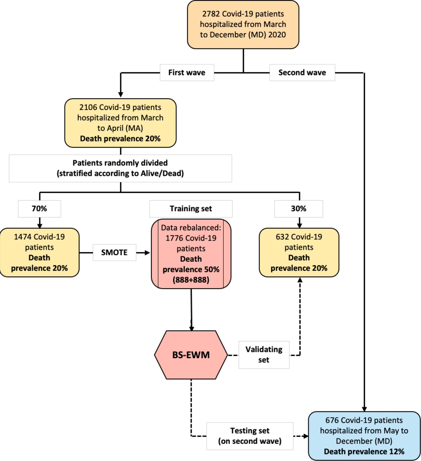
Flowchart of the data used in the empirical analyses.
The early-warning model (BS-EWM) was trained with a random forest on 70% of first-wave patients (rebalanced with the synthetic minority oversampling technique [SMOTE] procedure) and (i) validated on remaining 30% of first-wave patients (ii) tested on 676 second-wave patients. In detail, 2106 patients were randomly in training and validating, maintaining the same death prevalence of the first wave.
Figure 2
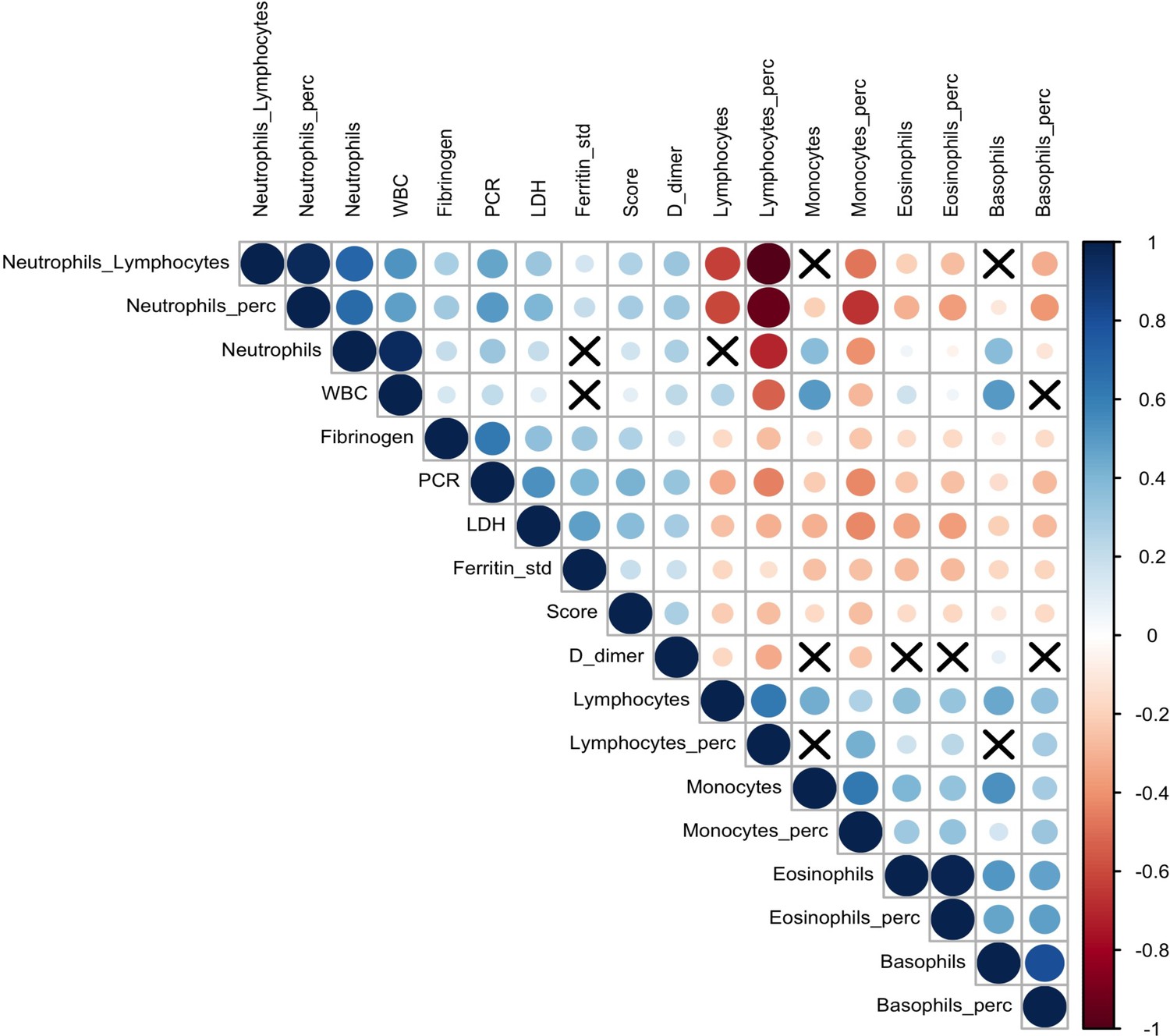
Correlation plot on biomarkers and Brescia chest X-ray score.
The relationships between 17 analytes and Brescia chest X-ray score are inspected with the Spearman correlation coefficients, ρs, which are represented in this correlation plot by means of blue and red circles (positive and negative correlation, respectively). The diameter of the circle is proportional to the magnitude of ρs and black crosses on them identify correlation not significantly different from zero (p-values > 0.05). The correlation matrix is reordered according to the hierarchical cluster analysis on the quantitative variables.
Figure 3
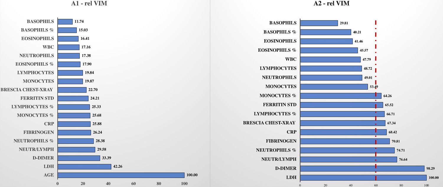
Relative variable importance measure (rel VIM).
In , Figure 3, A1, there is the rel VIM based on Gini index. It was extracted from a random forest where the outcome is dead/alive and covariates are: the 17 biomarkers, Brescia X-ray score, and age. The algorithm grows 10,000 trees where the number of splitting variables at each tree node is √(# covariates in the model). Missing values are imputed with the ‘on-the-fly-imputation’ algorithm. A model with the same features was run (Figure 3, A2) excluding the covariate ‘age’ since it was strongly associated with the risk of death, masking the role of remaining covariates.
Figure 4
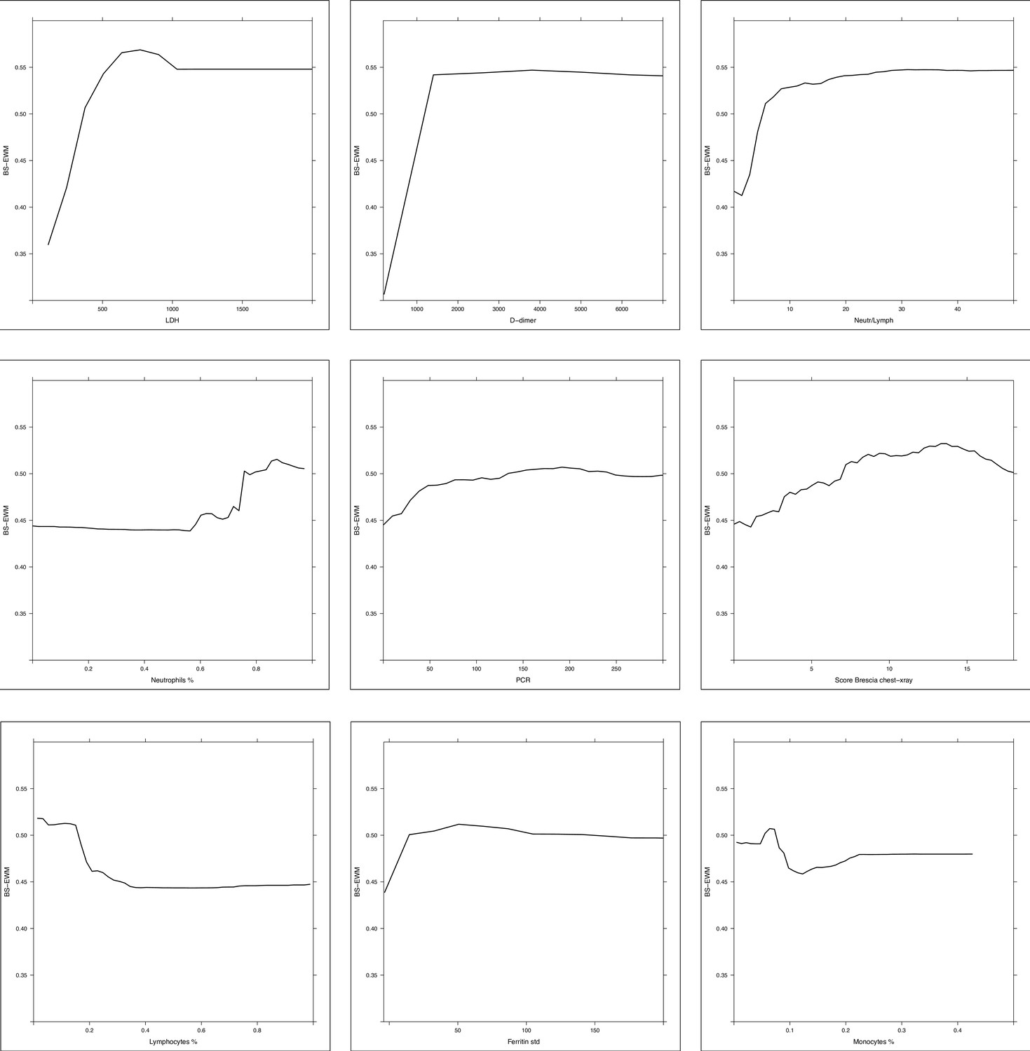
Partial dependence plot (PDP) of random forest grown on the 17 biomarkers and Brescia X-ray score.
Considering the random forest that excludes the ‘age’ variable, the PDPs were computed in correspondence of covariates with relative variable importance measure (rel VIM) of Appendix 1—figure 2 > 60 (cut-off identified by the red dashed line) and p-value in Table 1 < 0.05. Of 10 most important variables in Appendix 1—figure 2, nine satisfy these two conditions (only fibrinogen was excluded since it was not significantly different in the two subpopulations deceased/alive). PDPs measure the effects of changes in covariate values taken one per time, on the risk of death. They are displayed from the most to the less important variable.
Figure 5

Receiver operating characteristic (ROC) curves of random forest, gradient boosting machine (GBM), and logistic regression.
ROC curves of three methods: (i) random forest, (ii) GBM, and (iii) logistic regression. Each graph reports the ROC curve computed in training (blue line, 70% of March–April’s patients), validating (dashed red line, 30% of March–April’s patients), and testing (dashed green lined, May–December’s patients).
Tables
Table 1
Descriptive statistics on all variables in the dataset stratified respect alive–dead. Comparison between first (March–April) and second (May–December) wave.
| Variables | First wave: March–April (MA) 2020 | p-Value | Second wave: May–December (MD) 2020 | p-Value | ||
|---|---|---|---|---|---|---|
| Alive(N = 1683) | Dead(N = 423) | Alive (N = 594) | Dead (N = 82) | |||
| Age | <0.001* | <0.001* | ||||
| Mean (SD) | 64.55 (14.27) | 76.21 (9.12) | 65.30 (15.20) | 76.72 (10.79) | ||
| Median(Q1, Q3) | 65.00(55.00, 75.00) | 77.00(72.00, 82.00) | 67.00(55.00, 77.00) | 80.00(72.25, 84.75) | ||
| Range | 19.00–97.00 | 44.00–98.00 | 18.00–97.00 | 44.00–98.00 | ||
| Sex | 0.036† | 0.131† | ||||
| F | 613 (36.4%) | 131 (31.0%) | 240 (40.4%) | 26 (31.7%) | ||
| M | 1,070 (63.6%) | 292 (69.0%) | 354 (59.6%) | 56 (68.3%) | ||
| Days in hospital | <0.001* | 0.008* | ||||
| N-Miss | 1 | 0 | 95 | 0 | ||
| Mean (SD) | 14.15 (11.66) | 11.33 (10.98) | 14.95 (11.67) | 17.77 (10.75) | ||
| Median(Q1, Q3) | 11.00(7.00, 18.00) | 8.00(4.00, 15.00) | 12.00(7.00, 20.00) | 17.50(9.00, 25.00) | ||
| Range | 0.00–140.00 | 0.00–88.00 | 0.00–79.00 | 2.00–46.00 | ||
| Score | <0.001* | <0.001* | ||||
| Mean (SD) | 6.92 (4.40) | 8.77 (4.39) | 5.65 (4.48) | 8.23 (4.63) | ||
| Median(Q1, Q3) | 7.00(3.00, 10.00) | 9.00(6.00, 12.00) | 5.00(2.00, 9.00) | 9.00(5.25, 11.00) | ||
| Range | 0.00–18.00 | 0.00–18.00 | 0.00–18.00 | 0.00–17.00 | ||
| D-dimer | <0.001* | <0.001* | ||||
| N-Miss | 406 | 113 | 128 | 16 | ||
| Mean (SD) | 1155.03 (2218.51) | 3124.25 (8070.21) | 1538.17 (3123.38) | 4712.44 (8897.82) | ||
| Median(Q1, Q3) | 443.00(262.00, 985.00) | 944.50(476.50, 2970.75) | 739.50(427.50, 1341.25) | 1112.00(725.50, 3619.25) | ||
| Range | 200.00–47228.00 | 200.00–60,342.00 | 190.00–33,501.00 | 190.00–35,000.00 | ||
| Fibrinogen | 0.951* | 0.778* | ||||
| N-Miss | 339 | 117 | 54 | 8 | ||
| Mean (SD) | 530.53 (194.13) | 530.55 (213.69) | 523.94 (169.43) | 519.77 (213.05) | ||
| Median(Q1, Q3) | 520.00(381.00, 650.00) | 515.00(381.00, 654.00) | 512.00(405.00, 612.00) | 510.00(330.50, 649.00) | ||
| Range | 119.00–1339.00 | 68.00–1333.00 | 147.00–1371.00 | 153.00–1287.00 | ||
| LDH | <0.001* | <0.001* | ||||
| N-Miss | 188 | 92 | 61 | 7 | ||
| Mean (SD) | 321.25 (227.50) | 433.71 (205.10) | 308.30 (196.23) | 443.49 (707.95) | ||
| Median(Q1, Q3) | 283.00(222.00, 373.00) | 406.00(269.50, 545.50) | 273.00(218.00, 354.00) | 332.00(257.00, 442.50) | ||
| Range | 90.00–6689.00 | 123.00–1365.00 | 108.00–2565.00 | 122.00–6310.00 | ||
| Neutrophils | <0.001* | <0.001* | ||||
| N-Miss | 23 | 19 | 4 | 1 | ||
| Mean (SD) | 5.67 (3.61) | 7.17 (4.39) | 5.80 (3.97) | 7.21 (4.13) | ||
| Median(Q1, Q3) | 4.83(3.29, 7.03) | 6.20(4.12, 9.02) | 4.78(3.42, 7.11) | 6.72(4.00, 9.77) | ||
| Range | 0.00–53.99 | 0.17–30.45 | 0.10–47.03 | 0.19–23.02 | ||
| Lymphocytes | <0.001* | <0.001* | ||||
| N-Miss | 23 | 19 | 4 | 1 | ||
| Mean (SD) | 1.43 (5.48) | 1.19 (4.29) | 1.22 (0.81) | 1.38 (4.63) | ||
| Median(Q1, Q3) | 1.04(0.75, 1.42) | 0.81(0.55, 1.18) | 1.06(0.72, 1.52) | 0.74(0.47, 1.06) | ||
| Range | 0.10–177.63 | 0.04–85.51 | 0.08–10.28 | 0.08–42.20 | ||
| Neutrophils on lymphocytes | <0.001* | <0.001* | ||||
| N-Miss | 23 | 19 | 4 | 1 | ||
| Mean (SD) | 6.18 (5.87) | 10.72 (11.71) | 7.19 (9.92) | 12.84 (13.09) | ||
| Median(Q1, Q3) | 4.52(2.84, 7.50) | 7.13(4.47, 13.06) | 4.32(2.63, 8.40) | 8.50(4.05, 15.19) | ||
| Range | 0.00–101.90 | 0.01–129.67 | 0.12–143.25 | 0.11–70.56 | ||
| Neutrophils % | <0.001* | <0.001* | ||||
| N-Miss | 22 | 19 | 4 | 1 | ||
| Mean (SD) | 0.73 (0.13) | 0.80 (0.12) | 0.73 (0.13) | 0.79 (0.16) | ||
| Median(Q1, Q3) | 0.74(0.66, 0.82) | 0.82(0.75, 0.88) | 0.73(0.64, 0.83) | 0.83(0.69, 0.89) | ||
| Range | 0.00–0.97 | 0.01–0.97 | 0.10–0.99 | 0.10–0.96 | ||
| Lymphocytes % | <0.001* | <0.001* | ||||
| N-Miss | 22 | 19 | 4 | 1 | ||
| Mean (SD) | 0.18 (0.11) | 0.13 (0.09) | 0.18 (0.11) | 0.13 (0.13) | ||
| Median(Q1, Q3) | 0.16(0.11, 0.23) | 0.11(0.07, 0.17) | 0.17(0.10, 0.25) | 0.10(0.06, 0.18) | ||
| Range | 0.01–0.97 | 0.01–0.99 | 0.01–0.88 | 0.01–0.88 | ||
| PCR | <0.001* | 0.004* | ||||
| N-Miss | 47 | 12 | 21 | 0 | ||
| Mean (SD) | 77.25 (75.76) | 117.68 (95.97) | 64.28 (73.38) | 98.59 (102.49) | ||
| Median(Q1, Q3) | 55.65(17.30, 111.60) | 99.20(42.80, 170.45) | 39.10(12.30, 91.10) | 74.80(20.12, 140.73) | ||
| Range | 0.30–479.00 | 0.70–471.10 | 0.30–483.20 | 0.30–593.80 | ||
| WBC | <0.001* | 0.011* | ||||
| N-Miss | 21 | 19 | 4 | 1 | ||
| Mean (SD) | 7.73 (7.13) | 9.13 (7.46) | 7.65 (4.17) | 9.23 (6.25) | ||
| Median(Q1, Q3) | 6.62(4.87, 9.11) | 7.62(5.60, 10.74) | 6.67(5.02, 8.90) | 8.34(5.55, 12.04) | ||
| Range | 0.72–191.02 | 0.32–92.23 | 0.97–48.19 | 0.97–47.79 | ||
| Basophils | 0.073* | 0.419* | ||||
| N-Miss | 23 | 19 | 4 | 1 | ||
| Mean (SD) | 0.02 (0.02) | 0.02 (0.02) | 0.02 (0.04) | 0.02 (0.02) | ||
| Median(Q1, Q3) | 0.01(0.01, 0.02) | 0.01(0.01, 0.02) | 0.02(0.01, 0.03) | 0.01(0.01, 0.03) | ||
| Range | 0.00–0.31 | 0.00–0.15 | 0.00–0.84 | 0.00–0.11 | ||
| Basophils % | <0.001* | 0.024* | ||||
| N-Miss | 22 | 19 | 4 | 1 | ||
| Mean (SD) | 0.00 (0.00) | 0.00 (0.00) | 0.00 (0.00) | 0.00 (0.00) | ||
| Median(Q1, Q3) | 0.00(0.00, 0.00) | 0.00(0.00, 0.00) | 0.00(0.00, 0.00) | 0.00(0.00, 0.00) | ||
| Range | 0.00–0.02 | 0.00–0.06 | 0.00–0.05 | 0.00–0.01 | ||
| Eosinophils | <0.001* | 0.015* | ||||
| N-Miss | 23 | 19 | 4 | 1 | ||
| Mean (SD) | 0.06 (0.12) | 0.04 (0.10) | 0.06 (0.14) | 0.05 (0.13) | ||
| Median(Q1, Q3) | 0.01 (0.00, 0.07) | 0.00 (0.00, 0.02) | 0.01 (0.00, 0.06) | 0.00 (0.00, 0.03) | ||
| Range | 0.00–2.19 | 0.00–0.79 | 0.00–1.95 | 0.00–0.97 | ||
| Eosinophils % | <0.001* | 0.013* | ||||
| N-Miss | 22 | 19 | 4 | 1 | ||
| Mean (SD) | 0.01 (0.02) | 0.00 (0.01) | 0.01 (0.02) | 0.01 (0.01) | ||
| Median(Q1, Q3) | 0.00(0.00, 0.01) | 0.00(0.00, 0.00) | 0.00(0.00, 0.01) | 0.00(0.00, 0.00) | ||
| Range | 0.00–0.27 | 0.00–0.12 | 0.00–0.25 | 0.00–0.07 | ||
| Monocytes | <0.001* | 0.683* | ||||
| N-Miss | 23 | 19 | 4 | 1 | ||
| Mean (SD) | 0.56 (0.68) | 0.69 (3.32) | 0.55 (0.32) | 0.58 (0.41) | ||
| Median(Q1, Q3) | 0.47(0.32, 0.68) | 0.41(0.25, 0.63) | 0.49(0.33, 0.68) | 0.48(0.27, 0.77) | ||
| Range | 0.01–23.31 | 0.02–66.34 | 0.02–2.45 | 0.07–2.01 | ||
| Monocytes % | <0.001* | 0.034* | ||||
| N-Miss | 22 | 19 | 4 | 1 | ||
| Mean (SD) | 0.08 (0.04) | 0.07 (0.05) | 0.08 (0.04) | 0.07 (0.05) | ||
| Median(Q1, Q3) | 0.07 (0.05, 0.10) | 0.06 (0.04, 0.08) | 0.07 (0.05, 0.10) | 0.06 (0.04, 0.09) | ||
| Range | 0.00–0.70 | 0.01–0.72 | 0.01–0.31 | 0.01–0.27 | p-Value | |
| Ferritin F | 613 patients(82.39%) | 131 patients(17.61%) | <0.001* | 240 patients(90.23%) | 26 patients(9.77%) | 0.372* |
| N-Miss | 158 | 34 | 43 | 5 | ||
| Mean (SD) | 674.53 (817.61) | 1237.07 (2308.64) | 564.63 (526.39) | 2006.00 (4680.23) | ||
| Median(Q1, Q3) | 459.00(212.00, 820.50) | 700.00(353.00, 1347.00) | 433.00(216.00, 750.00) | 510.00(269.00, 722.00) | ||
| Range | 4.00–7687.00 | 19.00–20,572.00 | 11.00–3397.00 | 81.00–20,941.00 | ||
| Ferritin M | 1070 patients(78.56%) | 292 patients(21.44%) | <0.001* | 354 patients(90.23%) | 56 patients(9.77%) | 0.007* |
| N-Miss | 257 | 96 | 50 | 5 | ||
| Mean (SD) | 1353.00 (1359.86) | 1825.25 (1945.47) | 1181.95 (3295.92) | 1372.04 (1258.14) | ||
| Median(Q1, Q3) | 939.00(461.00, 1705.00) | 1262.50(572.25, 2323.25) | 737.50(405.25, 1283.00) | 1159.00(598.00, 1500.00) | ||
| Range | 23.00–11,513.00 | 55.00–13,289.00 | 25.00–56,039.00 | 112.00–7058.00 | ||
-
In bold and italics p-values < 0.05.
-
*
Wilcoxon rank-sum test.
-
†
Fisher’s exact test.
Table 2
Performance metrics of methods: random forest, gradient boosting machine (GBM), and logistic regression.
| Metrics | Random forest | GBM | Logistic regression | ||||||
|---|---|---|---|---|---|---|---|---|---|
| TrainingMarch–April (MA) | ValidatingMarch–April (MA) | TestingMay–Dec(MD) | TrainingMarch–April (MA) | ValidatingMarch–April (MA) | TestingMay–Dec(MD) | TrainingMarch–April (MA) | ValidatingMarch–April (MA) | TestingMay–Dec(MD) | |
| AUC (DeLong)(95% CI) | 0.97(0.97–0.98) | 0.83(0.80–0.87) | 0.78(0.73–0.84) | 0.88(0.86–0.89) | 0.84(0.80–0.88) | 0.78(0.73–0.83) | 0.84(0.82–0.86) | 0.83(0.79–0.87) | 0.52(0.44–0.60) |
| Sensitivity(95% CI) | 0.93(0.91–0.97) | 0.82(0.72–0.92) | 0.73(0.54–1.00) | 0.85(0.80–0.88) | 0.80(0.66–0.90) | 0.77(0.65–0.94) | 0.80(0.77–0.84) | 0.84(0.76–0.91) | 0.87(0.18–1.00) |
| Specificity(95% CI) | 0.92(0.88–0.94) | 0.75(0.63–0.83) | 0.73(0.41–0.89) | 0.77(0.73–0.81) | 0.75(0.65–0.87) | 0.71(0.50–0.79) | 0.74(0.70–0.77) | 0.73(0.65–0.79) | 0.26(0.11–0.94) |
-
Comparison between the performances of three methods: random forest, GBM, and logistic regression model applied on the rebalanced dataset obtained with SMOTE methodology. Logistic regression predictions are computed using the 10-fold cross-validation in order to be comparable with random forest and GBM predictions (which use out-of-bag and 10-fold cross-validation, respectively).
Additional files
-
Supplementary file 1
Descriptive statistics on all variables.
(a) Descriptive statistics on all variables of the entire sample.
(b) Descriptive statistics on all variables in the dataset stratified respect first (March–April 2020) and second (May–December 2020) wave. Comparison between alive and dead. (c): Performance metrics of the random forest (RF) using or not a rebalanced dataset with the synthetic minority oversampling technique (SMOTE) methodology. In this table we compare the performance of two RFs applied on (i) a dataset rebalanced with the SMOTE methodology and (ii) the original dataset. This analysis suggests the use of SMOTE methodology before applying RF since the performance in training and validating groups (especially in terms of sensitivity) are better respect those obtained from the RF grown on the original dataset. (d): Performance metrics of the random forests (RFs) estimated on single biomarkers. (e): Optimal threshold for each biomarker to predict the outcome.
- https://cdn.elifesciences.org/articles/70640/elife-70640-supp1-v3.docx
Download links
A two-part list of links to download the article, or parts of the article, in various formats.
Downloads (link to download the article as PDF)
Open citations (links to open the citations from this article in various online reference manager services)
Cite this article (links to download the citations from this article in formats compatible with various reference manager tools)
Early prediction of in-hospital death of COVID-19 patients: a machine-learning model based on age, blood analyses, and chest x-ray score
eLife 10:e70640.
https://doi.org/10.7554/eLife.70640


